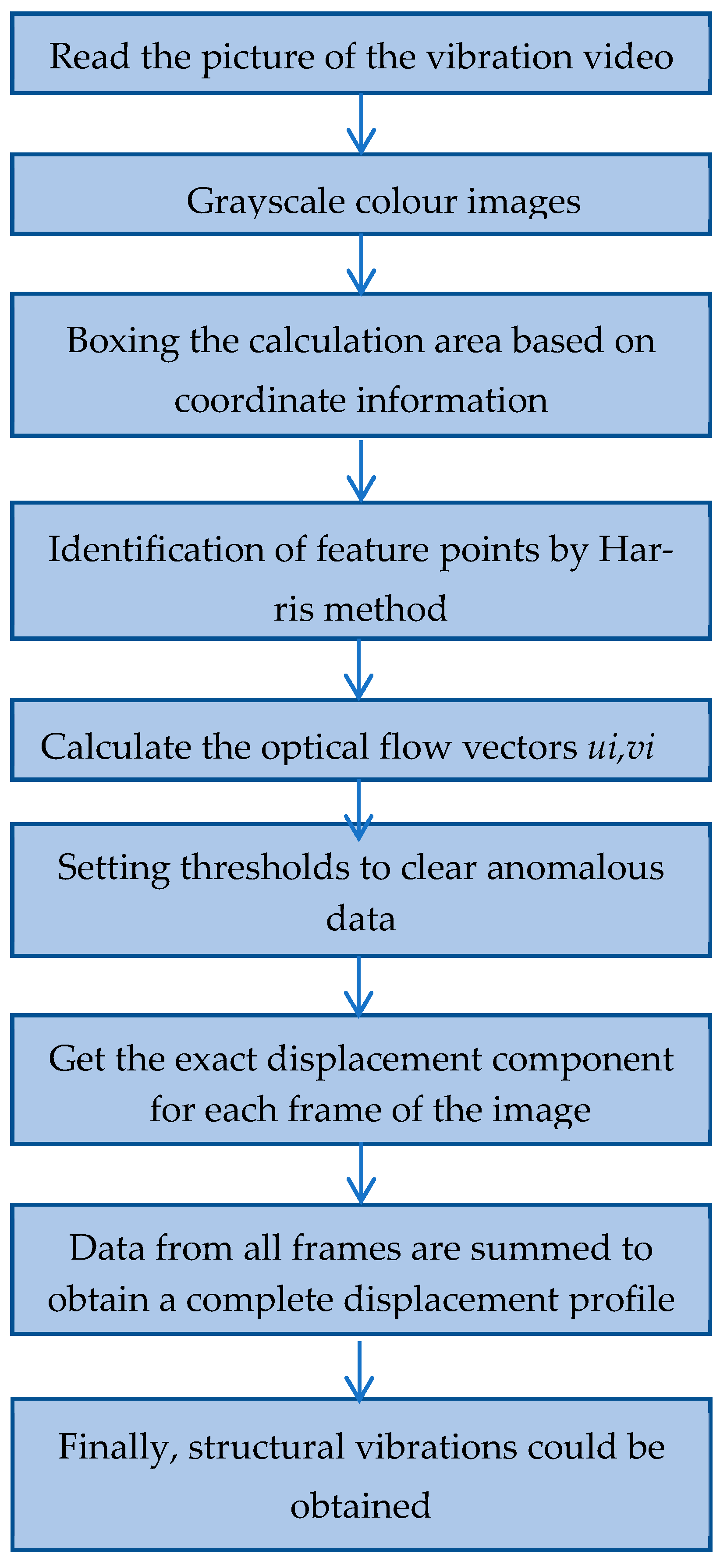
Figure 1.
Flowchart of the Enhanced Optical Flow Method for Precise Vibration Data Acquisition.
Figure 1.
Flowchart of the Enhanced Optical Flow Method for Precise Vibration Data Acquisition.
Figure 2.
Image Projections in Diverse Planes upon Camera Inversion, the blue dots are for four stationary reference points on the original image plane, the red dots are for four stationary reference points on other frames.
Figure 2.
Image Projections in Diverse Planes upon Camera Inversion, the blue dots are for four stationary reference points on the original image plane, the red dots are for four stationary reference points on other frames.
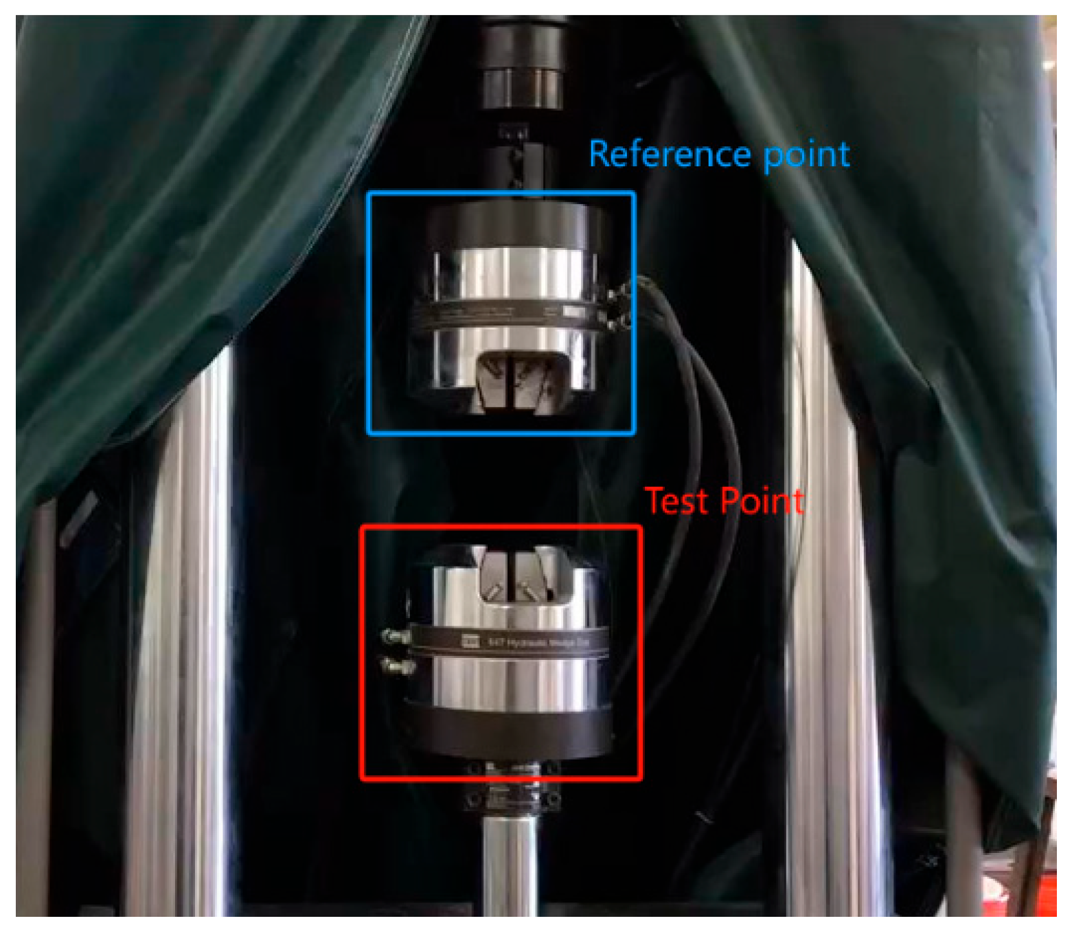
Figure 3.
Selection of a Stationary Reference Point to Mitigate and Eliminate Camera Shake Effects.
Figure 3.
Selection of a Stationary Reference Point to Mitigate and Eliminate Camera Shake Effects.
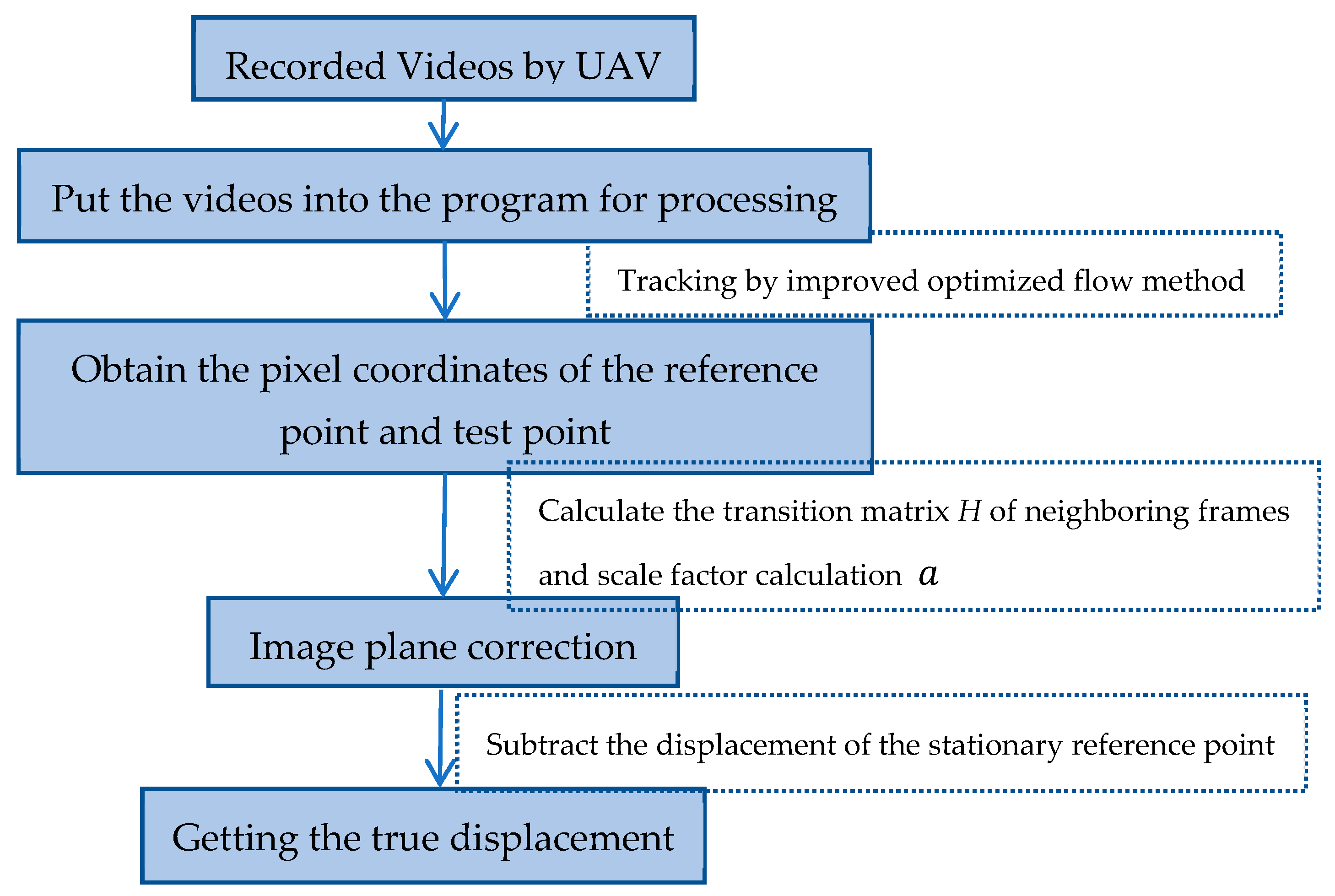
Figure 4.
The computational process of obtaining the real displacement from the drone video.
Figure 4.
The computational process of obtaining the real displacement from the drone video.
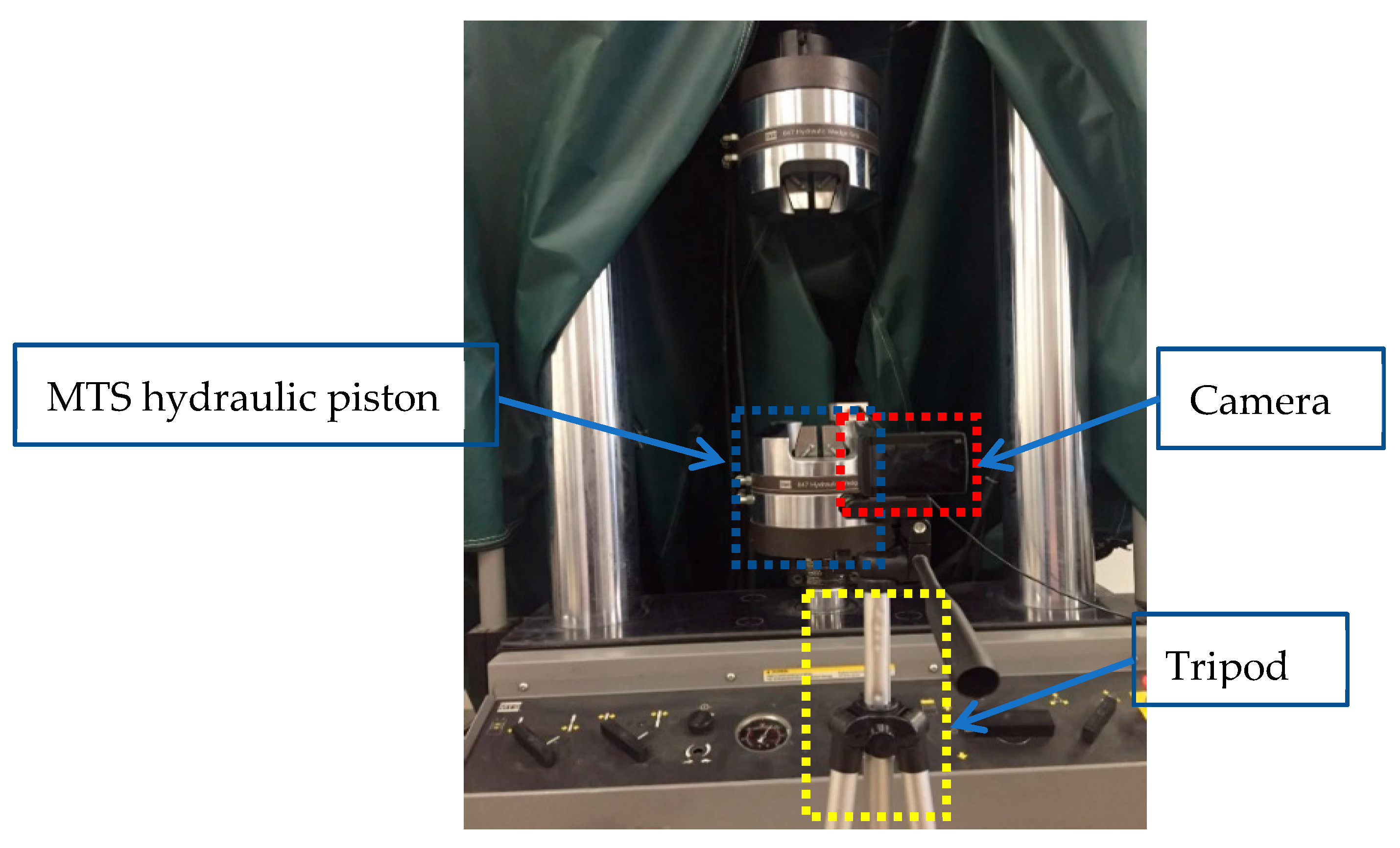
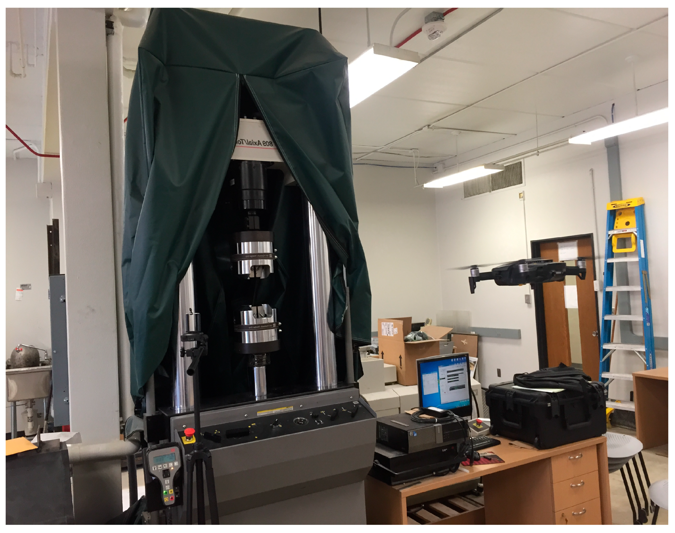
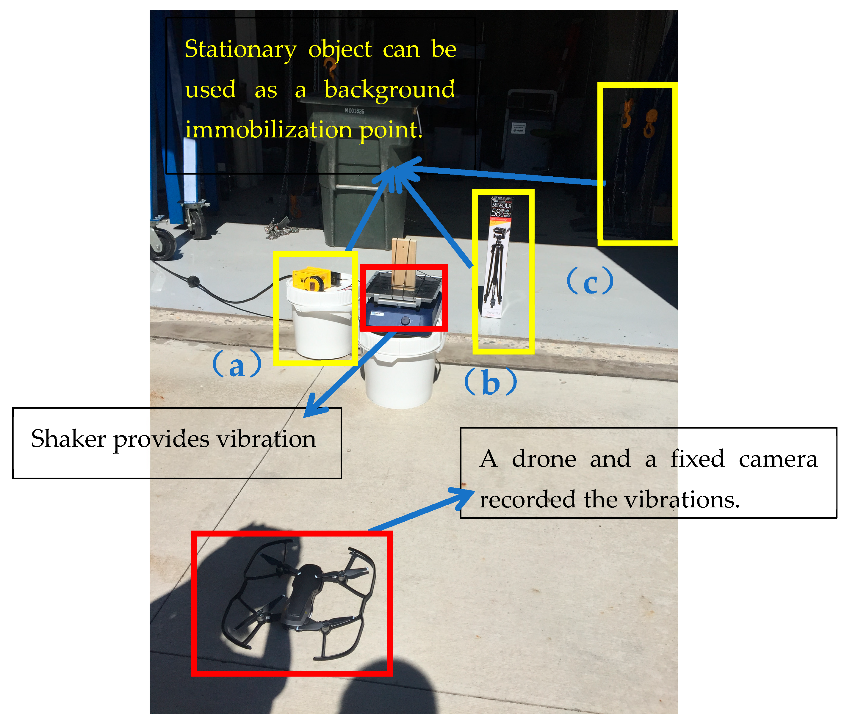
Figure 5.
Layout of the experimental equipment.
Figure 5.
Layout of the experimental equipment.
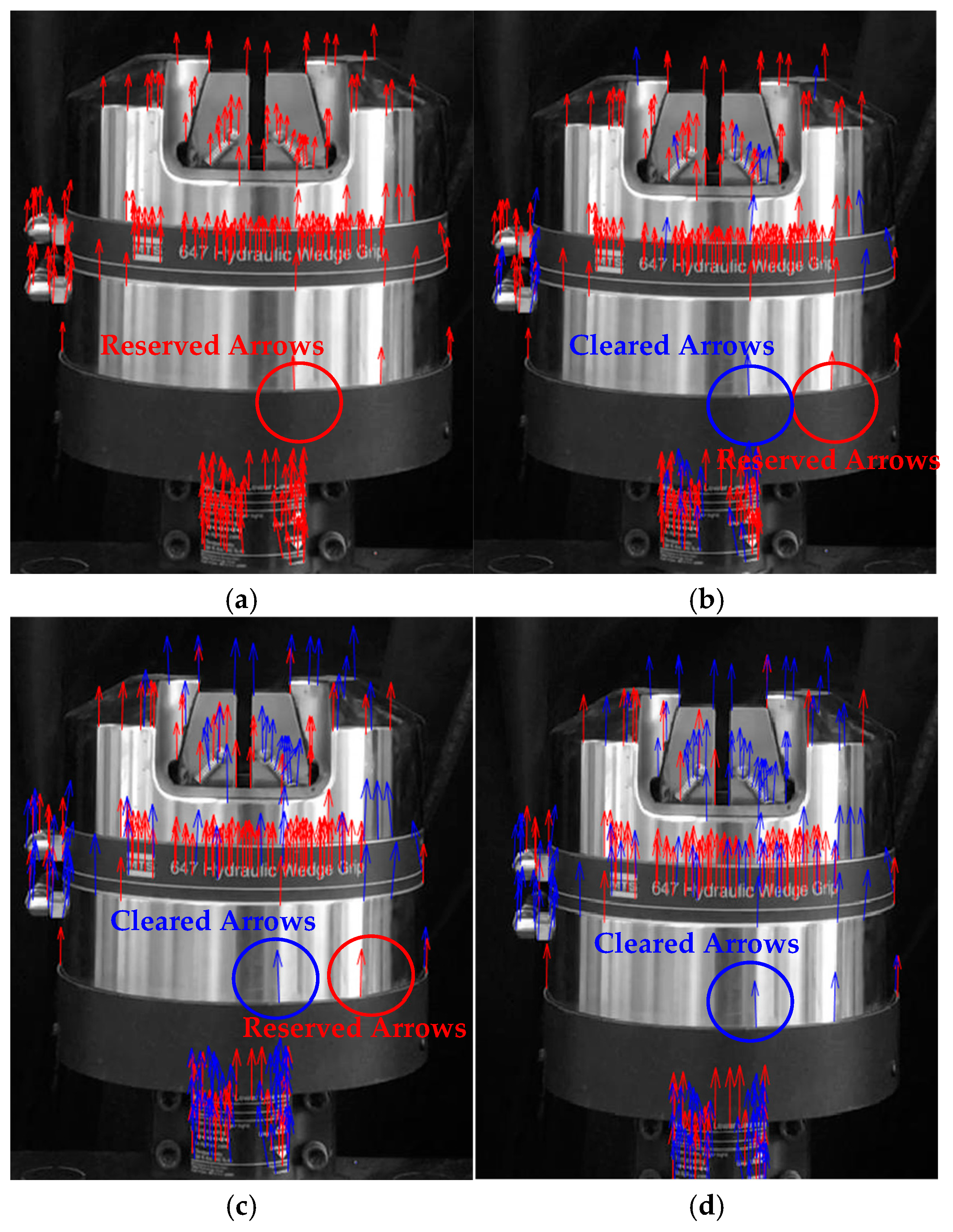
Figure 6.
The motion trajectories of the detected feature points are represented by arrows. Red arrows signify that the coordinate points at the starting ends of these arrows are the retained feature points, while blue arrows indicate that the coordinate points at the starting ends of their arrows are the eliminated feature points. (a) Shows all the detected feature points along with their corresponding arrows. (b) Displays all the detected feature points whose angles are smaller than the threshold of 1×σ, together with their arrows. (c) Presents all the detected feature point arrows for which the angles are less than the threshold value of 0.5×σ. (d) Illustrates all the detected feature point arrows with angles smaller than the threshold value of 0.3×σ.
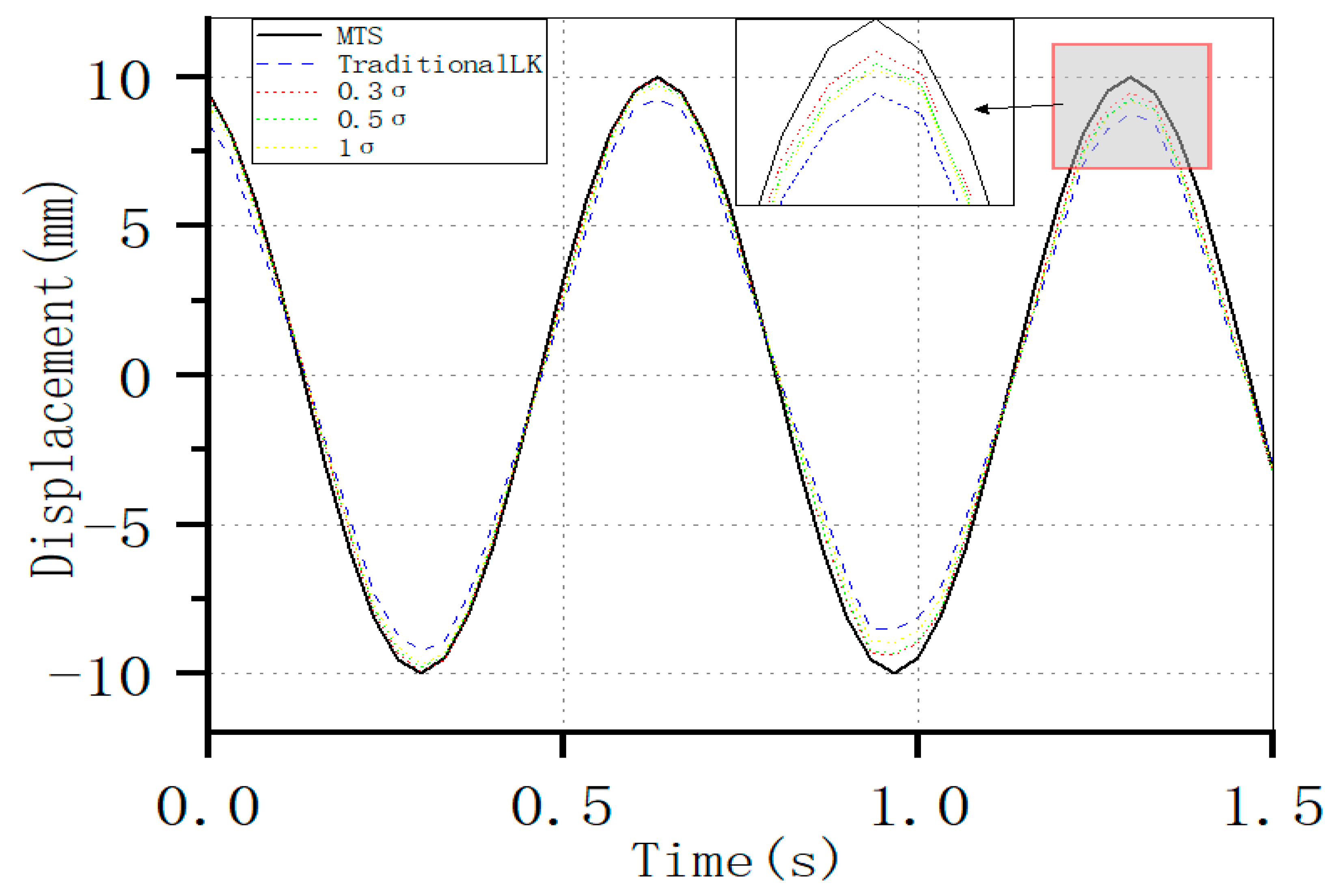
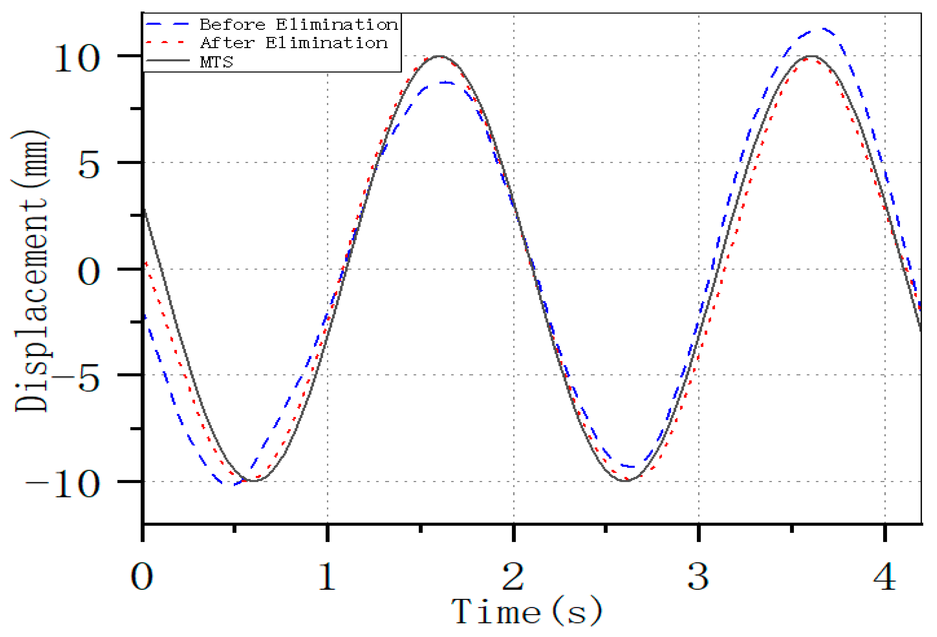
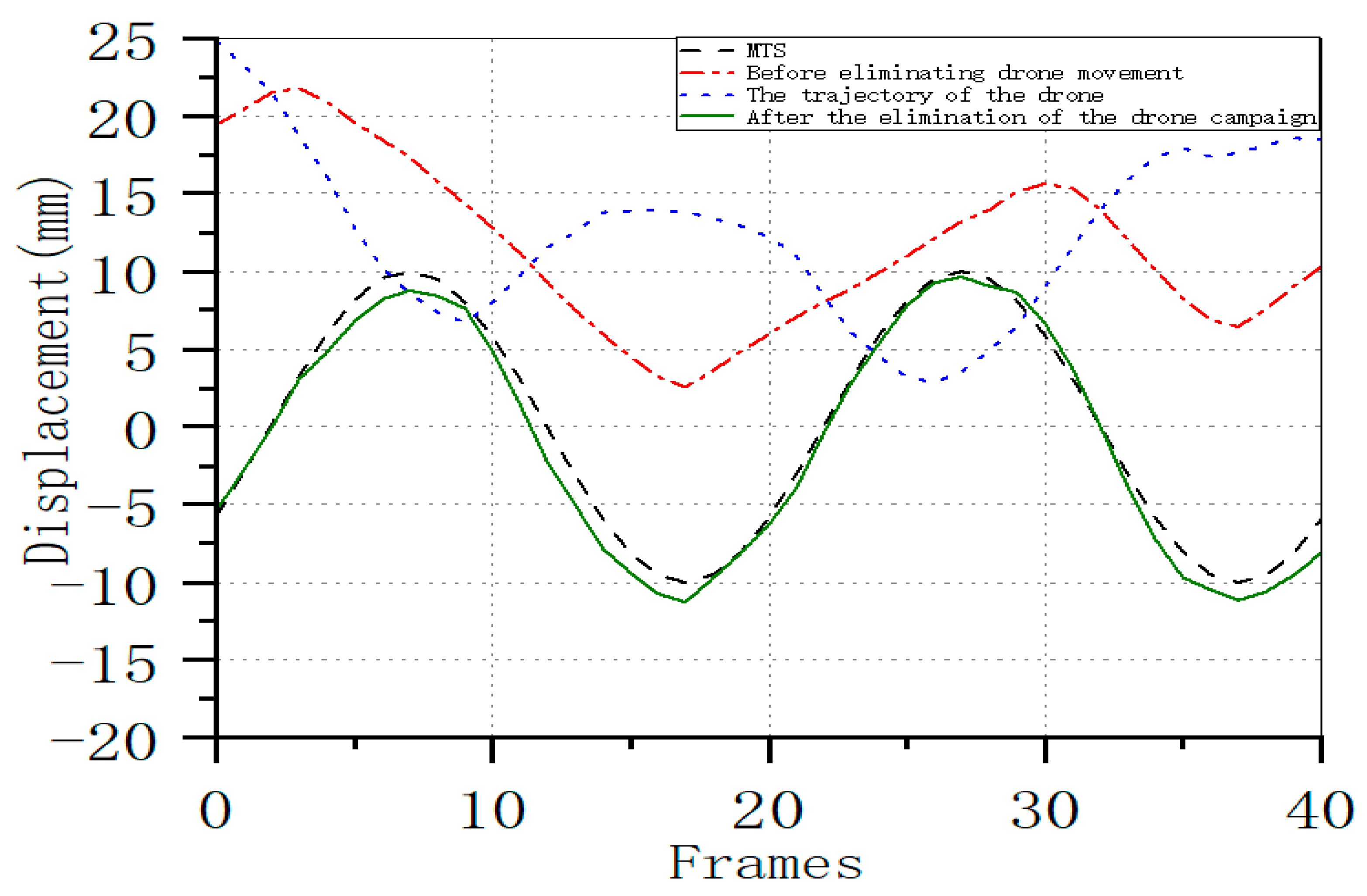
Figure 7.
Comparison between the Data Calculated by the Optical Flow Method Before and After Improvement and the Curve of the MTS Output (at 0.5 Hz).
Figure 7.
Comparison between the Data Calculated by the Optical Flow Method Before and After Improvement and the Curve of the MTS Output (at 0.5 Hz).
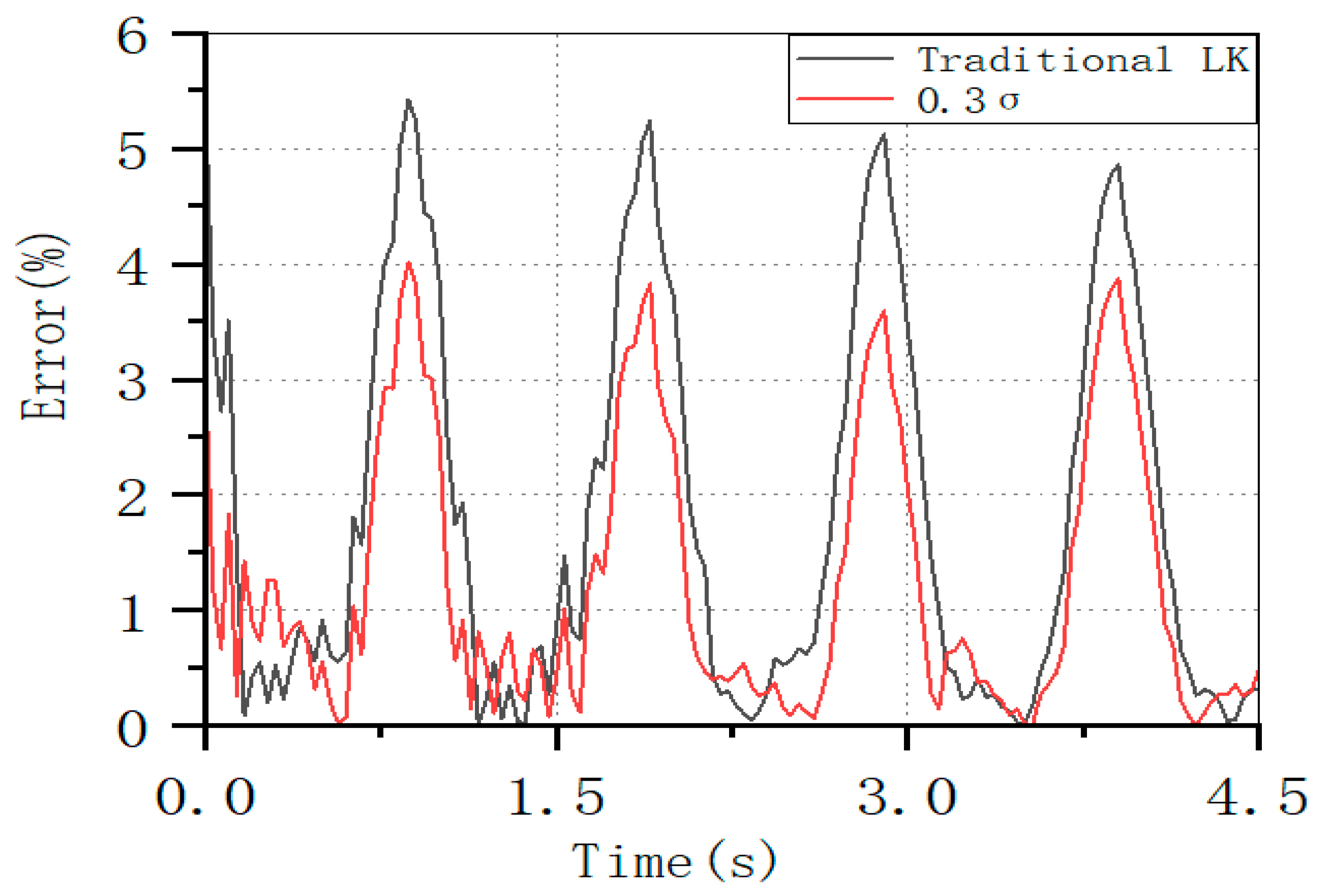
Figure 8.
Comparison of Data Errors Calculated by the Optical Flow Method at Each Temporal Moment: Before and After the Improvement (at 0.5 Hz).
Figure 8.
Comparison of Data Errors Calculated by the Optical Flow Method at Each Temporal Moment: Before and After the Improvement (at 0.5 Hz).
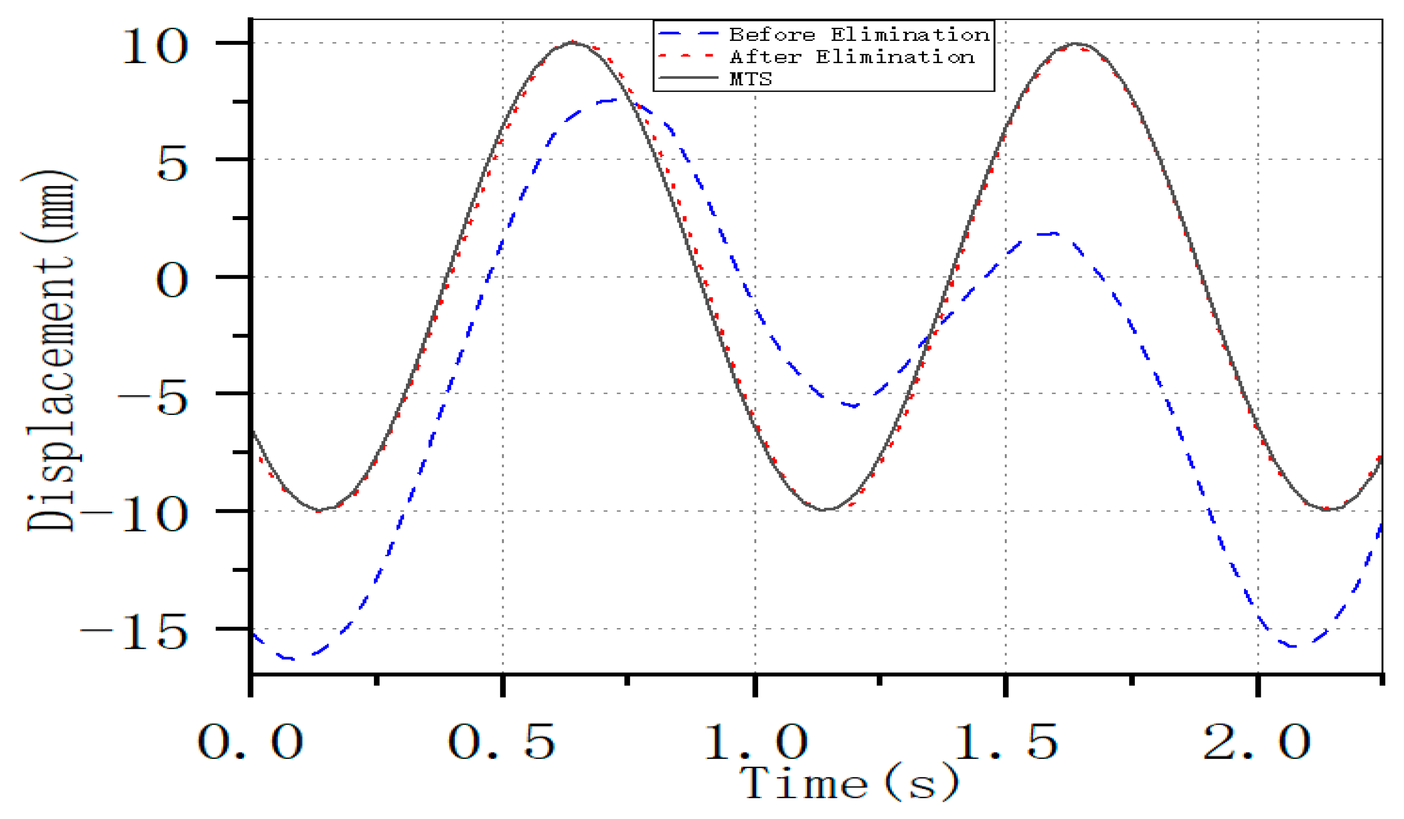
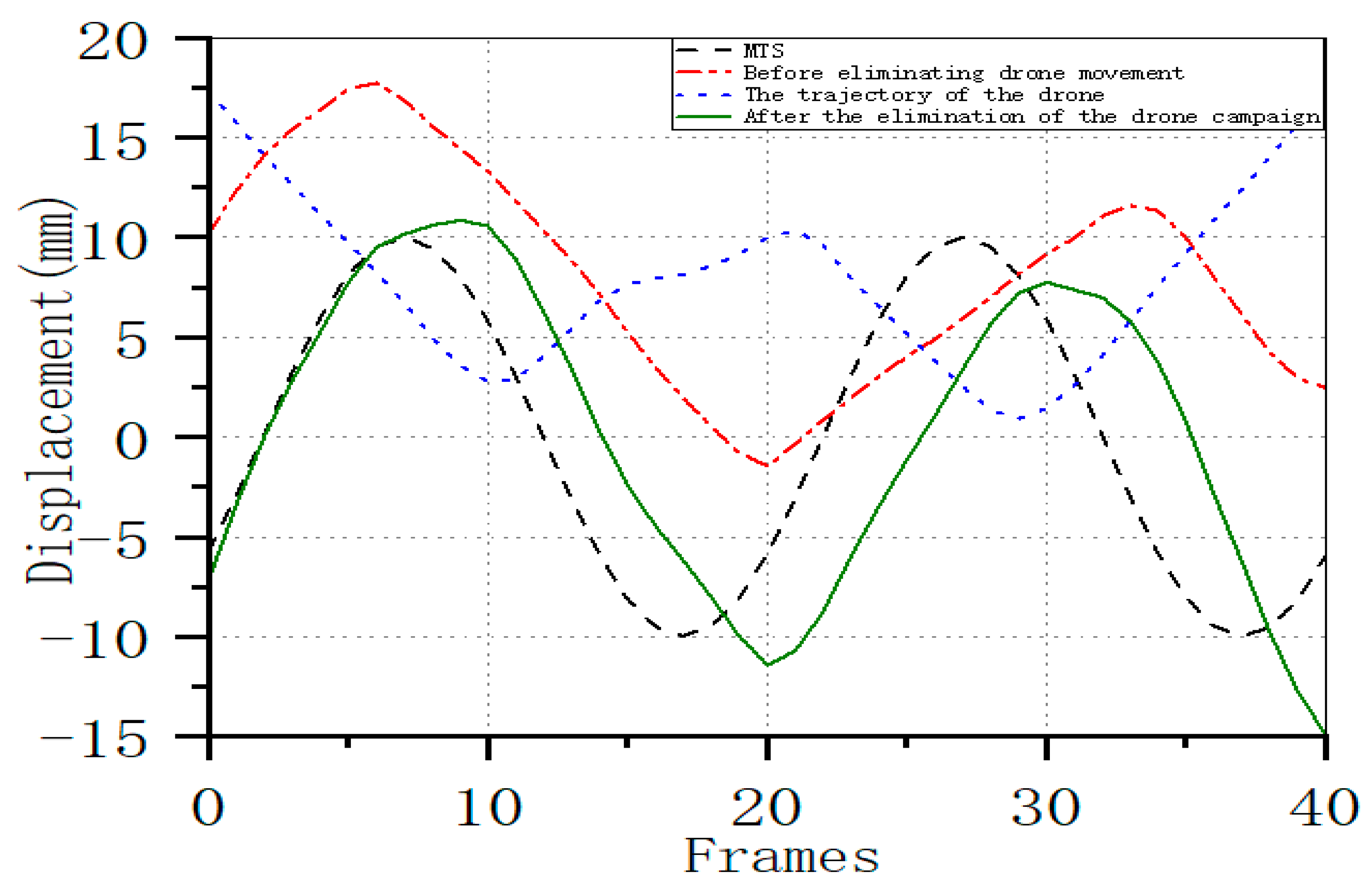
Figure 9.
Comparison between the Data Calculated by the Optical Flow Method Before and After Improvement and the Curves Output by MTS (at 1.5 Hz).
Figure 9.
Comparison between the Data Calculated by the Optical Flow Method Before and After Improvement and the Curves Output by MTS (at 1.5 Hz).
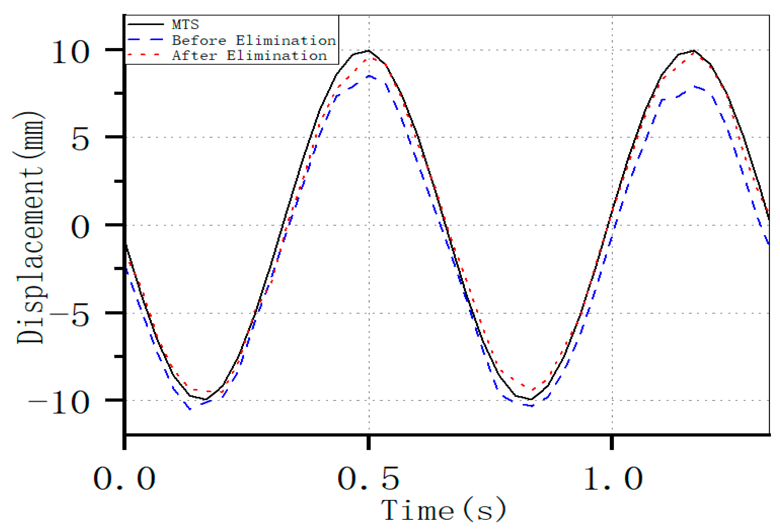
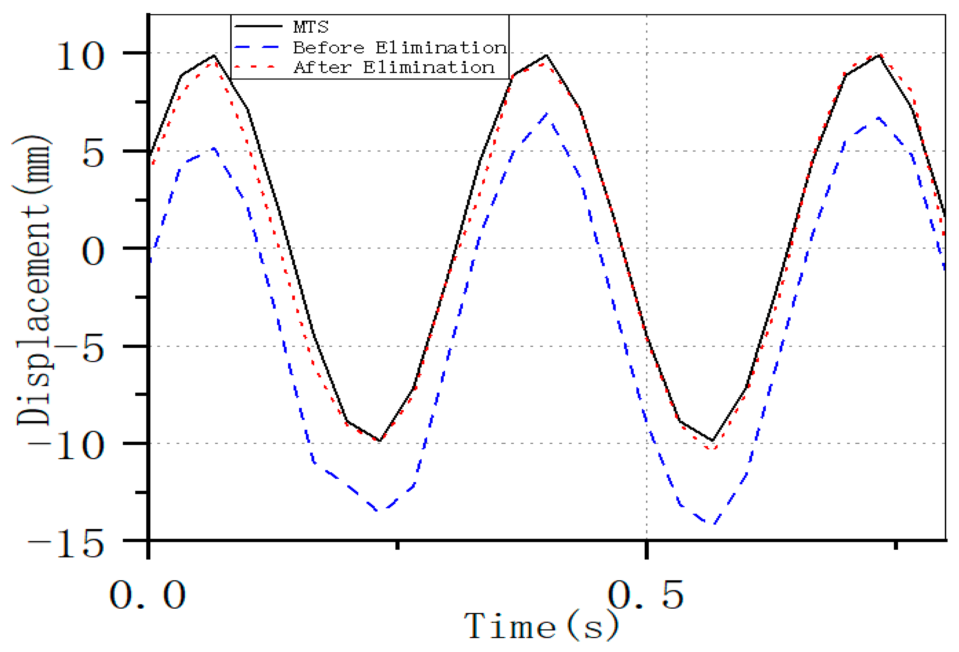
Figure 10.
Comparison of Displacement Curves Before and After Elimination with MTS Output Curves (at 1.5 Hz).
Figure 10.
Comparison of Displacement Curves Before and After Elimination with MTS Output Curves (at 1.5 Hz).
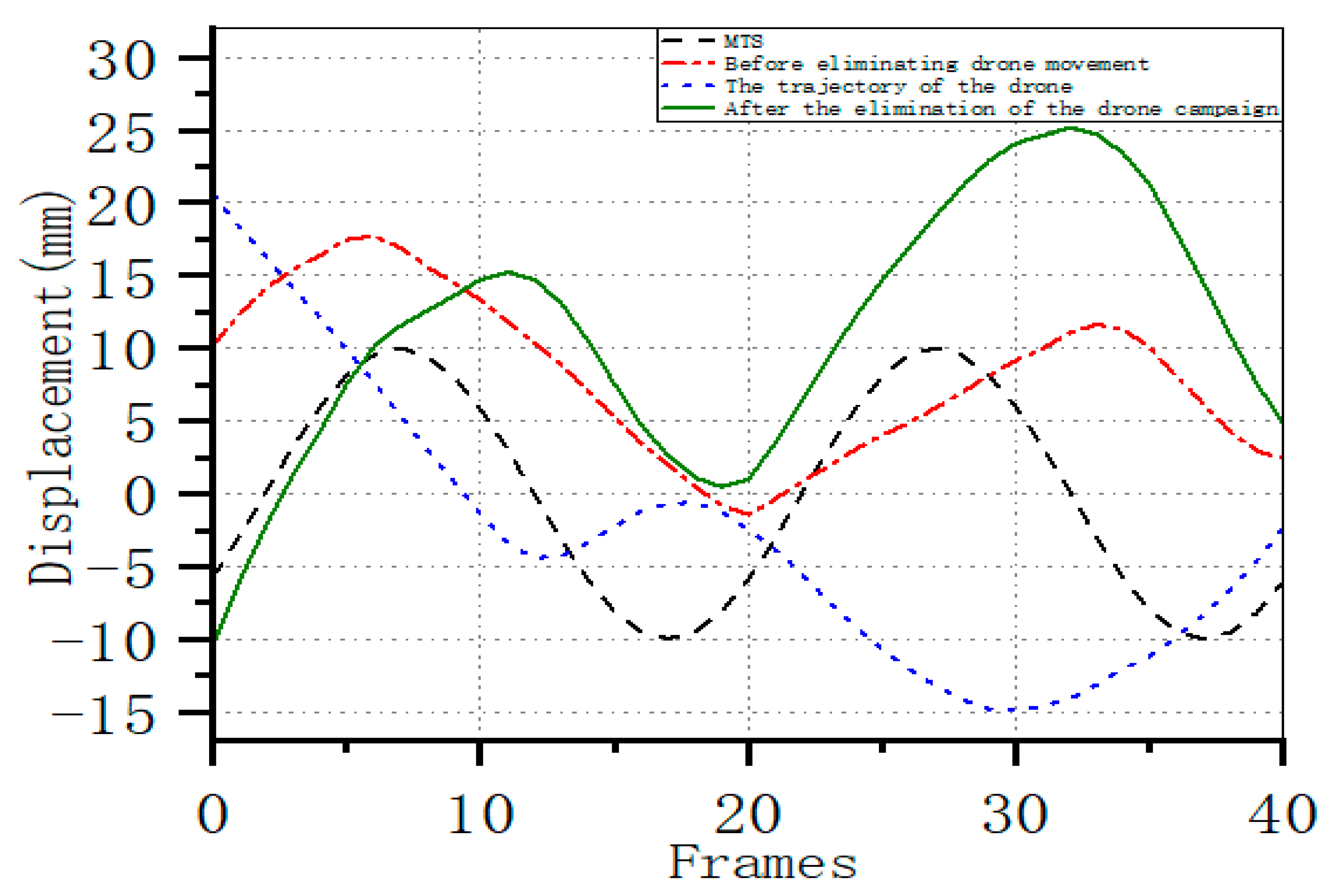
Figure 11.
Comparison of Displacement Curves Before and After Elimination with MTS Output Curves (at 3 Hz).
Figure 11.
Comparison of Displacement Curves Before and After Elimination with MTS Output Curves (at 3 Hz).
Figure 12.
Set up of the UAV experiment.
Figure 12.
Set up of the UAV experiment.
Figure 13.
Equipment for the experiment.
Figure 13.
Equipment for the experiment.
Figure 14.
Comparison of Displacement Curves Before and After Drone Noise Cancellation with MTS Output Curves (at 0.5 Hz).
Figure 14.
Comparison of Displacement Curves Before and After Drone Noise Cancellation with MTS Output Curves (at 0.5 Hz).
Figure 15.
Comparison of Displacement Curves Before and After Drone Noise Cancellation with MTS Output Curves (at 1 Hz).
Figure 15.
Comparison of Displacement Curves Before and After Drone Noise Cancellation with MTS Output Curves (at 1 Hz).
Figure 16.
Equipment layout of UAV experiment outside lab (a) Tool Bucket; (b) Cardboard Box; (c) Iron Mesh.
Figure 16.
Equipment layout of UAV experiment outside lab (a) Tool Bucket; (b) Cardboard Box; (c) Iron Mesh.
Figure 17.
Separate identification of characteristic corner points of selected stationary objects by the program.
Figure 17.
Separate identification of characteristic corner points of selected stationary objects by the program.
Figure 18.
Comparison of the Displacement Curve After UAV Trajectory Elimination with the MTS Output Curve, Taking the Tool Bucket (a) as the Reference (at 3 Hz).
Figure 18.
Comparison of the Displacement Curve After UAV Trajectory Elimination with the MTS Output Curve, Taking the Tool Bucket (a) as the Reference (at 3 Hz).
Figure 19.
Displacement Curve After Eliminating UAV Trajectory Compared with the MTS Output Curve, Using the Cardboard Box (b) as the Reference (at 3 Hz).
Figure 19.
Displacement Curve After Eliminating UAV Trajectory Compared with the MTS Output Curve, Using the Cardboard Box (b) as the Reference (at 3 Hz).
Figure 20.
Displacement Curve After Eliminating UAV Trajectory Compared with the MTS Output Curve, Taking the Iron Mesh (c) as the Reference (at 3 Hz).
Figure 20.
Displacement Curve After Eliminating UAV Trajectory Compared with the MTS Output Curve, Taking the Iron Mesh (c) as the Reference (at 3 Hz).
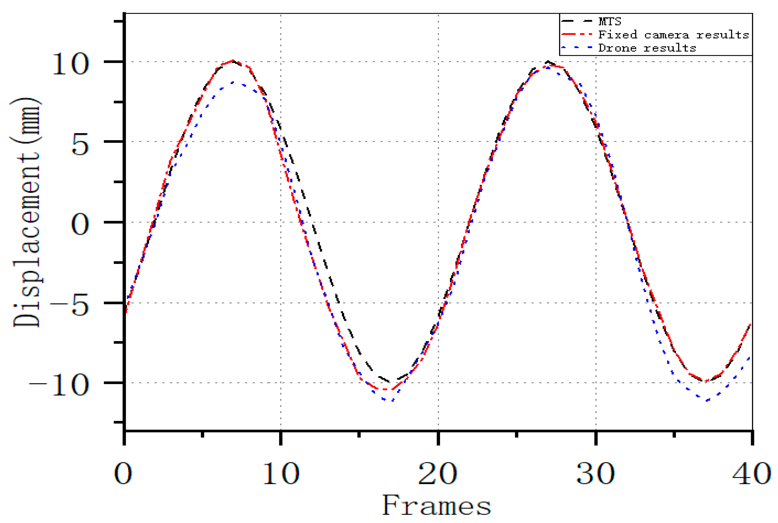
Figure 21.
Comparison of the Displacement Curves Computed by the Improved LK Method with the MTS Output Curves, Where the Displacement Curves are Derived from Data Collected by Fixed Cameras and UAV Cameras.
Figure 21.
Comparison of the Displacement Curves Computed by the Improved LK Method with the MTS Output Curves, Where the Displacement Curves are Derived from Data Collected by Fixed Cameras and UAV Cameras.
Table 1.
Quantities of Retained and Removed Feature Corners Under Different Threshold Values.
Table 1.
Quantities of Retained and Removed Feature Corners Under Different Threshold Values.
| Thresholds | 1×σ | 0.5×σ | 0.3×σ |
|---|
| reservations | 186 | 130 | 97 |
| removals | 37 | 93 | 126 |
Table 2.
Accuracy Comparison of Region of Interest Computation: Traditional LK Method vs. Improved LK Method with a Threshold of 0.3×σ (at 0.5 Hz).
Table 2.
Accuracy Comparison of Region of Interest Computation: Traditional LK Method vs. Improved LK Method with a Threshold of 0.3×σ (at 0.5 Hz).
| ROI | Max Pt Region1 | Min Pt Region1 | Max Pt Region2 | Min Pt Region2 |
|---|
| Traditional LK | 95.7% | 95.9% | 95.9% | 96.05% |
| Improved LK | 97.0% | 97.1% | 97.3% | 96.9% |
Table 3.
Accuracy Comparison of Region of Interest Computation: Traditional LK Method versus Improved LK Method with a Threshold of 0.3×σ (at 1.5 Hz).
Table 3.
Accuracy Comparison of Region of Interest Computation: Traditional LK Method versus Improved LK Method with a Threshold of 0.3×σ (at 1.5 Hz).
| ROI | Max Pt Region1 | Min Pt Region1 | Max Pt Region2 | Min Pt Region2 |
|---|
| Traditional LK | 91.4% | 90.0% | 86.2% | 87.3% |
| Improved LK | 98.6% | 99.3% | 94.4% | 95.9% |
Table 4.
Comparison of accuracy of region of interest computation (1.5 Hz) after eliminating camera vibration with the improved LK method with a threshold of 0.3×σ.
Table 4.
Comparison of accuracy of region of interest computation (1.5 Hz) after eliminating camera vibration with the improved LK method with a threshold of 0.3×σ.
| ROI | Min Pt Region1 | Max Pt Region1 | Min Pt Region2 | Max Pt Region2 |
|---|
| Before elimination | 94.8% | 85.5% | 95.3% | 79.9% |
| After elimination | 96.7% | 95.4% | 96.9% | 96.7% |
Table 5.
Comparison of accuracy of region of interest computation (3 Hz) after eliminating camera vibration with the improved LK method with a threshold of 0.3×σ.
Table 5.
Comparison of accuracy of region of interest computation (3 Hz) after eliminating camera vibration with the improved LK method with a threshold of 0.3×σ.
| ROI | Min Pt Region1 | Max Pt Region1 | Min Pt Region2 | Max Pt Region2 |
|---|
| Before elimination | 59.7% | 65.2% | 56.1% | 70.4% |
| After elimination | 97.7% | 98.6% | 96.2% | 95.7% |
Table 6.
Accuracy Comparison of Region of Interest Calculation for Improved LK Method After UAV Wobble Elimination (0.5 Hz).
Table 6.
Accuracy Comparison of Region of Interest Calculation for Improved LK Method After UAV Wobble Elimination (0.5 Hz).
| ROI | Min Pt Region1 | Max Pt Region1 | Min Pt Region2 | Max Pt Region2 |
|---|
| Before elimination | 90.4% | 88.3% | 93.3% | 87.5% |
| After elimination | 97.9% | 99.1% | 98.0% | 97.9% |
Table 7.
Comparison of the accuracy of the region of interest calculation (1 Hz) for the improved LK method after eliminating UAV wobble.
Table 7.
Comparison of the accuracy of the region of interest calculation (1 Hz) for the improved LK method after eliminating UAV wobble.
| ROI | Min Pt Region1 | Max Pt Region1 | Min Pt Region2 | Max Pt Region2 |
|---|
| Before elimination | 36.6% | 70.2% | 53.9% | 16.6% |
| After elimination | 98.5% | 97.8% | 98.3% | 98.5% |
Table 8.
Precision of calculation results output from the improved LK method (3 Hz) after elimination of UAV trajectories when different reference points are set up.
Table 8.
Precision of calculation results output from the improved LK method (3 Hz) after elimination of UAV trajectories when different reference points are set up.
| Stationary Object | Tool Bucket (a) | Cardboard Box (b) | Iron Mesh (c) |
|---|
| After elimination | 95.5% | 79.7% | 52.7% |
Table 9.
Accuracy Comparison of Region of Interest Calculation for Displacement Curves Derived from the Improved LK Method Based on Fixed and UAV Camera Data.
Table 9.
Accuracy Comparison of Region of Interest Calculation for Displacement Curves Derived from the Improved LK Method Based on Fixed and UAV Camera Data.
| ROI | Max Pt Region1 | Min Pt Region1 | Max Pt Region2 | Min Pt Region2 |
|---|
| Fixed Camera | 97.4% | 94.5% | 98.4% | 98.9% |
| UAV Camera | 92.4% | 92.8% | 96.1% | 90.4% |


