1. Introduction
With the continuous development and improvement of transportation infrastructure in China, the safety monitoring and early warning of bridges in the operation phase have attracted more and more attention [
1,
2]. The performance of bridges, especially large-span cable-stayed bridges, has become a critical area of concern; these structures are subjected to various environmental and operational factors that can significantly impact their structural integrity and longevity [
3]. Along with the bridge quality assessment, bridge structural diseases, how to ensure the safe operation of bridges, and other issues, many major bridge structures have had a structural health monitoring (SHM) system established in order to obtain real-time data on the state of the bridge, assess the performance of the bridge, and provide data and technical basis [
4,
5]. The SHM of long-span cable-stayed bridges is crucial for ensuring their safety and longevity. However, there are still a large number of bridges with low efficiency regarding real-time data processing and providing timely early warnings due to a small monitoring scale, capital investment, and other problems. Therefore, the detection and monitoring of bridge performance, providing a scientific and reasonable assessment and maintenance decision-making, has become a current research hotspot around the world.
The main girder is a very important part of the bridge, and its performance is always a concern. The performance of the main girder will be affected by the environment, load, and other impacts that make the bridge’s structural material performance degrade and decline [
6]. Failure to detect this in time may shorten the service life of the bridge and increase the cost of bridge maintenance as its performance deteriorates, and in severe cases, may lead to sudden ruptures and serious traffic accidents. Large-span cable-stayed bridges are more vulnerable to corrosion and fatigue damage as they are subjected to higher tensile forces during long-term use. The vertical deflection of the main bridge girder is a pivotal indicator of its structural health and is one of the most important items of structural safety and applicability in SHM [
7]. Vertical deflection refers to the linear displacement of the bridge deck axis in the direction perpendicular to the deck, which is caused by factors such as non-uniform temperature changes, automobile loads, and other external forces. The accurate prediction of midspan deflection can help in the early detection of potential structural issues, thereby preventing catastrophic failures [
8]. However, predicting midspan deflection is challenging due to the complex interplay of various factors, such as ambient temperature, vehicle load, and material properties.
Long-span cable-stayed bridges are particularly susceptible to deflections due to their complex structural configuration and the significant forces involved. Deflection monitoring is, thus, a crucial aspect of bridge maintenance and safety assessment [
9]. It allows for the early detection of potential issues, enabling timely interventions to prevent more severe structural damage. Previous research has focused on various methods for deflection assessment and prediction. Studies have utilized techniques such as the additional mass block mass normalization method, modal flexibility method, impact test data analysis, and finite element modeling to predict and analyze bridge deflection. Qi et al. investigated the accuracy and engineering feasibility of the mass normalization method based on additional mass blocks and the modal flexibility method for predicting the modal deflection of bridges with the span of hollow plate girders as the research object [
10]. Tian et al. performed flexibility identification and deflection prediction on a three-span concrete box girder bridge based on impact test data with the predicted deflections in good agreement with the calculated deflections, and the experimental results verified the effectiveness of the method [
11]. Tian et al. proposed a deflection prediction method for post-tensioned concrete continuous box girder bridges based on ambient vibration tests and performed field tests on a three-span bridge to verify the performance and reliability of the proposed method [
12]. While these methods have provided valuable insights, there is still room for improvement in terms of the accuracy of prediction and efficiency. Traditional methods for deflection prediction often rely on empirical models or finite element analysis, which may not fully capture the dynamic and nonlinear behavior of the bridge under varying load conditions. Accurately predicting and understanding bridge deflection is challenging due to the multitude of influencing factors and the nonlinear nature of their interactions.
In recent years, machine learning algorithms have gained popularity in SHM due to their ability to model complex, nonlinear relationships, in which support vector machines (SVMs). in particular, have emerged as powerful tools for predicting bridge deflection [
13,
14]. SVMs are well-suited for complex and nonlinear problems due to their robustness and generalization capability, making them ideal for modeling the behavior of large-span cable-stayed bridges [
15]. However, the performance of SVMs heavily depends on the selection of their parameters, which can be a non-trivial task. To address this issue, optimization algorithms such as particle swarm optimization (PSO) have been employed to fine-tune SVM parameters [
16]. PSO is a bio-inspired optimization technique that mimics the social behavior of birds flocking or fish schooling [
17]. While PSO has been effective in various applications, it suffers from drawbacks such as slow convergence and the tendency to become trapped in local optima [
18,
19]. To overcome these limitations, an improved PSO algorithm has been proposed, termed dynamic inertia weight PSO (DIWPSO), which dynamically adjusts the inertia weight based on the swarm’s aggregation degree, thereby balancing global exploration and local exploitation [
20,
21]. Furthermore, the midspan deflection of a cable-stayed bridge is influenced by multiple load effects, primarily temperature and vehicle loads [
22,
23]. These effects manifest at different time scales and frequencies, making it essential to separate them for accurate prediction. Wavelet transform, particularly the Mallat algorithm, was employed in this study to decompose the deflection signals into their constituent components [
24,
25]. This decomposition allows for a more detailed analysis of the deflection behavior under different load conditions, thereby improving the prediction accuracy. The robustness of particle swarm optimization (PSO) is closely tied to its ability to balance exploration and exploitation in dynamic or complex problems. Traditional PSO exhibits limited performance in non-convex or multimodal optimization due to parameter sensitivity and premature convergence issues [
26]. Studies have shown that the dynamic adjustment of the inertia weight (e.g., linearly decreasing strategies) or adaptive mechanisms (e.g., feedback based on swarm dispersion) can significantly enhance robustness. Adaptive PSO, which adjusts weights by evaluating the swarm’s state in real-time, demonstrates greater stability in noisy environments and for dynamic objectives [
27]. Furthermore, the developed ADIWACO algorithm integrates dynamic inertia weights with adaptive acceleration coefficients, verifying its superiority in high-dimensional, complex problems through multi-objective test functions [
28].
In this study, a novel hybrid model DIWPSO-SVM is presented, which combines the strengths of DIWPSO and SVM for midspan deflection prediction. The hybrid model is enhanced by incorporating wavelet transform to separate and analyze the deflection signals under temperature and vehicle loads. The proposed model is validated using real-world data from a long-span cable-stayed bridge, and its performance is compared with traditional SVM and PSO-SVM models.
2. DIWPSO-SVM Algorithm
2.1. SVM Algorithm
Support vector machine (SVM) is a new learning machine algorithm based on statistical learning and structural risk theory. Its basic model is defined as a linear classifier with maximum intervals on the feature space, and the essential work is finding a separating hyperplane by dividing the sample data [
29]. Suppose the dataset on the feature space is
T = {(
x1,
y1), (
x2,
y2),…, (
xn,
yn)} when the training dataset is linearly divisible, the process of finding the maximum separating hyperplane for the training dataset
T is as follows:
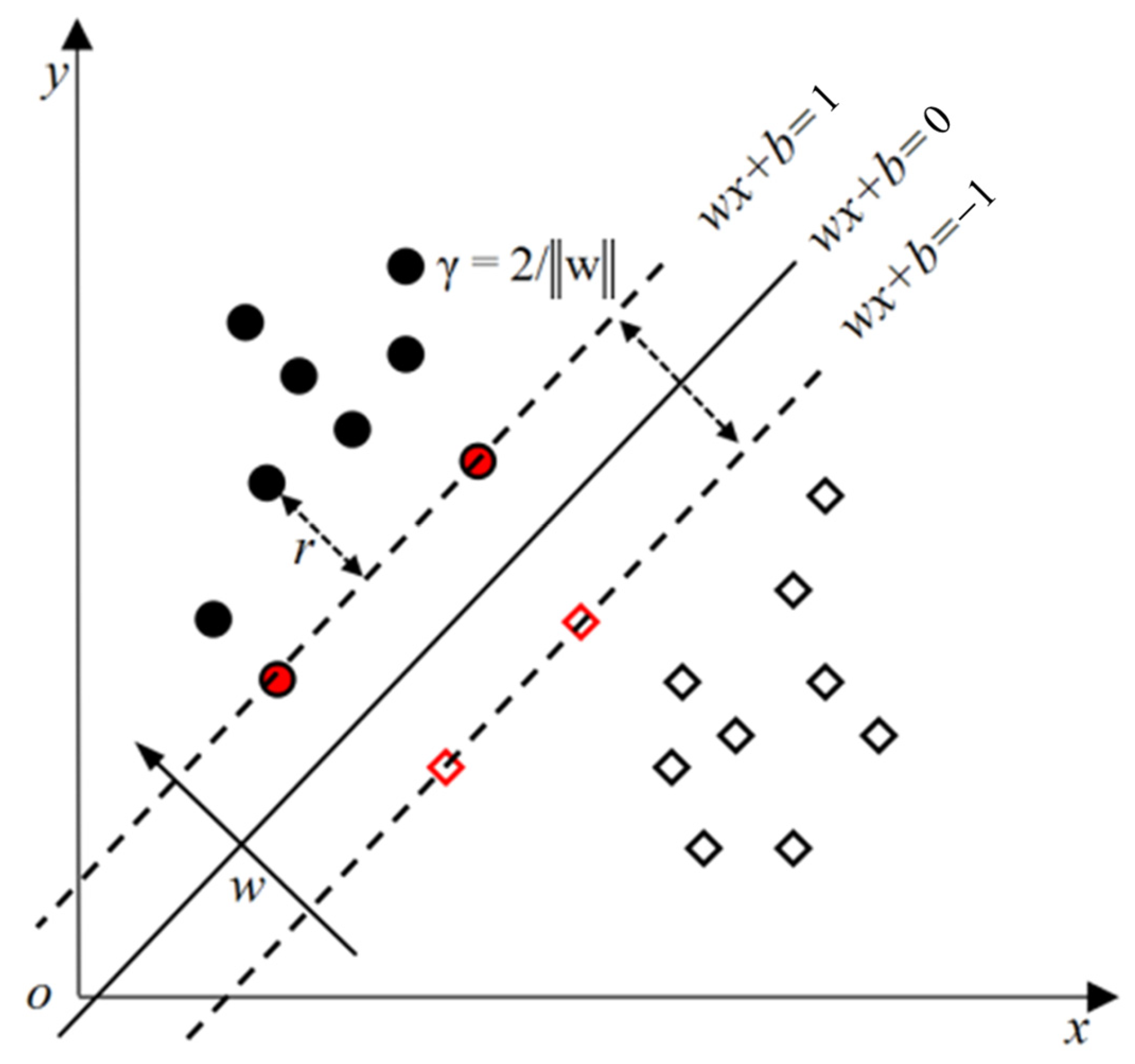
As shown in
Figure 1, for a given training dataset
T in the feature space and hyperplane (
wx +
b = 0) (in which
w is the weight vector and
b is the fitting deviation), the geometric spacing of the hyperplane to the sample point (
xi,
yi) is defined as shown in Equation (1), and the minimum of the geometrical interval of all the hyperplanes about the sample point is shown in Equation (2):
According to Equations (3) and (4), it can be seen that the process of finding the maximum separating hyperplane can be transformed into an optimization problem of maximizing γ under the constraint of minimizing all geometric intervals. This problem is equivalent to finding the minimization
, such that
; the objective function and constraints of this objective function are shown in Equations (3) and (4):
The convex quadratic programming problem with constraints is transformed into a Lagrangian dyadic problem without constraints using the Lagrange multiplier method by attaching a Lagrange multiplier
α to the constraints, and the newly constructed function is shown in Equation (5):
The
L(
w,
b,
ɑ) is, respectively, a partial derivative of
w and
b to 0, and its result is brought back to the original function to obtain a new objective function and constraints, which can be used to find the maximum-margin hyperplane of the training dataset, i.e., the “decision plane”. However, the midspan deflection monitoring data of the main bridge girder cannot be attained in a linearly differentiated manner. Thus, the objective function and constraints under the nonlinearly differentiated dataset are shown in Equations (6) and (7), respectively, through the introduction of the kernel function (
K(
)) and the penalty parameter (
C) to allow specific data points to fail to meet the constraint conditions.
The optimal α* = ()T for the dataset under nonlinearly differentiable conditions can be obtained by the above transformation.
2.2. DIWPSO Algorithm
The particle swarm optimization (PSO) algorithm is a kind of bionic evolutionary computing technology based on bird flock foraging. Its basic idea is to complete the search for optimal solutions through collaborative foraging and information exchange between individuals in the flock, which has the characteristics of a swarm intelligence stochastic search [
30]. The basic principles of PSO algorithms are as follows.
Firstly, a particle with only two attributes of position (
x) and velocity (
v) is assumed in the
D-dimensional vector space to simulate the bird population, in which the velocity attribute represents the individual’s movement speed, and the position attribute represents the individual’s movement direction. All the particles search for the optimal solution individually in the
D-dimensional search space and mark it as the individual’s extreme value; the particles share the information of each other’s extremes to compare the optimal solution and update their own movement speed and movement direction at the same time. The position vector of the
i-th particle is
, and the velocity vector is
; then, the velocity and position updating rule of the standard particle swarm algorithm is shown in Equations (8) and (9):
where
is the inertia factor, the value of which determines the focus of the algorithm on global and local optimization;
is the individual extreme value of the
i-th particle at the
n-th iteration;
is the global extreme value of the population at the nth iteration, where the particles update their velocity and position by keeping track of the individual extreme value and the global extreme value;
and
are the learning factors; and
and
are random numbers in [0, 1].
Generally, the standard PSO algorithm performance is not stable; there are defects of a slow convergence speed, or the standard PSO algorithm might be caught in the local extreme value. This study adopts the improvement method of dynamic inertia weight (DIW) to balance the ability of the PSO algorithm to develop globally and locally search for the optimal [
10]. According to the average aggregation degree and the maximum aggregation degree of the particle swarm in Equations (10) and (11), the rate of change in the aggregation distance (
k) of the particle swarm could be defined as shown in Equation (12).
where
m is the number of particles in the particle swarm population.
The variation rule of inertia weight (
w) is shown in Equation (13).
where
= 0.3,
= 0.2,
rand() is a random number obeying a uniform distribution in [0, 1].
Through Equation (13), the PSO algorithm can take the value of inertia weight (w) at the right time according to the current optimization searching situation, which demonstrates the dynamic adjustment ability of the PSO algorithm to the global search and local development. When the parameter (k) is larger, the maximum spacing in the particle swarm is much larger than the average spacing of the particle swarm, indicating that the aggregation degree of the particle swarm is higher and the global search ability is insufficient. On the contrary, when the parameter (k) is smaller, the inertia weight needs to be adjusted to strengthen the algorithm’s local development ability.
The parameters , , and the inertia weight ω in our dynamic inertia weight PSO (DIWPSO) algorithm were determined through extensive pre-experiments and theoretical analysis to align with the piecewise-function-based regulation logic of ω. Specifically, and serve as foundational scaling coefficients in the piecewise formula, ensuring that ω dynamically balances exploration (global search) and exploitation (local refinement) across different iteration stages. Their values were not independently optimized but were instead selected to support the overall efficacy of the piecewise inertia weight structure. Further fine-tuning of and could be explored in future studies focused on parameter refinement, but their current settings were sufficient to demonstrate the formula’s overall innovation. Regarding the learning factors and , which control the cognitive and social components of particle movement, we adopted the classic setting = = 2, which is a widely accepted default in the PSO literature that balances exploration and exploitation. While dynamic adjustments of and have been proposed in some PSO variants, empirical evidence supports the robustness of fixed values in the base PSO framework, and our study does not innovate these factors. The swarm size (50 particles) and maximum iterations (100) were empirically selected to balance computational cost and convergence stability, with the latter ensuring sufficient optimization without excessive runtime. Together, these parameter choices prioritize the validation of our piecewise inertia weight mechanism over isolated parameter tuning, aligning with the study’s focus on enhancing SVM parameter optimization for structural health monitoring.
2.3. Optimization of SVM Kernel Parameters Based on DIWPSO Algorithm
The relevant parameters of the SVM algorithm can be optimized using the DIWPSO algorithm. The objective function selected in this study is the RMSE function that responds to the performance of the SVM algorithm, of which the function expression is described in Equation (14).
The fitness function is shown in Equation (15).
where the parameter (
C) is the penalty coefficient;
σ is the kernel function parameter;
ε is the error tolerance; and
is the prediction function under the training sample.
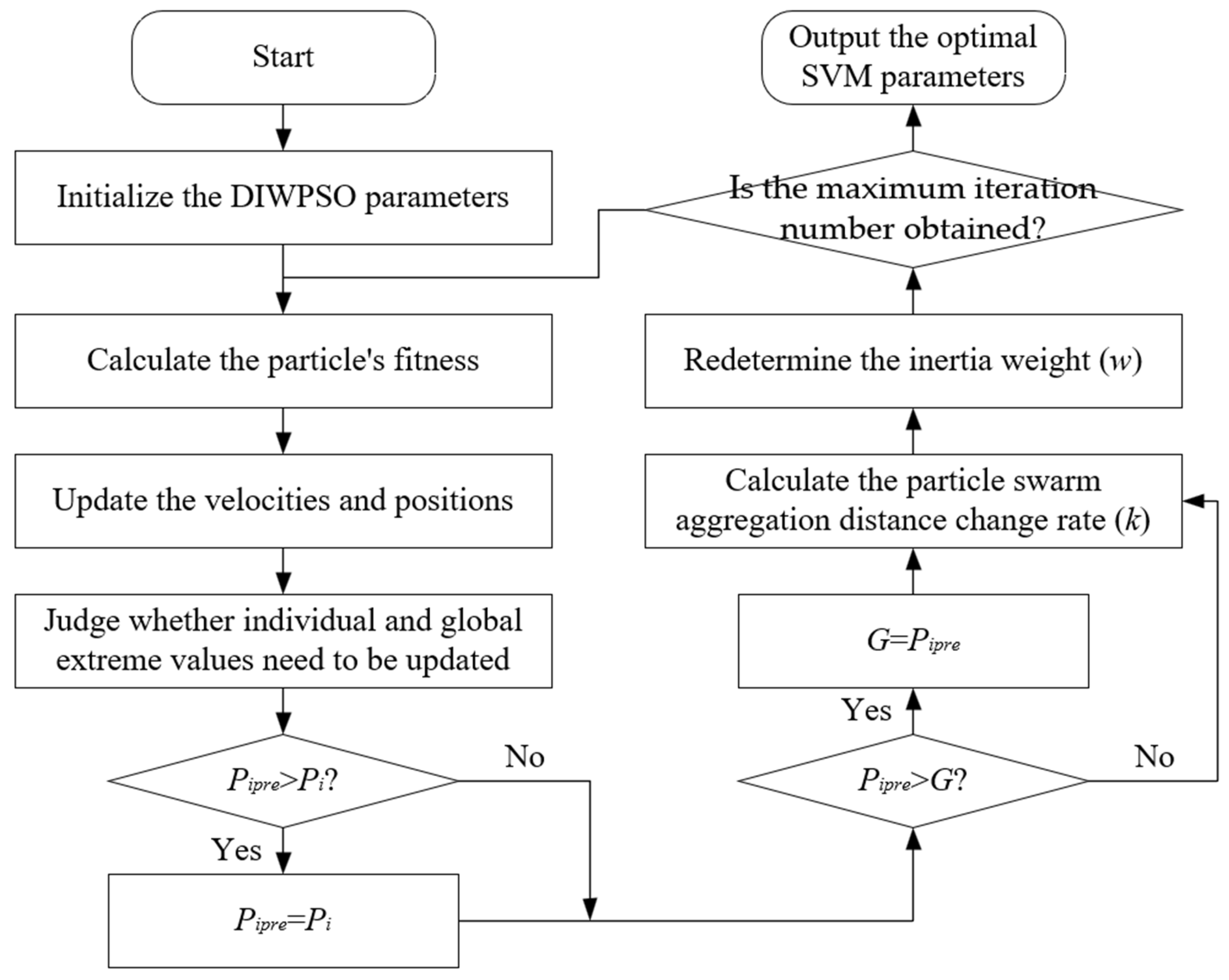
The specific steps for optimizing the kernel function parameters for the SVM algorithm based on the improved DIWPSO algorithm (in
Figure 2) are as follows:
Step (1): Firstly, initialize the DIWPSO algorithm parameters (), the particle swarm size, and the maximal iteration number. Randomly initialize the velocities and positions in the particle swarm of the SVM algorithm parameters () and define the value range of parameters.
Step (2): Update the current position of the particle to the individual extreme value, calculate the particle’s fitness according to Equation (14), and take the particle with the smallest fitness value as the global extreme value.
Step (3): Update the velocities and positions of all particles, make , and compare the individual optimal solutions. If > , update and compare the global optimal solution; if , update .
Step (4): Calculate the particle swarm aggregation distance change rate (k) according to Equation (12), redetermine the inertia weight (w) according to Equation (13), and update and calculate the fitness value.
Step (5): Judge whether the algorithm satisfies the convergence condition; if it does, then output the optimal SVM parameters (). Otherwise, go back to step (2).
Figure 2.
Parameter optimization process of SVM algorithm by DIWPSO.
Figure 2.
Parameter optimization process of SVM algorithm by DIWPSO.
3. A Newly Proposed Midspan Deflection Prediction Based on the DIWPSO-SVM Model Combined with Wavelet Transform Decomposition
3.1. Wavelet Transform-Based Separation of Load Effects
Wavelet transform is an effective analytical method for signal processing with better localization and multiresolution characteristics, which can simultaneously analyze signals in the time and frequency domains, overcoming the shortcomings of the traditional Fourier analysis [
31]. Wavelet transform was initially limited due to drawbacks such as excessive arithmetic. However, the signal was decomposed into detailed and approximate components with the introduction of excellent decomposition algorithms such as Mallat multiresolution analysis. The wavelet transform harmonic extraction method based on the fast algorithm has become a widely used harmonic detection method [
32]. Therefore, the Mallat wavelet transform algorithm was used in this study to deconstruct the mid-span deflection signal.
The vertical deflection of a bridge is mainly affected by the ambient temperature and vehicle load, in which the total response of bridges is obtained under the combined effect of temperature load and vehicle load in usual deflection monitoring. However, the deflection curves of bridges under two kinds of load effects have completely different characteristics. The data under different load effects can be learned and analyzed separately, and then re-stacked, which can improve the prediction accuracy of the SVM algorithm. Therefore, it is necessary to separate the sample data from the load effects.
The effect of temperature load on bridge deflection is mainly classified into annual and daily temperature difference effects, which are measured on time scales of years and days, respectively. The vehicle load is a moving load, and the corresponding vertical deflection is characterized by high-frequency signals measured in seconds. The annual temperature difference effect has the characteristics of a low-frequency signal, which has the most negligible effect on the short-term deflection of the bridge. Thus, the effect of long-term temperature differences on the short-term deflection of bridges was ignored in this study; only the short-term temperature deflection curve and the deflection curve could be extracted for analysis.
In order to accurately analyze the characteristics of the mid-span deflection curves of the main bridge girder under two kinds of load effects, the Mallat wavelet transform algorithm was adopted to deconstruct the mid-span deflection signals [
11]. The basic algorithm of the Mallat wavelet transform is shown in Equation (16).
where
and
are the wavelet coefficients of the signal
f(t) in the low-frequency and high-frequency parts, respectively.
H and
G are the low-pass and high-pass filters of Daubechies six-order (Db6) wavelet basis functions, respectively.
t is the discrete time series, and
j is the number of decomposition layers,
j = 5.
The reconstruction algorithm is shown in Equation (17).
where
h and
g are the reconstructed wavelet low-pass and high-pass filters, respectively.
3.2. Deflection Prediction Process of Midspan Deflection Based on DCWPSO-SVM Model
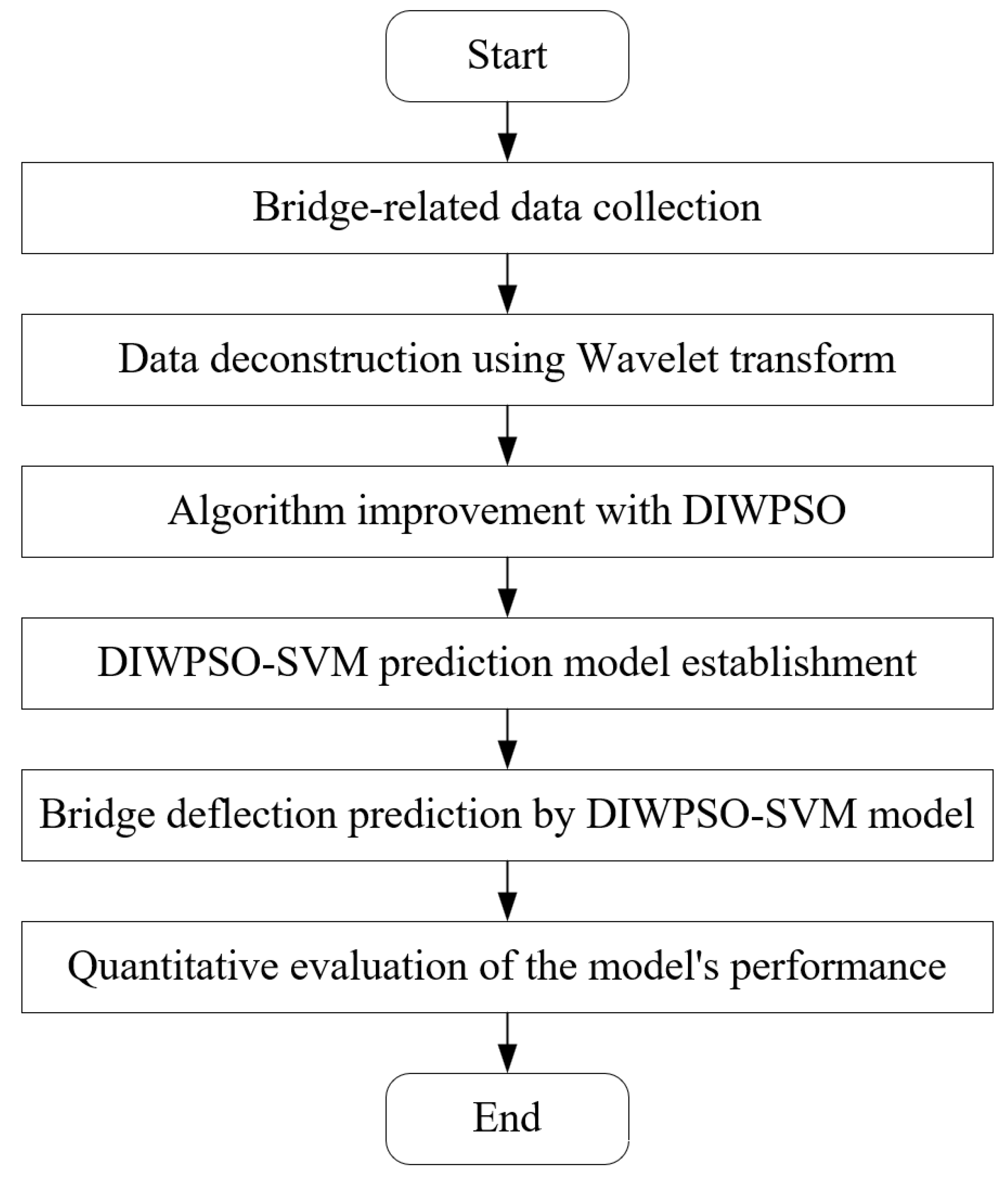
For the accuracy and efficiency of deflection predictions, a hybrid model combining the dynamic inertia weight particle swarm optimization (DIWPSO) with support vector machine (SVM) was established, considering various influencing factors such as vertical deflection signals, ambient temperature, and vehicle load. The deflection prediction process of midspan deflection based on the DCWPSO-SVM model (
Figure 3) is described as follows:
Step (1): Data collection. Midspan essential data from the main bridge girder are collected, including the vertical deflection signals, ambient temperature, and vehicle load, which form the foundation for subsequent analysis and model training. In the collected signals, Savitzky–Golay filtering was applied to suppress high-frequency noise in deflection measurements; the Hampel filter detected and replaced outliers; and KNN estimated missing values by averaging the k nearest temporal neighbors.
Step (2): Wavelet transform and statistical characterization. The vertical deflection signals collected are subjected to wavelet transform to decompose and reconstruct the vertical deflection database of the main girder under temperature load and vehicle load. By statistically characterizing the probability density of the decomposed deflection curves in terms of hours and fitting them with the normal distribution function, the hourly deflection characteristic value with the most significant probability density is identified, which serves as the sampling point for model prediction comparison, ensuring that the model is trained on representative data.
Step (3): Algorithm improvement with DIWPSO. Addressing the instability and convergence issues of the standard PSO algorithm, the DIWPSO algorithm proposes adopting DIW, which enhances the algorithm’s performance by mitigating the risk of slow convergence or falling into local extreme values. The DIWPSO algorithm, thus, provides a more robust optimization framework for parameter tuning in the SVM prediction model.
Step (4): SVM parameter optimization. Utilizing the improved DIWPSO algorithm, the basic parameters of SVMs are optimized, involving iteratively adjusting the SVM to find the optimal combination that maximizes prediction accuracy. The DIWPSO-SVM prediction model combines the strengths of both DIWPSO and SVM for enhanced performance.
Step (5): Bridge deflection prediction. This DIWPSO-SVM model is used to predict the bridge’s midspan deflection based on the optimized parameters and the input data collected in Step (1). The model’s ability to generalize from the training data is crucial for accurate predictions under varying conditions.
Step (6): Model validation and comparison. The DIWPSO-SVM model is validated by comparing the predicted deflection sampling curves with the measured deflection sampling curves. The goodness of fit is assessed using the root-mean-square error (RMSE). This comparison allows for a quantitative evaluation of the model’s performance and enables a comparison with other prediction models. The effectiveness of the DIWPSO-SVM model is determined by improving deflection prediction accuracy.
Figure 3.
Flowchart of midspan deflection prediction based on DIWPSO-SVM model.
Figure 3.
Flowchart of midspan deflection prediction based on DIWPSO-SVM model.
4. Results and Discussion
4.1. Experimental Data
In this study, a double-tower double cable-stayed steel box girder cable-stayed bridge on a highway was taken as an example of experimental engineering, with a span arrangement of (182 + 450 + 182) m. The monitoring points of vertical deflection on the main girder were arranged as shown in
Figure 4.
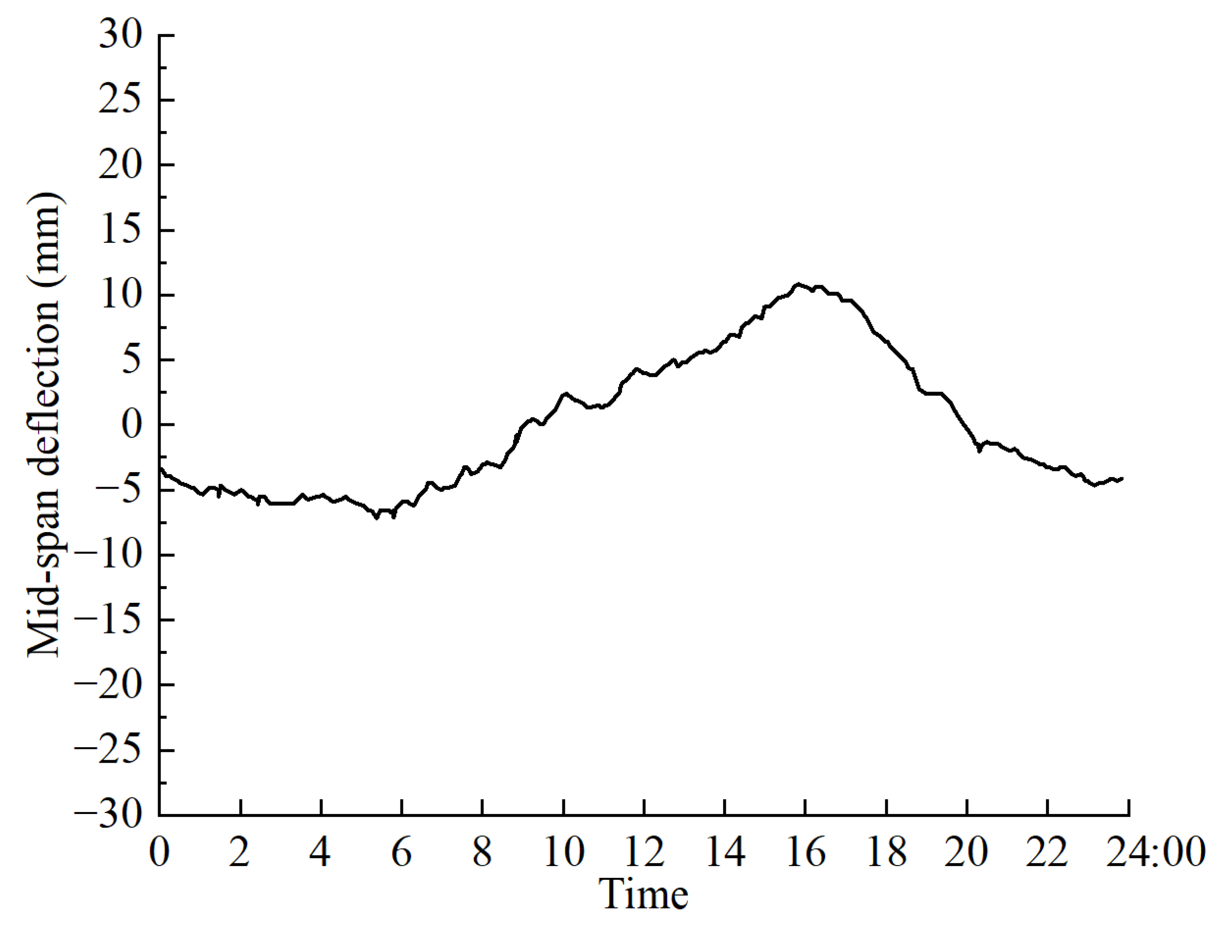
Figure 5 shows the original time–history curve data of the midspan deflection monitoring results during one day on July 1st. It can be seen from
Figure 5 that the monitoring results of vertical deflection have an apparent correlation with the change in ambient temperature. The main girder showed an upward arching trend with a noticeable temperature difference between the upper and lower sections of the main girder when the ambient temperature gradually increased during the daytime. When the ambient temperature gradually decreased at night, there was a decrease in the temperature difference between the upper and lower sections of the main girder, and the vertical deflection of the main girder showed a downward deflection trend.
4.2. Wavelet Transform Decomposition
Mallat wavelet transform was applied to decompose and analyze the deflection curves under temperature load and vehicle load, which provided insights into the temporal variations and magnitudes of deflections in structural elements, such as arches, subjected to different loading conditions.
The deflection time–history curve under temperature load using Mallat wavelet transform decomposition is illustrated in
Figure 6, which reveals critical information regarding the deflections in the upper and lower arches due to temperature variations. Specifically, the maximum deflection in the upper arch, caused by temperature action, occurred approximately at 16:00, with a magnitude of approximately 10 mm. Conversely, the maximum deflection in the lower arch was observed at around 6:00, reaching a magnitude of about 8 mm. These findings highlight the diurnal variations in temperature-induced deflections and their impact on different parts of the arch structure.
Similarly, the deflection time–history curve under vehicle load by Mallat wavelet transform decomposition is shown in
Figure 7. However, the deflection curves exhibit a shorter duration compared to those influenced by temperature variations, which is expected since vehicular loads are typically transient and localized in nature. The peak deflection in the lower arch, concentrated at approximately 5 mm, underscores the impact of vehicular traffic on structural deflection. The concentration of this peak deflection indicates the specific times or conditions under which vehicles contribute most significantly to arch deflection.
The Mallat wavelet transform decomposition technology has proven to be a valuable tool in analyzing and interpreting deflection time–history curves in structural engineering, which is used to identify the temporal patterns and magnitudes of deflections caused by different loading conditions. For instance, the deflection time–history curve under temperature load revealed distinct diurnal patterns; however, the deflection time–history curve under vehicle load demonstrated the transient nature of vehicular impacts.
4.3. Prediction of Midspan Deflection by the DCWPSO-SVM Model
The midspan deflection prediction was carried out using the DIWPSO-SVM model, which was developed and implemented using MATLAB 2016b software, operating on a test platform configured with specific hardware and software specifications. CPU: intel core i5 10400f; RAM: 16 GB; and system version: Windows 10. These hardware and software specifications ensured sufficient computational power to handle the complexity involved in training and validating the predictive models.
To predict the midspan deflection, three different models were employed, including DIWPSO-SVM, PSO-SVM, and SVM, which were trained using sample data from June and subsequently utilized to forecast the midspan deflection for 1 July. A rigorous statistical analysis was conducted on the midspan deflection data collected hourly to validate the effectiveness of these prediction models. Each hourly mid-span deflection data point was subjected to probability density statistics to understand its distribution characteristics. The obtained probability density functions were fitted to a normal distribution. This step assumes that the deflection data follow a normal distribution, which is a common assumption in the statistical analyses of such data. The expected value of the normal distribution was selected as the data sampling point for comparison between measured and predicted values.
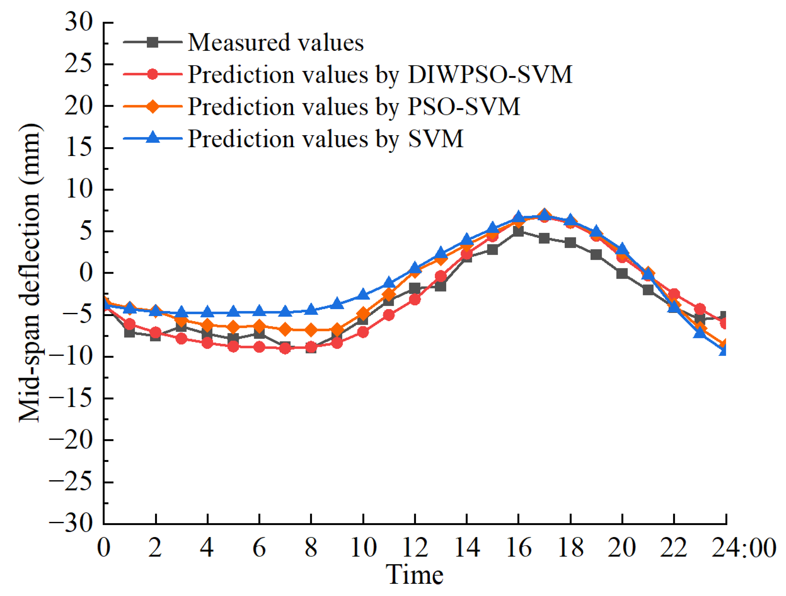
The prediction results are visually presented in
Figure 8, which compares the measured midspan deflection curves with those predicted by the DIWPSO-SVM, PSO-SVM, and SVM models. The SVM model shows the largest deviations from the measured data, while the PSO-SVM model demonstrates good prediction performance but with slightly higher deviations compared to DIWPSO-SVM, reflecting the benefits of PSO. The DIWPSO-SVM model, in particular, offers enhanced performance due to its optimized parameters derived from the improved DIWPSO algorithm. The DIWPSO-SVM model shows the closest alignment with the measured data, indicating high prediction accuracy.
Table 1 presents the prediction errors of different models for midspan deflection. The SVM model optimized with DIWPSO exhibits a significantly better fit to the mid-span deflection data. This optimized model, DIWPSO-SVM, achieves a higher prediction accuracy, with an average error of approximately 1.43 mm and an RMSE of 2.05. The root-mean-square error (RMSE) as a primary metric was used to assess prediction accuracy, which inherently provides a measure of the average prediction error and, thus, is an indication of uncertainty. In contrast, the original SVM model, without optimized parameters, has an average error of around 5.29 mm and an RMSE of 5.62, indicating the lowest prediction accuracy among the models considered. However, the PSO-SVM model, while improving upon the original SVM model, falls short of the DIWPSO-SVM model in terms of prediction accuracy. This suggests that the parameter optimization provided by DIWPSO is more effective than that of PSO in enhancing the predictive capabilities of the SVM model. It is worth noting that the DIWPSO-SVM model requires additional computational time during the initialization stage to iterate the optimization process and determine the optimal parameter combinations for the SVM. Consequently, the total computational time for the DIWPSO-SVM model is higher than that of the original SVM model. However, when considering only the prediction time, it becomes evident that the optimized parameter combinations enable the SVM model to predict more efficiently. Therefore, despite the longer initialization phase, the DIWPSO-SVM model ultimately offers a much lower prediction time compared to the original SVM model. The DIWPSO-SVM model demonstrates superior performance in predicting mid-span deflection, achieving higher accuracy and efficiency through optimized parameter combinations. While the additional computational time required for optimization is a consideration, the overall reduction in prediction time underscores the practicality and effectiveness of this approach.
While the DIWPSO-SVM model’s initialization phase is computationally intensive (approximately 4× longer than the standalone SVM due to PSO-based parameter optimization), this overhead is confined to offline training and does not affect the online prediction efficiency. Consequently, the model may not be suitable for strict real-time applications requiring sub-second responses (e.g., early earthquake warning systems), where latency is critical. However, for near-real-time structural monitoring tasks—such as periodic assessments conducted every 10–30 min—the enhanced accuracy and generalization of DIWPSO-SVM justify the initial delay. Standalone SVMs, while faster to train, often struggle with suboptimal parameter selection in noisy bridge monitoring data, leading to reduced reliability. In contrast, DIWPSO-SVM’s dynamic inertia weight PSO algorithm ensures robustness by escaping local optima and improving long-term predictive performance. This trade-off aligns with industry practices in bridge health monitoring, where minute-level delays are typically acceptable to prioritize reliability over strict latency constraints. Thus, while the increased initialization time limits DIWPSO-SVM’s use in ultra-low-latency scenarios, its advantages in accuracy and generalization make it feasible for near-real-time structural assessments.


