Kolmogorov–Arnold Networks for Reduced-Order Modeling in Unsteady Aerodynamics and Aeroelasticity

Abstract

Kolmogorov–Arnold Networks (KANs) are a recent development in machine learning, offering strong functional representation capabilities, enhanced interpretability, and reduced parameter complexity. Leveraging these advantages, this paper proposes a KAN-based reduced-order model (ROM) for unsteady aerodynamics and aeroelasticity. To effectively capture temporal dependencies inherent in nonlinear unsteady flow phenomena, an architecture termed Kolmogorov–Arnold Gated Recurrent Network (KAGRN) is introduced. By incorporating a recurrent structure and a gating mechanism, the proposed model effectively captures time-delay effects and enables the selective control and preservation of long-term temporal dependencies. This architecture provides high predictive accuracy, good generalization capability, and fast prediction speed. The performance of the model is evaluated using simulations of the NACA (National Advisory Committee for Aeronautics) 64A010 airfoil undergoing harmonic motion and limit cycle oscillations in transonic flow conditions. Results demonstrate that the proposed model can not only accurately and efficiently predict unsteady aerodynamic coefficients, but also effectively capture nonlinear aeroelastic responses.

1. Introduction

In the field of aerospace engineering, accurately predicting aerodynamic and aeroelastic responses is vital for numerous tasks such as system control [1], shape optimization [2], and multifield coupling [3]. High-fidelity computational fluid dynamics (CFD) simulations have become indispensable tools in capturing complex aerodynamic interactions, particularly in scenarios involving flutter [4], transonic buffet [5], and other research in flight mechanics on controllability and stability [6]. However, these CFD techniques require substantial computational resources and prolonged processing durations, restricting their practical utility for iterative design analyses and real-time applications. To address these computational challenges, researchers have increasingly turned to reduced-order models (ROMs), which employ system identification methods [7] based on measured input–output data from the system of interest. Using a concise mathematical expression within a black-box framework, these ROMs capture the essential system behavior while significantly reducing computational costs, thus facilitating real-time or iterative analyses.

However, traditional reduced-order modeling methods frequently exhibit limitations when dealing with strongly nonlinear flow behaviors or intricate transient aerodynamic phenomena. Linear approaches, including AutoRegressive with eXogenous inputs (ARX) [8], AutoRegressive Moving Average (ARMA) [9], and AutoRegressive Integrated Moving Average (ARIMA) [10], have demonstrated notable efficiency in predicting aerodynamic responses but typically fail to accurately represent the complexities associated with nonlinear flow interactions. Although nonlinear polynomial-based methods, such as Wiener and Volterra series expansions [11,12], provide enhanced approximation capabilities, their accuracy and reliability degrade as the system’s nonlinearity and complexity increase.

These limitations underscore a fundamental challenge in aerodynamic modeling: the increasing inadequacy of conventional reduced-order methods when applied to systems with strong nonlinearity, high dimensionality, or unsteady characteristics. This issue becomes particularly pronounced in transonic flow regimes, where shock–boundary layer interactions [13], shock oscillations [14], and other nonlinear wave phenomena [15] introduce substantial complexity. Under such conditions, flow behaviors can exhibit abrupt changes and sensitive dependence on initial or boundary conditions, further straining the capabilities of linear or low-order nonlinear models. With many modern aerodynamic applications operating near transonic speeds, there is a pressing need for more adaptable and robust modeling frameworks that can accurately capture the associated dynamics.

To overcome these limitations, recent advancements have turned towards leveraging machine learning techniques, particularly neural networks, to develop more accurate and efficient reduced-order models. Neural networks have shown great potential in capturing complex, nonlinear relationships inherent in fluid dynamics that traditional ROMs may miss. By training on large datasets generated from high-fidelity CFD simulations, these neural network-based models can learn the intricate patterns and dependencies within the data, enabling them to predict flow behaviors with high precision [16,17]. This approach is bolstered by the ability of data-driven models to generalize across different flow conditions, making them particularly valuable for tasks such as flow control and optimization. In addition, advances in computational resources and algorithmic techniques have facilitated the training of more sophisticated models, further enhancing their predictive capabilities [18].

Accurate prediction of unsteady aerodynamic forces is crucial for both unsteady aerodynamics and aeroelasticity modeling. In essence, aeroelasticity modeling can be regarded as one specific application of unsteady aerodynamic reduced-order modeling. At present, machine learning-based approaches for constructing such models primarily include methods based on radial basis function neural networks (RBFNNs) [19,20], neurofuzzy models [21,22], residual neural networks (ResNets) [23], and deep neural networks (DNNs) [24,25]. Zhang et al. [19] proposed an efficient method for constructing a nonlinear aerodynamic reduced-order model by introducing a recursive structure into the radial basis function neural network (RBFNN), enabling the prediction of limit cycle oscillations. Winter et al. [22] developed a nonlinear system identification strategy by combining a recurrent local linear neurofuzzy model with a multilayer perceptron, thereby enabling accurate and efficient reduced-order modeling of unsteady aerodynamic forces. Qi et al. [23] proposed a reduced-order model based on a residual convolutional neural network within a Nonlinear AutoRegressive model with an eXogenous input (NARX) framework, successfully predicting the strongly nonlinear aerodynamic hysteresis behavior of an airfoil undergoing pitching motion. Li et al. [24] developed a deep neural network-based ROM capable of capturing both unsteady aerodynamic forces and aeroelastic responses over a range of Mach numbers. Despite these advances, existing machine learning-based ROMs still encounter several challenges. In particular, issues related to prediction accuracy under complex nonlinear flow conditions, training stability during model development, and generalization to unseen flow regimes remain unresolved. These limitations underscore the need for further improvements in network architectures to enhance the overall robustness and applicability of data-driven models.

Recently, Kolmogorov–Arnold Networks (KANs) have attracted increasing attention for their ability to learn complex nonlinear mappings with enhanced interpretability and flexibility. Inspired by the Kolmogorov–Arnold representation theorem, KANs replace fixed activation functions with learnable univariate transformations along each edge, enabling the dynamic construction of adaptive basis functions from data [26,27]. This architectural innovation has led to a series of theoretical and algorithmic advancements. Structural improvements include spline-based parameterizations, constrained polynomial representations, and differentiable function modules designed to improve smoothness and numerical stability. Concurrently, researchers have developed gradient regularization techniques, sparsity-promoting constraints, and dynamic pruning methods to reduce overfitting and enhance generalization performance [28]. These innovations have led to strong empirical performance across diverse applications. In symbolic regression, structural refinements, such as the use of monotonic cubic Hermite splines in place of B-splines in KANs, can significantly improve interpretability [29]. In scientific machine learning, KANs have shown strong potential as an alternative to traditional neural architectures by serving as the backbone of neural ODE frameworks. They have demonstrated superior performance in modeling time-dependent and grid-sensitive dynamical systems, achieving higher accuracy, better generalizability, and more efficient parameterization than standard neural networks [30]. In control theory, KANs have been applied to optimal control problems involving continuous-time dynamics, where their integration within the KAN-based framework has demonstrated improved accuracy and efficiency compared to classical MLPs [31]. Moreover, KANs are increasingly being explored for time-series prediction tasks [32,33,34], where capturing temporal dependencies and nonlinear evolution patterns is critical. Recent studies have incorporated KANs into recurrent frameworks, enabling accurate forecasting across a range of sequential data problems. These advancements underscore the suitability of KANs for modeling complex dynamical systems characterized by nonlinear and time-delayed behaviors. In particular, their ability to flexibly represent nonlinear and time-delayed behaviors makes KANs a promising modeling paradigm for unsteady aerodynamics and aeroelastic response prediction, offering new insights into data-driven reduced-order modeling.

This paper introduces a reduced-order model for unsteady aerodynamics and aeroelasticity based on Kolmogorov–Arnold Networks. Inspired by the Temporal Kolmogorov–Arnold Network (TKAN) [32], we developed a novel architecture termed the Kolmogorov–Arnold Gated Recurrent Network (KAGRN) for modeling unsteady aerodynamic forces and nonlinear aeroelastic responses. This innovative structure enables the model to effectively capture the inherent time-delay characteristics and nonlinear dynamics of unsteady aerodynamics, thereby allowing for the accurate identification and prediction of unsteady aerodynamic and aeroelastic behaviors. Furthermore, due to its inherently efficient network structure, the model achieves higher predictive accuracy and improved generalization performance compared to conventional architectures. The effectiveness of the proposed reduced-order model is validated through case studies involving the prediction of unsteady aerodynamic coefficients under harmonic motion, as well as the prediction of limit cycle oscillation (LCO) responses, with results exhibiting strong agreement with those obtained from high-fidelity CFD simulations.

2. Reduced-Order Modeling

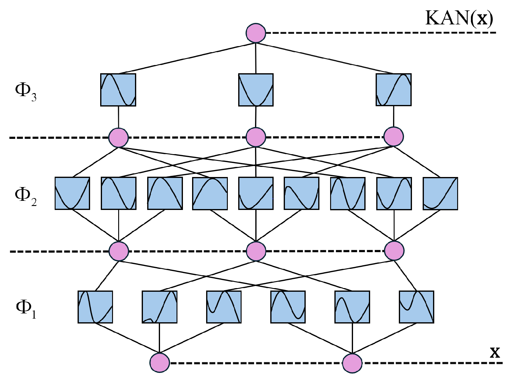
2.1. Kolmogorov–Arnold Networks

Kolmogorov–Arnold Networks (KANs) are a novel neural network architecture based on the Kolmogorov–Arnold representation theorem, which provides a theoretical foundation for expressing multivariate continuous functions through compositions of univariate functions. This enables the decomposition of complex functions into simpler and more interpretable components, making KANs highly effective for function approximation. Figure 1 illustrates the architecture of Kolmogorov–Arnold Networks. According to the Kolmogorov–Arnold theorem, any continuous multivariate function can be expressed as a combination of finite univariate functions, as shown by the following equation:

$$f\left(\mathbf{x}\right)=f(x_1,\dots ,x_n)=\sum _{q=1}^{2n+1}{\mathsf{\Phi }}_q\left(\sum _{p=1}^n{\varphi }_{q,p}\left(x_p\right)\right)$$

(1)

where ${\varphi }_{q,p}\left(x_p\right)$ represents a univariate function defined on each input variable $x_p$, while ${\mathsf{\Phi }}_q$ is responsible for combining these univariate functions into the final approximation.

KANs leverage this theoretical property by parameterizing a set of functions, replacing conventional linear weights in neural networks with univariate functions represented by spline curves. In contrast to traditional multilayer perceptrons (MLPs), which utilize predefined activation functions at their nodes, KANs introduce adaptive activation functions on the connections between nodes. These activations, modeled using B-spline parameterizations, are capable of adjusting dynamically throughout training to more accurately model the underlying data characteristics. Formally, a KAN layer with $n_{\mathrm{in}}$-dimensional inputs and $n_{\mathrm{out}}$-dimensional outputs can be expressed as an array of one-dimensional functions $\mathsf{\Phi }=\left\{{\varphi }_{q,p}\right\}$, indexed by $p=1,2,\dots ,n_{\mathrm{in}}$ and $q=1,2,\dots ,n_{\mathrm{out}}$. Each function ${\varphi }_{q,p}$ is characterized by parameters that are optimized during the training process. Extending this concept to practical implementations, KAN architectures typically adopt a multilayer structure, where each layer sequentially applies transformations inspired by the Kolmogorov–Arnold representation. Consequently, the overall mapping from input to output in a multilayer KAN model can be succinctly expressed through function composition as

$$\mathrm{KAN}\left(\mathbf{x}\right)=\left({\mathsf{\Phi }}_{L-1}\circ {\mathsf{\Phi }}_{L-2}\circ \dots \circ {\mathsf{\Phi }}_1\circ {\mathsf{\Phi }}_0\right)\mathbf{x}$$

(2)

where each ${\mathsf{\Phi }}_l$ corresponds to a distinct KAN layer. This layered architecture not only retains the hierarchical structure characteristic of conventional neural networks but also offers exceptional nonlinear approximation capabilities, making KAN particularly effective for complex data modeling and analytical tasks.

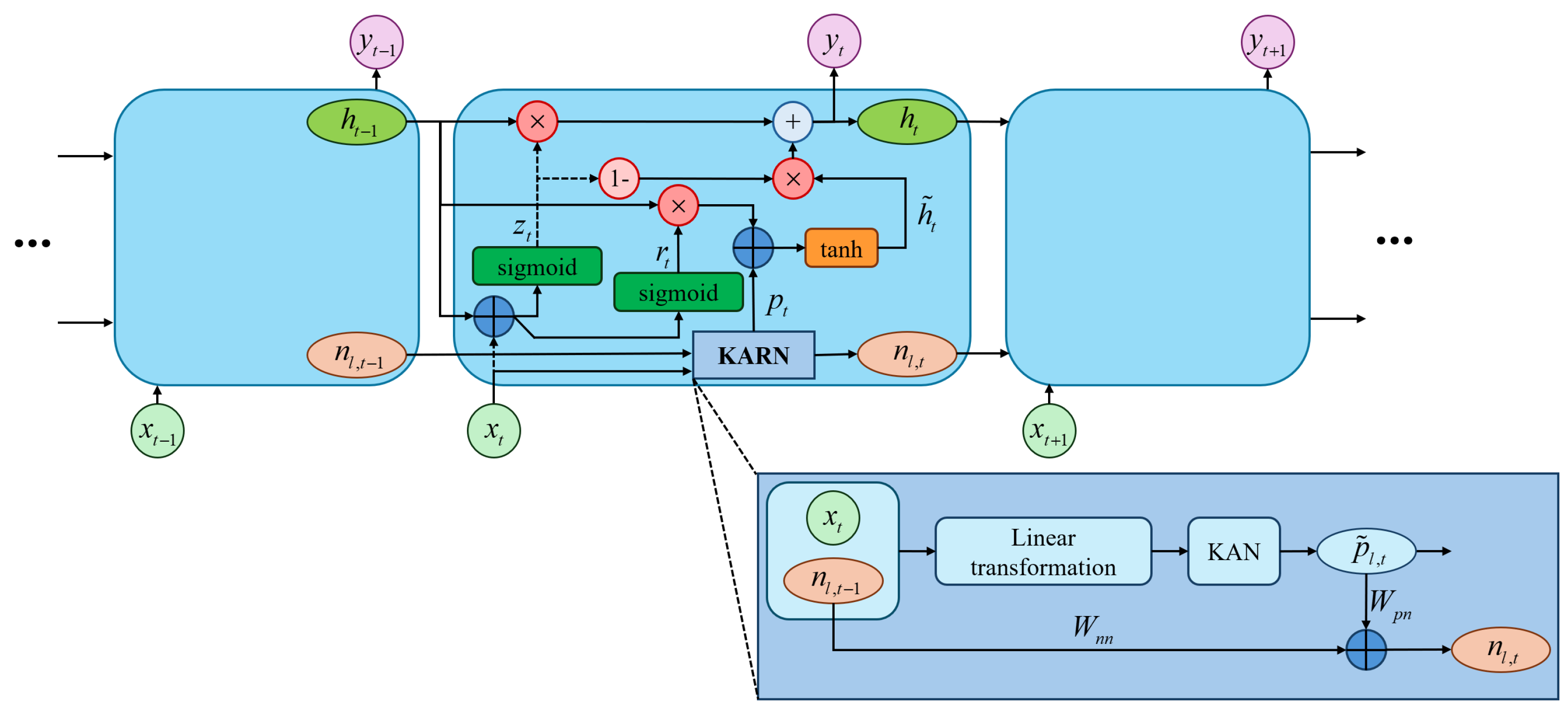
2.2. Kolmogorov–Arnold Gated Recurrent Networks

The Kolmogorov–Arnold Gated Recurrent Network (KAGRN) represents an advanced recurrent neural network architecture designed to effectively capture complex temporal dynamics. The network primarily consists of two components: the Kolmogorov–Arnold Recurrent Network (KARN) layers and the gating mechanisms inspired by Gated Recurrent Units (GRUs). Specifically, KARN layers utilize learnable activation functions based on the Kolmogorov–Arnold representation theorem to accurately capture complex nonlinearities, while the gating mechanisms selectively control and maintain long-term temporal dependencies. The architecture of Kolmogorov–Arnold Gated Recurrent Networks is shown in Figure 2. Inspired by the Temporal Kolmogorov–Arnold Network (TKAN) [32], we develop this architecture to effectively model intricate temporal relationships inherent in aerodynamic data, enabling the accurate identification and prediction of unsteady aerodynamic and aeroelastic behaviors.

To clearly illustrate the proposed architecture, Figure 2 further details the internal structure of the KARN layers, highlighting their mathematical formulation and computational flow. The KARN is designed specifically to model sequential data, capturing context-sensitive dependencies through an integration of Kolmogorov–Arnold Networks and memory-based recurrence mechanisms. KARN modifies each transformation function ${\phi }_l$ within the traditional KAN architecture by embedding a temporal dimension. Formally, the input to each recursive sublayer at time t is expressed by the following relation:

$$i_{l,t}=W_{l,x}{x}_t+W_{l,n}{n}_{l,t-1}$$

(3)

where $W_{l,x}$ and $W_{l,n}$ denote the weight matrices connecting current inputs $x_t$ and previous memory states $n_{l,t-1}$, respectively. Given that the dimensions of the input and output in layer l are $KA{N}_{in}$ and $KA{N}_{out}$, the associated weight matrices have dimensions $W_{l,x}\in {\mathbb{R}}^{(d,KA{N}_{in})}$ and $W_{l,n}\in {\mathbb{R}}^{(KA{N}_{out},KA{N}_{in})}$. Each transformed sublayer state $i_{l,t}$ is then passed through a nonlinear KAN function as

$${\tilde{p}}_{l,t}={\phi }_l\left(i_{l,t}\right)$$

(4)

where ${\tilde{p}}_{l,t}$ represents the nonlinear transformed output at time t. Furthermore, the model incorporates a recurrent memory mechanism update expressed by the following equation:

$$n_{l,t}=W_{nn}{n}_{l,t-1}+W_{pn}{\tilde{p}}_{l,t}$$

(5)

where $n_{l,t}$ represents the updated hidden memory state at layer l and time t. Specifically, $n_{l,t}$ encapsulates the learned latent representations retained and refined across time steps. In this recurrence, $W_{nn}$ serves to propagate and maintain previous hidden states, while $W_{pn}$ integrates the current nonlinear outputs into the evolving memory states. This design effectively enables the network to capture temporal dependencies by dynamically adjusting and propagating past latent representations across time steps.

Gating mechanisms are known to effectively control the propagation of information across time steps, significantly improving a neural network’s capability to capture long-term dependencies and mitigating issues such as vanishing or exploding gradients commonly encountered in recurrent structures. Building upon the strengths of the KARN layers, we further incorporate gating mechanisms inspired by Gated Recurrent Units to develop the Kolmogorov–Arnold Gated Recurrent Network. Given an input vector $x_t\in {\mathbb{R}}^d$, the update gate $z_t$ and reset gate $r_t$ are computed at each time step t as follows:

$$z_t=\sigma (W_z{x}_t+U_z{h}_{t-1}+b_z),r_t=\sigma (W_r{x}_t+U_r{h}_{t-1}+b_r)$$

(6)

where $W_r,W_z$ and $U_r,U_z$ represent corresponding weight matrices, and $b_z,b_r$ represent corresponding bias vectors. The function $\sigma (·)$ denotes the activation function, which is set to the sigmoid function in this work. The vector $p_t$ is defined as the concatenation of outputs obtained from multiple KAN layers, formally expressed as follows:

$$p_t=\mathrm{Concat}[{\tilde{p}}_{1,t},{\tilde{p}}_{2,t},\dots ,{\tilde{p}}_{L,t}]$$

(7)

Subsequently, the candidate hidden state ${\tilde{h}}_t$ is computed via

$${\tilde{h}}_t=tanh(W_h{p}_t+U_h(r_t\odot h_{t-1})+b_h)$$

where ${\tilde{h}}_t$ represents the internal memory state. Finally, the hidden state $h_t$ is updated according to the following equation:

$$h_t=z_t\odot h_{t-1}+(1-z_t)\odot {\tilde{h}}_t$$

(8)

Through this design, KAGRN combines KARN with gating mechanisms, where the Kolmogorov–Arnold recurrent layers provide enhanced nonlinear representational capabilities essential for modeling complex input–output relationships, and the gating mechanisms effectively mitigate vanishing gradients and dynamically manage information flow, enabling the network to better capture and retain long-term temporal dependencies. This innovative architecture exhibits superior generalization performance compared to conventional approaches while maintaining robust modeling capabilities, allowing for a more accurate and efficient representation of the dynamic characteristics inherent in unsteady aerodynamics and aeroelasticity.

In addition to its ability to represent complex unsteady aerodynamic characteristics with high accuracy, KAGRN also offers a distinctive interpretability advantage that is particularly valuable in the context of reduced-order modeling. Within this setting, the KAN sublayer provides an explicit functional decomposition: each learned one-dimensional mapping can be analyzed independently, enabling practitioners to directly understand how specific displacement components influence the predicted aerodynamic force coefficients. The shapes of these mappings often reveal physically meaningful nonlinear behaviors that would remain obscured in conventional black-box models. In this sense, the KAN serves as a compact, data-driven basis that maps structural motion to aerodynamic response in a more transparent and physically interpretable manner than conventional approaches.

Together, these attributes demonstrate that KAGRN not only achieves high predictive accuracy but also enhances model transparency, offering valuable insights into the underlying dynamics. This combination of accuracy and interpretability makes KAGRN particularly suited for scientific analysis and engineering deployment.

2.3. Unsteady Aerodynamic and Aeroelasticity Modeling

In this work, we employ the proposed KAGRN framework to model unsteady aerodynamics and aeroelasticity. Specifically, the input and output vectors at time step t are defined as follows:

$$\begin{array}{cc}\hfill x_t& =\left[\begin{array}{cc}{(h/b)}_t& {\alpha }_t\end{array}\right]\hfill \\ \hfill y_t& =\left[\begin{array}{cc}{\left(C_l\right)}_t& {\left(C_m\right)}_t\end{array}\right]\hfill \end{array}$$

(9)

where h denotes the plunging displacement, b represents the semi-chord length, $\alpha$ is the pitching angle, and $C_l$ and $C_m$ correspond to the lift and pitching moment coefficients, respectively. Unlike conventional nonlinear reduced-order modeling approaches, such as the Nonlinear AutoRegressive models with eXogenous input (NARX) framework [19,22,23], our proposed method explicitly introduces hidden state representations to capture the intrinsic time-delay characteristics associated with unsteady aerodynamic responses. This approach not only improves the accuracy of the model, but also significantly enhances its generalizability across various aerodynamic conditions, particularly when handling nonlinearities and complex transient phenomena.

Figure 3 illustrates the flowchart for training and application procedures of the proposed reduced-order model (ROM). In this study, the ROM is trained using stochastic motion data as inputs, while the corresponding aerodynamic coefficients, obtained from computational fluid dynamics (CFD) simulations, serve as the outputs. A detailed description of the training procedure and model parameters is provided in Section 4.1. After successful training, the ROM can be applied for the following purposes:

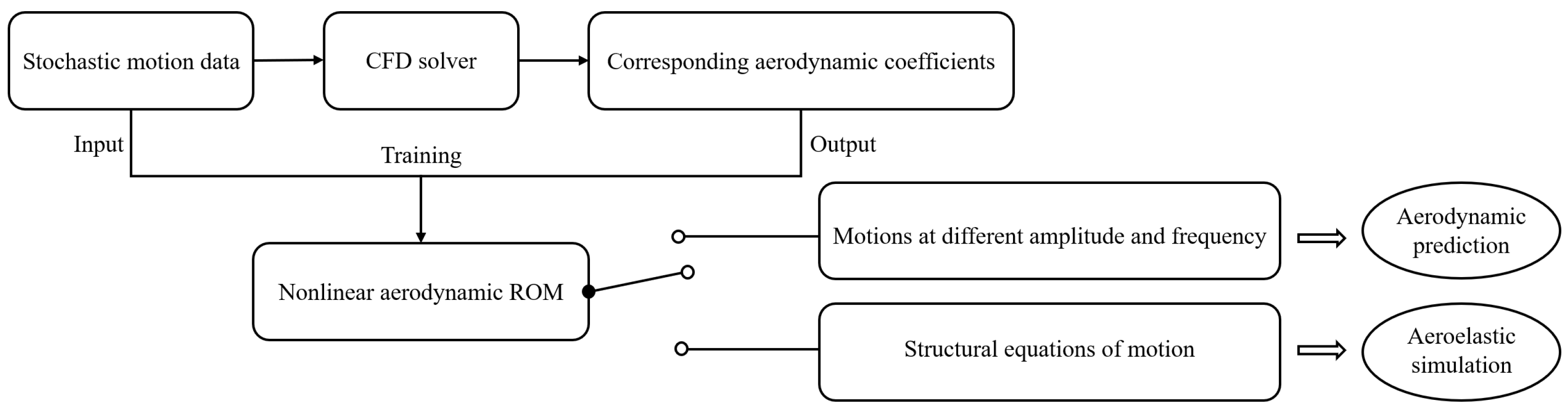
• Aerodynamic prediction: Given the prescribed structural motions as input, the trained ROM predicts the corresponding nonlinear and unsteady aerodynamic coefficients.
• Aeroelastic simulation: Given the nonlinear aerodynamic ROM and the structural equations of motion, a loosely coupled aeroelastic simulation strategy is employed. Specifically, at each time step, the trained ROM predicts the aerodynamic coefficients, which are then used to update the structural response through the structural equations of motion before advancing to the next time step.

3. Numerical Method

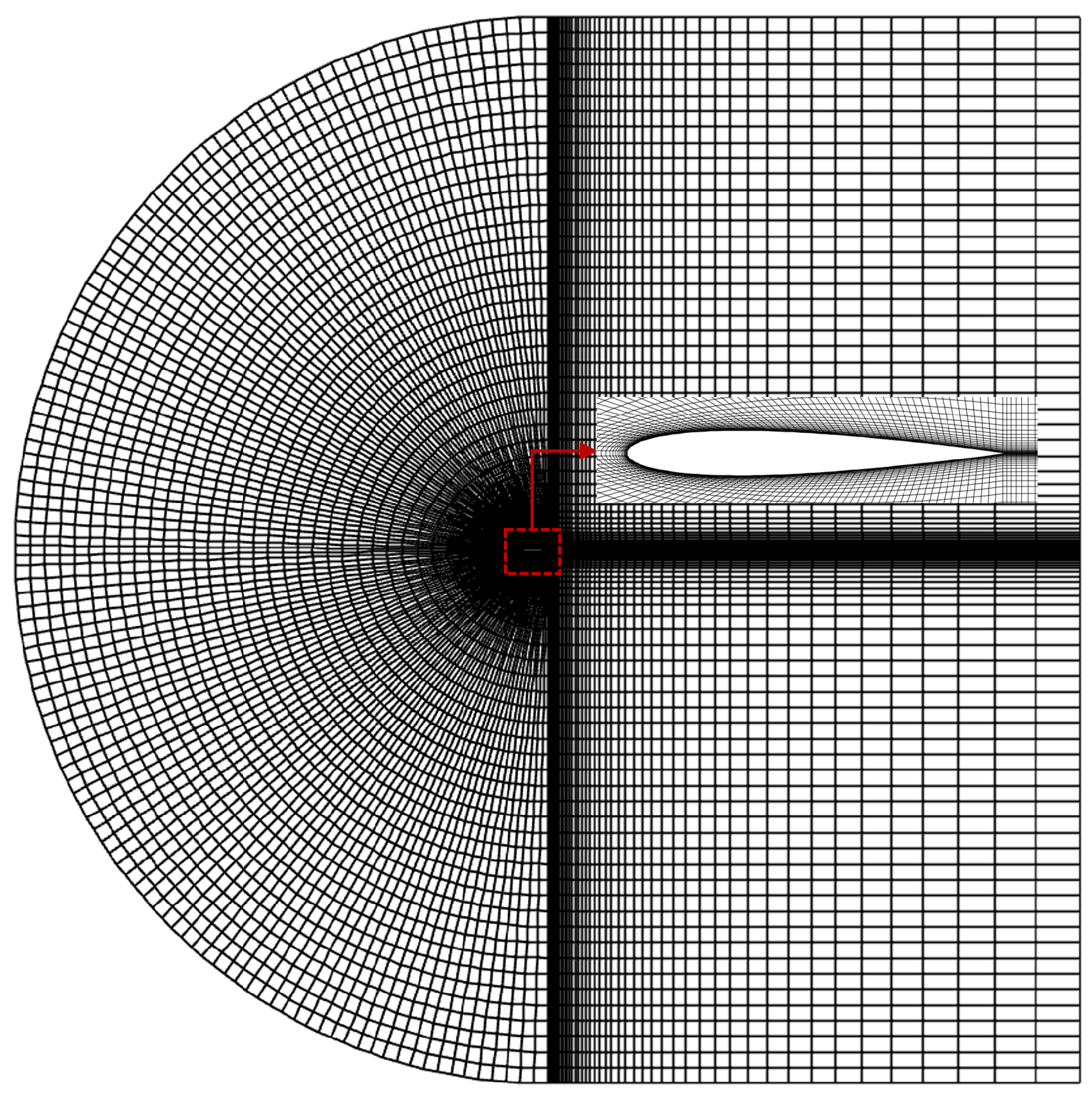
3.1. CFD Solver

In this study, we employ an unsteady flow solver to numerically solve the Euler equations and the Reynolds-averaged Navier–Stokes (RANS) equations. In a Cartesian coordinate system, the unsteady Reynolds-averaged Navier–Stokes equations can be expressed in the integral form as

$${\displaystyle \frac{\partial }{\partial t}}\underset{\mathsf{\Omega }}{\int \int \int }\mathbf{W}dV+\underset{\partial \mathsf{\Omega }}{\int \int }{\mathbf{F}}^i\left(\mathbf{W}\right)·\mathbf{n}dS=\underset{\partial \mathsf{\Omega }}{\int \int }{\mathbf{F}}^v\left(\mathbf{W}\right)·\mathbf{n}dS$$

(10)

where $\mathsf{\Omega }$ denotes the control volume, while $\partial \mathsf{\Omega }$ represents its boundary. The vector n is the outward-pointing unit normal to the control volume boundary. V represents the volume of the element, and S denotes the area of each face. The variable W corresponds to the conserved variables, while $F^i\left(W\right)$ and $F^v\left(W\right)$ represent the inviscid and viscous fluxes, respectively.

The finite-volume method is utilized to solve the governing equations. In this work, the Euler equations serve as the governing equations. The spatial discretization utilizes a second-order Upwind Roe scheme. For time integration, a dual-time stepping approach is employed, with the implicit LU-SGS method used to solve the discretized equations. The developed solver has been validated through various steady and unsteady flow cases, including flutter scenarios. Further details of the numerical method can be found in [35].

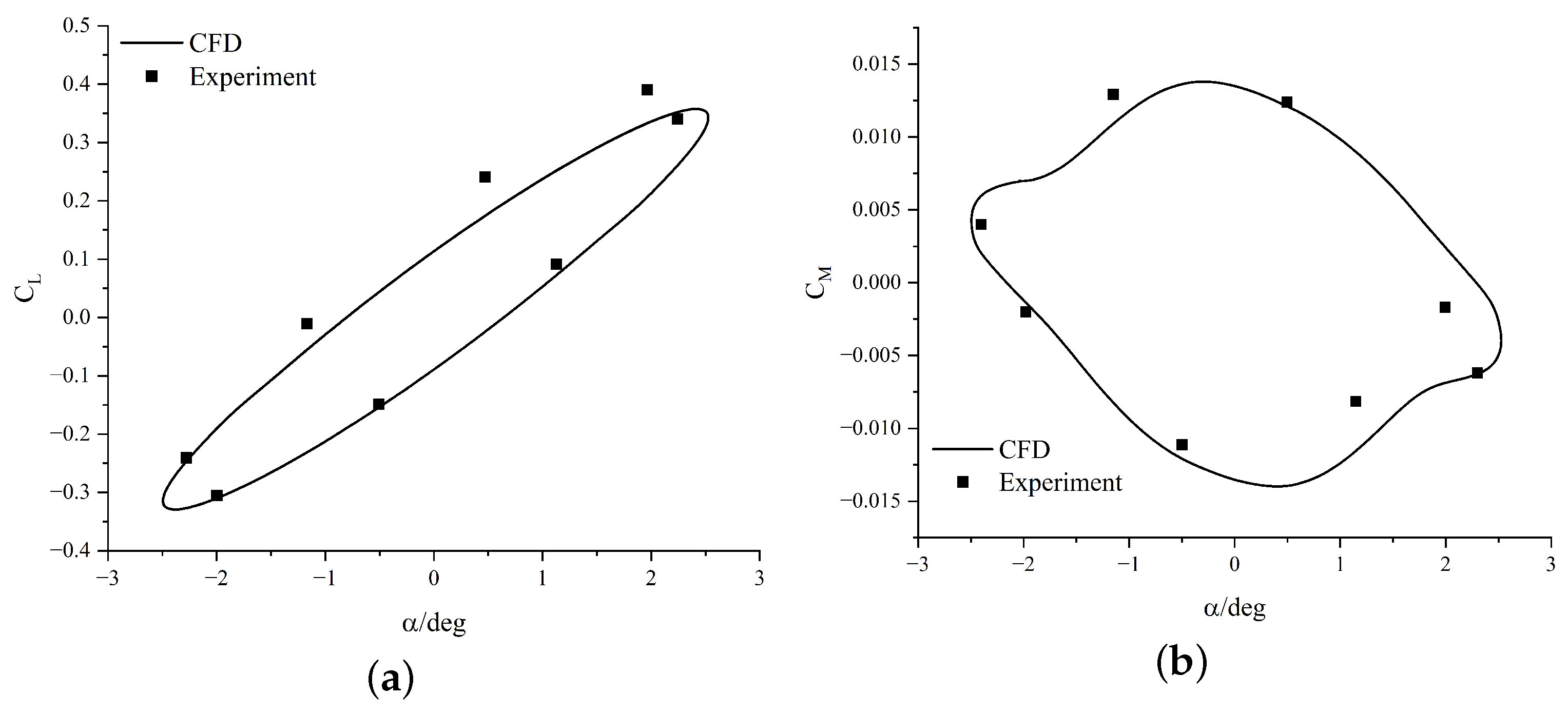
3.2. Method Validation

The AGARD CT5 benchmark [36] is used to verify the accuracy of the CFD solver. This benchmark involves an NACA0012 airfoil subjected to single-degree-of-freedom pitching oscillation. The pitching motion can be described by the following equation:

$$\alpha \left(t\right)={\alpha }_m+{\alpha }_{0}sin\left(\omega t\right)$$

(11)

where $\alpha \left(t\right)$ represents the angle of attack, ${\alpha }_m$ is the mean angle of attack, ${\alpha }_0$ denotes the amplitude of the pitch oscillations, $\omega$ is the angular frequency of the pitch oscillations, and k is the reduced frequency, defined as $k={\displaystyle \frac{\omega c}{2U_{\infty }}}$. In this context, c is the chord length, and $U_{\infty }$ denotes the free-stream velocity. The pitching motion occurs around the quarter-chord point. The computational parameters are ${\alpha }_m=0.{016}^{\circ }$, ${\alpha }_0=2.{51}^{\circ }$, $Ma=0.755$, $Re=5.5\times {10}^6$, and $k=0.0814$.

The computational grid utilizes a C-type structured mesh with 14,818 cells, as shown in Figure 4.

The numerically computed hysteresis loops of the lift and moment coefficients are compared with the experimental values provided by AGARD CT5 [36], as shown in Figure 5. The results indicate a good agreement between the CFD-calculated values and the experimental data, which confirms the accurate predictive capabilities of the unsteady flow solver used in this study.

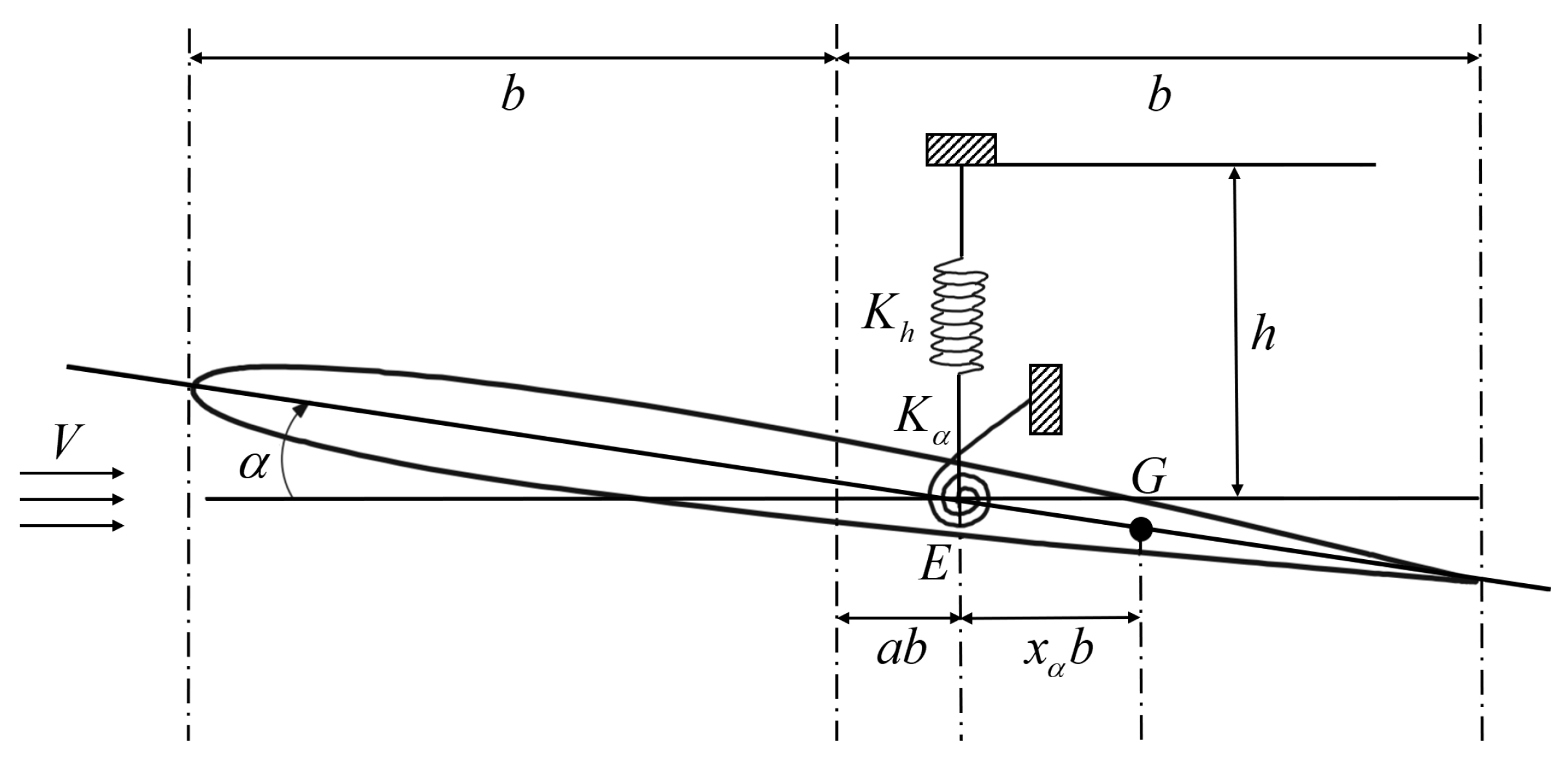
3.3. Structural Equations of Motion

Figure 6 illustrates the aeroelastic model of two degrees of freedom (Isogai Wing model), originally proposed by Isogai [37]. Incorporating both plunging and pitching motions, this model is widely used as a benchmark for two-dimensional transonic aeroelastic studies. It represents a large-aspect-ratio transonic aft-swept wing, where the outboard section undergoes bending and torsion. In this model, the elastic axis E is located $ab$ behind the mid-chord, while the center of gravity G is positioned $x_{\alpha }b$ aft of the elastic axis, where b represents the semi-chord length. The elastic stiffness coefficients associated with plunging and pitching are given by $K_h$ and $K_{\alpha }$, respectively. Based on the Lagrangian formulation, the structural equations of motion for this model can be expressed as follows:

$$\begin{array}{cc}\hfill m\ddot{h}+S_{\alpha }\ddot{\alpha }+K_{h}h& =-L\hfill \\ \hfill S_{\alpha }\ddot{h}+I_{\alpha }\ddot{\alpha }+K_{\alpha }\alpha & =M\hfill \end{array}$$

(12)

where h and $\alpha$ represent the plunging and pitching motions, respectively. m denotes the mass per unit span, while $S_{\alpha }=m{x}_{\alpha }b$ is the static moment about the elastic axis. $I_{\alpha }=m{r}_{\alpha }^2{b}^2$ is the mass moment of inertia about the elastic axis, with $r_{\alpha }$ denoting the dimensionless radius of gyration relative to the elastic axis. L and M represent the aerodynamic lift and the aerodynamic moment about the elastic axis, respectively.

By introducing the dimensionless time variable $\tau ={\omega }_{\alpha }t$, Equation (12) can be rewritten as

$$\left[\begin{array}{cc}1& x_{\alpha }\\ x_{\alpha }& r_{\alpha }^2\end{array}\right]\left\{\begin{array}{c}\ddot{h}/b\\ \ddot{\alpha }\end{array}\right\}+\left[\begin{array}{cc}{\left({\displaystyle \frac{{\omega }_h}{{\omega }_{\alpha }}}\right)}^2& 0\\ 0& r_{\alpha }^2\end{array}\right]\left\{\begin{array}{c}h/b\\ \alpha \end{array}\right\}={\displaystyle \frac{1}{\pi }}{\left(V_f\right)}^2\left\{\begin{array}{c}-C_l\\ 2C_m\end{array}\right\}$$

(13)

where the notation $\ddot{\left(\right)}$ represents the second derivative with respect to $\tau$, i.e., $\ddot{\left(\right)}={\displaystyle \frac{d^2\left(\right)}{d{\tau }^2}}$; and ${\omega }_h=\sqrt{K_h/m}$ and ${\omega }_{\alpha }=\sqrt{K_{\alpha }/I_{\alpha }}$ represent the uncoupled natural frequencies of the plunging and pitching motions, respectively. The dimensionless flutter speed is given by $V_f={\displaystyle \frac{V}{{\omega }_{\alpha }b\sqrt{\mu }}}$, while the mass ratio is defined as $\mu ={\displaystyle \frac{m}{\rho \pi b^2}}$, where V denotes the free-stream velocity and $\rho$ represents the free-stream density. Additionally, $C_l={\displaystyle \frac{L}{\rho V^{2}b}}$ and $C_m={\displaystyle \frac{M}{2\rho V^2{b}^2}}$ denote the lift and moment coefficients, respectively. This system can be efficiently solved using a fourth-order Runge–Kutta method, and more details of the numerical implementation can be found in [35].

4. Results and Discussion

To validate the effectiveness and accuracy of the proposed reduced-order model based on Kolmogorov–Arnold Networks, this study first describes the training procedure and the primary associated parameters of the ROM. Subsequently, the ROM is applied to predict nonlinear unsteady aerodynamics at varying amplitudes and reduced frequencies, and the results are compared against those obtained from computational fluid dynamics simulations. Furthermore, the ROM is coupled with the structural equations of motion to predict the responses of limit cycle oscillations (LCOs), and these predictions are validated by comparing them with corresponding CFD results. Finally, a comparative analysis of predictive accuracy and computational efficiency among different approaches is conducted to evaluate their overall performance.

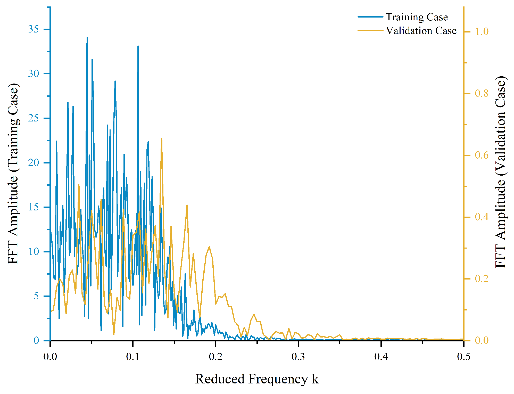
4.1. Training of Reduced-Order Model

The choice of input signal significantly influences the accuracy and generalizability of the reduced-order model, necessitating a random excitation that encompasses a broad frequency spectrum and amplitude variations [18]. In this study, we employ filtered white Gaussian noise (FWGN) signals as inputs for both the training and validation datasets, as illustrated in Figure 7, where T represents discrete time steps. Specifically, the training dataset comprises 5000 time steps with relatively large amplitudes, whereas the validation dataset consists of 2000 time steps featuring smaller amplitudes. The smaller-amplitude input utilized in the validation set is intentionally chosen to rigorously assess and enhance the model’s generalization capabilities across varying input conditions. Additionally, the spectral content of these signals is examined using Fast Fourier Transform (FFT) analysis to confirm adequate frequency coverage, as presented in Figure 8.

Subsequently, the generated input signals at each discrete sampling point are processed through the CFD solver to obtain the corresponding aerodynamic coefficients, thereby establishing comprehensive input–output (I/O) pairs. These resulting I/O datasets serve as the fundamental building blocks for developing the training and validation datasets, thus providing a robust basis for constructing and evaluating the reduced-order model described previously.

The sliding window technique is a prevalent preprocessing strategy for sequential data, particularly beneficial in time-series modeling applications [38]. This method involves segmenting the original sequential dataset into multiple overlapping subsequences of fixed length, thereby explicitly capturing temporal dependencies inherent within the data. Halder et al. [39] successfully employed the sliding window approach to preprocess input data for gust response modeling, significantly improving predictive accuracy. Inspired by their results, we also adopt this technique to systematically organize our sequential input data. This structured preprocessing effectively preserves the temporal dynamics inherent in the original dataset, enabling the proposed KAN-based reduced-order model to capture temporal dependencies more accurately, thereby significantly enhancing predictive accuracy and overall model performance.

In this work, the model was trained using the backpropagation-through-time (BPTT) algorithm, a widely adopted method for optimizing sequential neural networks. To enhance training efficiency and reduce the likelihood of convergence to local minima, the Adam optimizer, which adaptively adjusts learning rates during the optimization process, was employed to minimize the mean-squared error (MSE) loss between predicted and actual aerodynamic coefficients. Furthermore, a validation set was explicitly established during training to regularly assess the model’s predictive performance on unseen data, thereby improving the generalization capability and robustness of the model. The trained model comprises two hidden layers, each with 32 units.

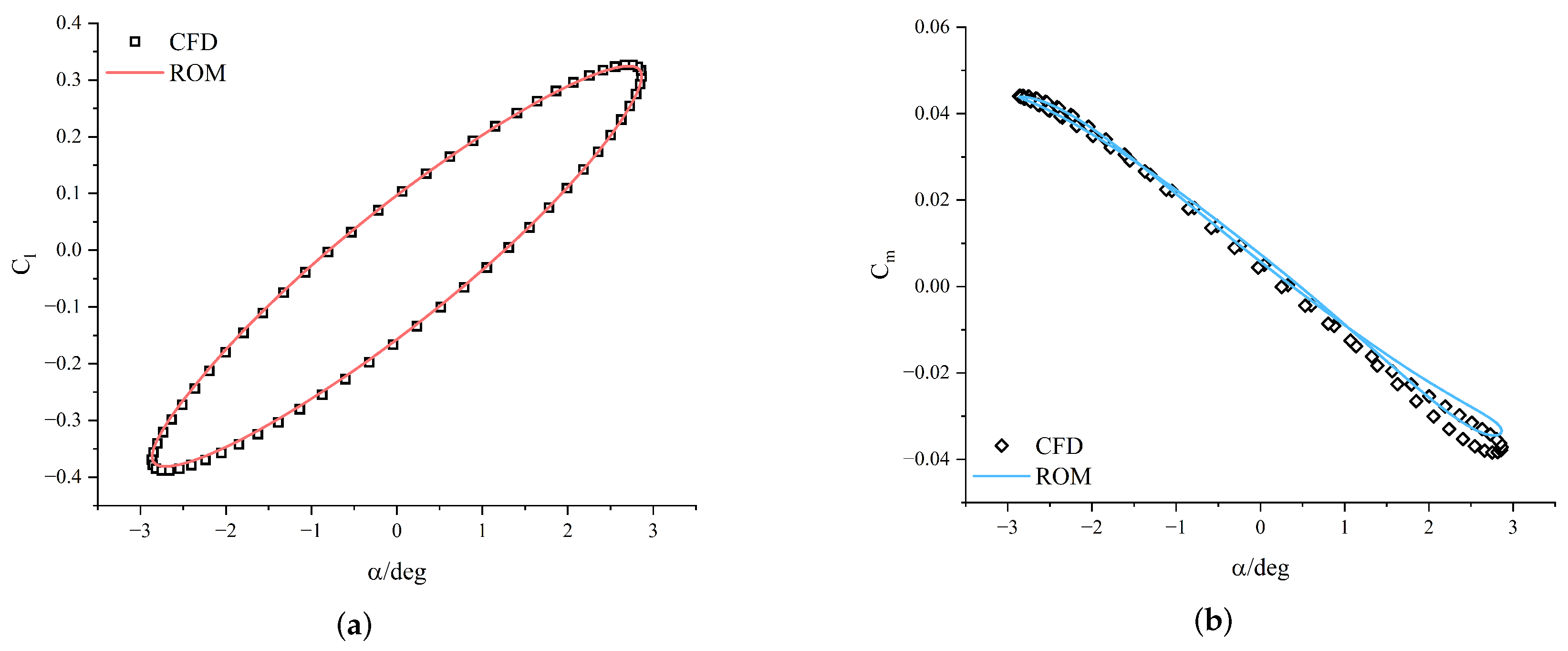
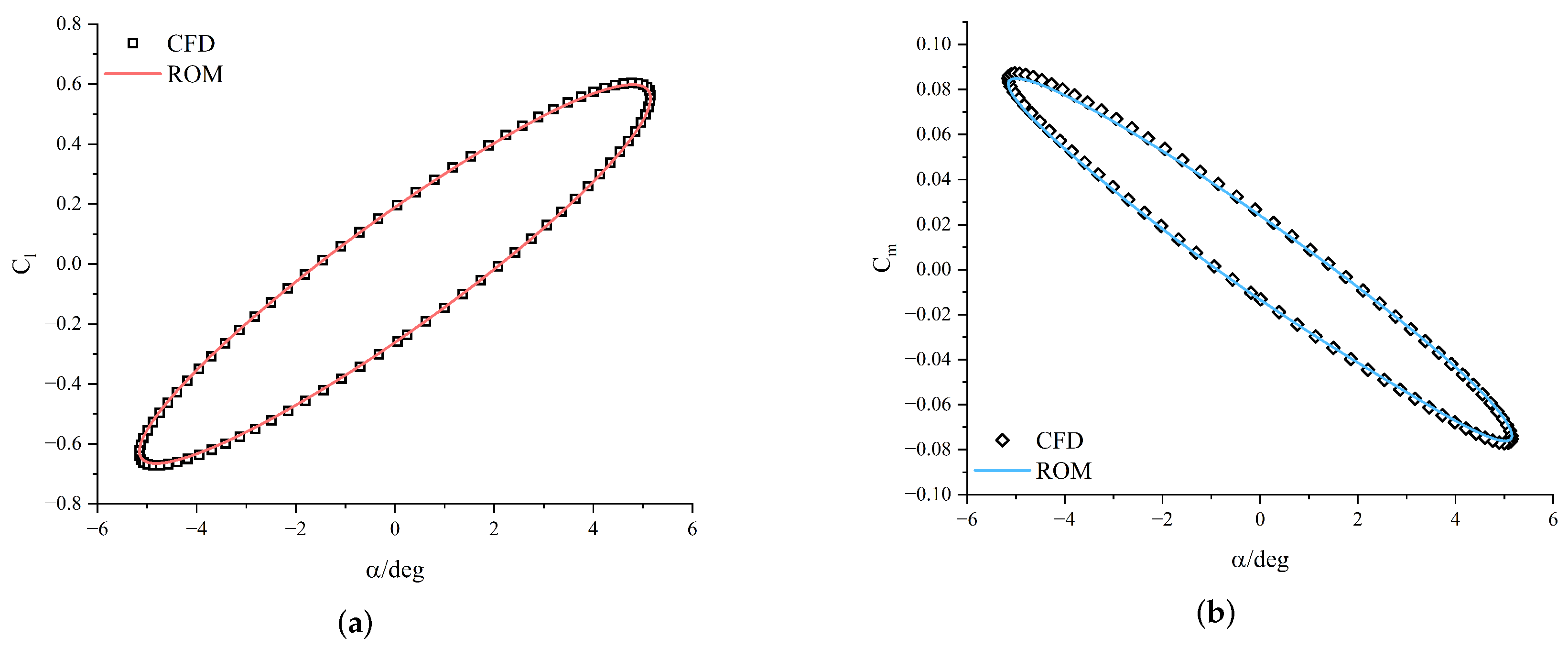
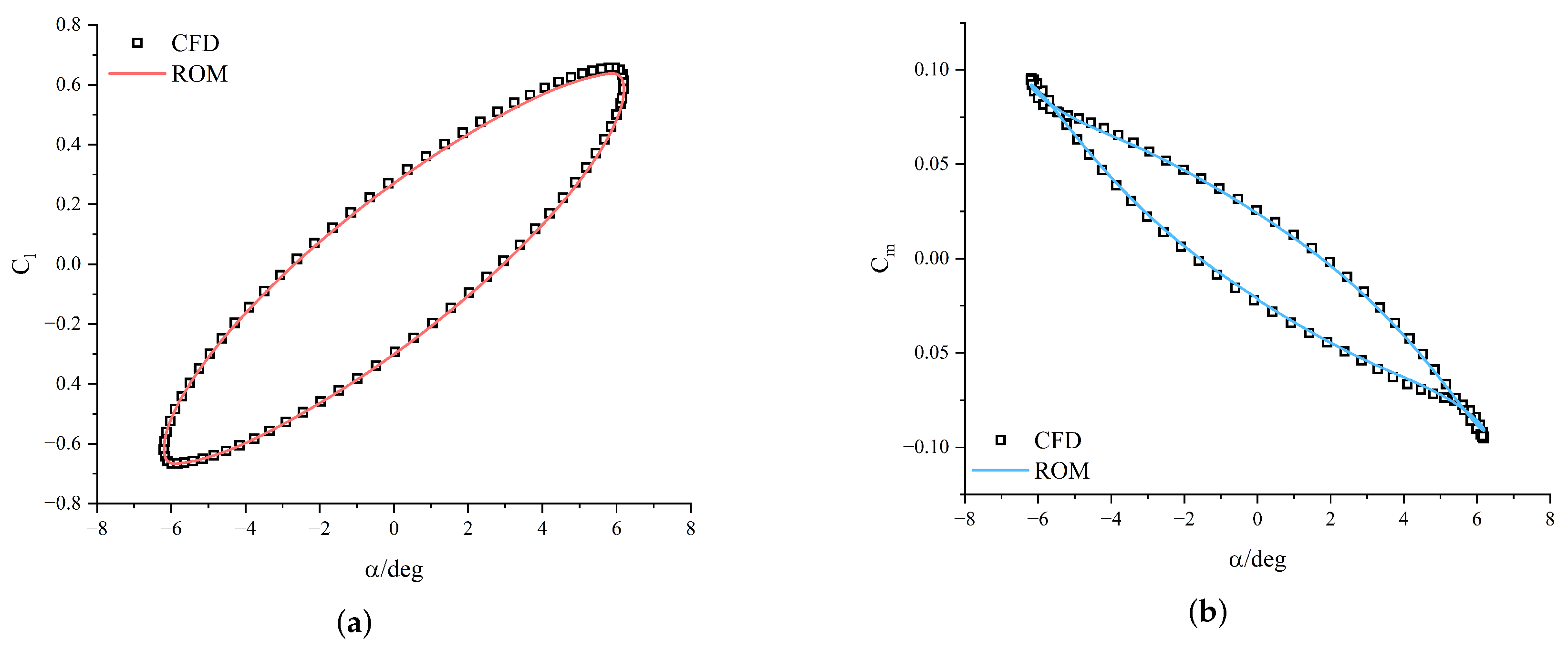
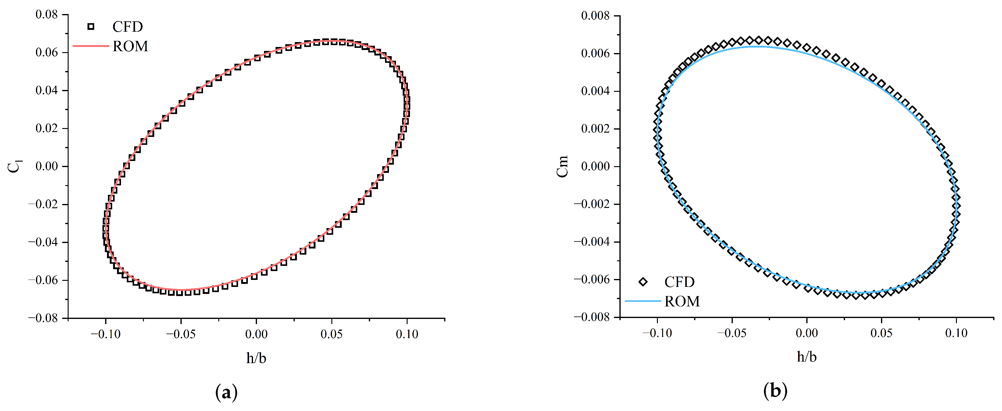
4.2. Prediction of Unsteady Aerodynamics

In this subsection, we primarily introduce the application of the proposed KAN-based reduced-order model for predicting nonlinear unsteady aerodynamic forces. To validate the effectiveness and accuracy of the proposed ROM in capturing complex unsteady aerodynamic behaviors, we applied it to predict the aerodynamic coefficients of an NACA 64A010 airfoil undergoing single-degree-of-freedom forced pitching and plunging harmonic motions. The airfoil motions were centered at the 0.2 chord position, operating at a Mach number of 0.8, which is characterized by the formation of strong shock waves on the airfoil surface. The goal was to assess the ROM’s capability in accurately capturing the nonlinear aerodynamic characteristics across various amplitudes and reduced frequencies k. Predicted aerodynamic coefficients from the KAN-based ROM were compared against high-fidelity CFD simulations to quantitatively evaluate the accuracy and reliability of the proposed approach.

Figure 9, Figure 10 and Figure 11 present predictions of aerodynamic coefficients for the airfoil undergoing single-degree-of-freedom harmonic pitching motions. Similarly, Figure 12, Figure 13 and Figure 14 illustrate predictions for harmonic plunging motions. These figures notably highlight the hysteresis loops of the lift and moment coefficients, demonstrating the model’s ability to accurately replicate the complex unsteady aerodynamic phenomena. The relative error (RE) between the predicted ROM results and CFD simulation data was quantified using the formula provided in Equation (14). A comprehensive summary of test case parameters, along with calculated relative errors for each scenario, is presented in

Table 1. Details of the test cases and the relative error values of the predicted aerodynamic coefficients.

Case	${\mathit{\alpha }}_{\mathit{max}}$	${(\mathit{h}/\mathit{b})}_{\mathit{max}}$	k	$\mathit{RE}\left({\mathit{C}}_{\mathit{l}}\right)$	$\mathit{RE}\left({\mathit{C}}_{\mathit{m}}\right)$
Pitching motion
1	2.865°	0	0.124	1.59%	6.13%
2	5.517°	0	0.089	0.94%	2.25%
3	6.198°	0	0.161	2.60%	4.64%
Plunging motion
4	0°	0.1	0.081	2.26%	4.02%
5	0°	0.34	0.182	1.98%	8.15%
6	0°	0.42	0.154	1.54%	5.62%

. The results consistently demonstrate that the proposed KAN-based ROM achieves high precision across both pitching and plunging motions for various amplitudes and reduced frequencies, aligning closely with the high-fidelity CFD results.

$$RE={\displaystyle \frac{\parallel y_{\mathrm{ROM}}-y_{\mathrm{CFD}}{\parallel }_F}{\parallel y_{\mathrm{CFD}}{\parallel }_F}}\times 100\%$$

(14)

In particular, lift coefficient predictions exhibit consistently minimal deviations, underscoring the robustness of the proposed ROM in capturing the aerodynamic lift accurately. However, the prediction accuracy for the moment coefficient, which is more sensitive to nonlinear aerodynamic effects, is comparatively lower than that of the lift coefficient. This observation further supports the notion that the moment coefficient inherently presents greater challenges for accurate prediction due to its pronounced nonlinear behavior.

It is important to note that the accuracy of the moment coefficient prediction for case 5 in this study is notably lower. Given the data-driven nature of the proposed ROM, its performance is intrinsically linked to the quality and representativeness of the input training data [40]. Consequently, even KAN-based models may encounter limitations in certain complex scenarios. Therefore, the reduced accuracy observed in this case likely stems from the model’s inability to sufficiently extract necessary information from the provided input data. Nonetheless, the overall performance of the KAN-based ROM remains reliable, demonstrating a high degree of precision in predicting nonlinear unsteady aerodynamic forces.

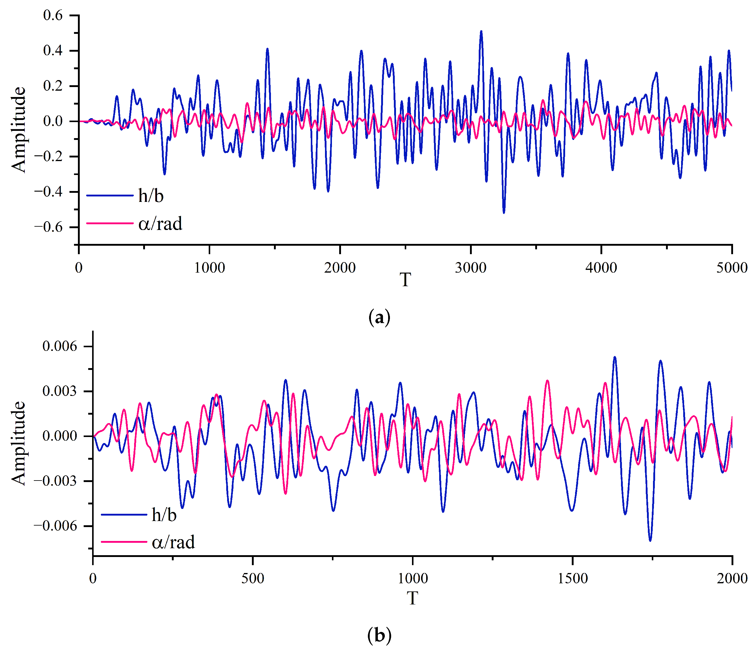
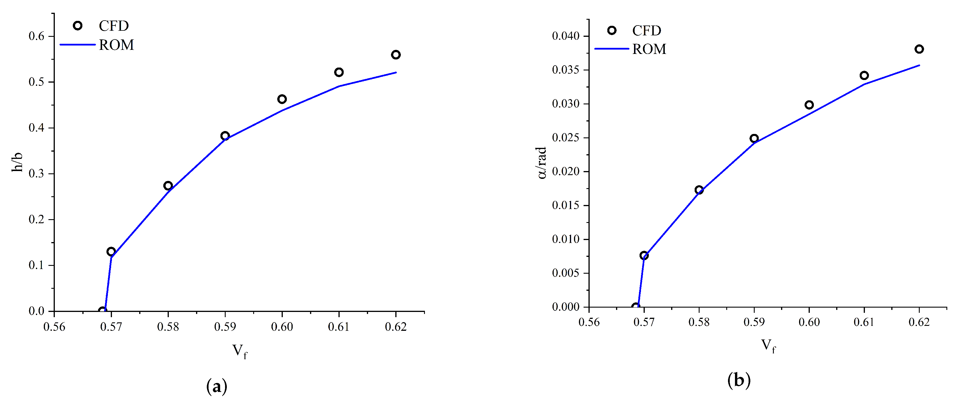
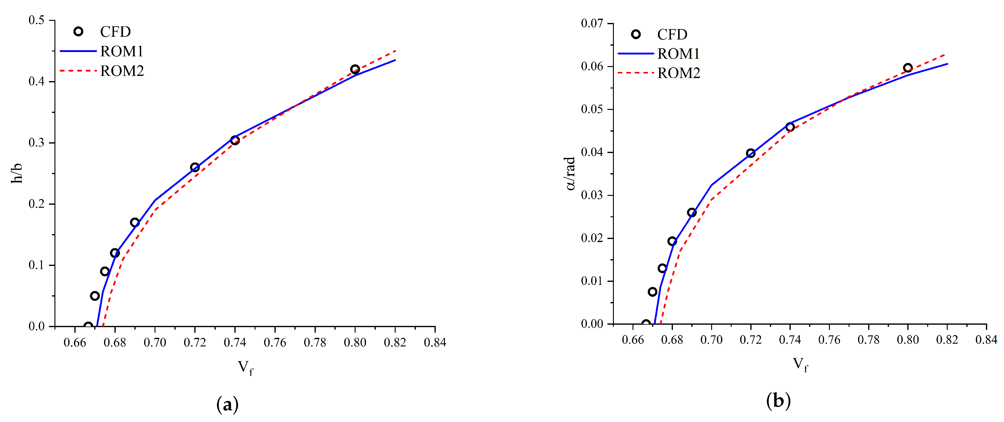
4.3. Prediction of Limit Cycle Oscillations

In this subsection, the nonlinear aerodynamic reduced-order model is coupled with the structural equations of motion to analyze the aeroelastic system. To rigorously assess the predictive capability and precision of the proposed ROM in forecasting limit cycle oscillations (LCO), standard benchmark parameters commonly used in aeroelastic studies [41] are adopted. Specifically, the following parameters are used: the NACA64A010 airfoil, $Ma=0.8$, ${\alpha }_0=0^{\circ }$, $a=-0.6$, $x_{\alpha }=0.25$, $r_{\alpha }^2=0.75$, ${\omega }_h/{\omega }_{\alpha }=0.5$, and $\mu =75$. The use of these established aeroelastic parameters ensures the ROM is tested under physically meaningful and widely recognized conditions, thus demonstrating its suitability and reliability for predicting nonlinear aeroelastic phenomena.

Figure 15 and Figure 16 present a detailed comparison of the limit cycle oscillation responses predicted by the proposed nonlinear ROM and those obtained from high-fidelity CFD simulations at $V_f=0.74$ and $V_f=0.8$, respectively. The results demonstrate that the ROM successfully reproduces the amplitude and waveform of the LCO with high fidelity, highlighting its effectiveness in predicting essential nonlinear aeroelastic behavior. In particular, the ROM exhibits excellent agreement with the initial oscillatory response. However, a gradual phase shift becomes apparent as time progresses. This accumulation of phase discrepancy is primarily attributed to slight differences in the dominant oscillation frequency predicted by the ROM relative to the CFD results. Although these frequency deviations are minimal, they tend to accumulate over time, resulting in a visible phase shift after several oscillation cycles. Such behavior is commonly observed in reduced-order models and reflects the challenges in precisely matching long-term temporal dynamics in nonlinear systems.

Figure 17 further illustrates the comparison of LCO trends across varying flutter speeds, as predicted by the ROM and computed via CFD. The ROM captures the overall trend in LCO amplitude with impressive accuracy, and the predicted results are in close agreement with the CFD data over the entire range. Subsequently, we extend the proposed ROM to the prediction of three-dimensional aeroelastic responses. For validation, the benchmark Active Controls Technology (BACT) model [42] is employed, characterized by an NACA0012 airfoil with parameters ${\alpha }_0=0^{\circ }$, $a=0$, $x_{\alpha }=0.00350$, $r_{\alpha }^2=1.036$, and ${\omega }_h/{\omega }_{\alpha }=0.6539$. Following the same training strategy as in the two-dimensional case, the ROM is applied to predict the three-dimensional aeroelastic responses, and its results are evaluated against CFD simulations. Figure 18 presents a comparison of the LCO trends predicted by the ROM and those obtained from CFD over a range of flutter speeds. The results indicate that the ROM predictions exhibit close agreement with the CFD solutions, highlighting the model’s ability to generalize effectively to three-dimensional aeroelastic response prediction.

In summary, the KAN-based ROM demonstrates strong predictive capabilities for limit cycle oscillations, providing results that are in close agreement with those of direct CFD simulations. This underscores the capability of the proposed data-driven framework to reliably predict nonlinear aeroelastic responses, demonstrating its potential for broader applications in nonlinear dynamical systems.

4.4. Comparison of Time Cost and Model Performance

To further evaluate the performance of the proposed KAN-based ROM, this section presents a comprehensive comparison with the DNN-based ROM proposed by Li et al. [24]. In this subsection, ROM1 refers to the proposed KAN-based reduced-order model, while ROM2 denotes the DNN-based reduced-order model. Both models utilize identical input signals and maintain exactly the same architectural configurations, including the number of layers and units per layer. Under these conditions, ROM1 comprises a total of 10,032 parameters, while ROM2 comprises 12,866 parameters. This represents an approximately 22.0% reduction in the total parameter count. Furthermore, due to its fewer parameters and inherently efficient network structure, ROM1 exhibits superior resistance to overfitting during training, thus achieving enhanced generalization performance.

Table 2. Comparison of relative error values between different ROMs and CFD simulations.

${\mathit{\alpha }}_{max}$	${(\mathit{h}/\mathit{b})}_{max}$	k	Relative Error (ROM1/ROM2)
			$\mathit{RE}\left({\mathit{C}}_{\mathit{l}}\right)$	$\mathit{RE}\left({\mathit{C}}_{\mathit{m}}\right)$
Pitching motion
4.021°	0	0.058	1.89%/1.94%	3.96%/4.88%
5.157°	0	0.119	1.31%/2.21%	4.02%/5.15%
5.749°	0	0.091	1.64%/2.55%	7.15%/6.17%
Plunging motion
0°	0.09	0.166	1.75%/1.60%	4.24%/5.75%
0°	0.15	0.063	0.92%/2.79%	3.96%/6.82%
0°	0.21	0.107	2.01%/1.77%	6.51%/4.64%

compares the relative prediction errors of the two different ROMs with the direct CFD results for unsteady aerodynamic predictions. Figure 19 further illustrates a comparative analysis between the two ROMs’ predictions of the limit cycle oscillations and the corresponding direct CFD computations. The results demonstrate that the proposed ROM1 achieves higher overall prediction accuracy compared to ROM2 in predicting both unsteady aerodynamic and LCO behaviors.

The proposed reduced-order model demonstrates substantial computational efficiency compared to high-fidelity CFD simulations. In the present study, the most computationally intensive step involves the generation of datasets for model training and validation. Specifically, producing 7000 time steps, each encompassing 40 sub-iterations, requires approximately 9 h using 10 CPUs. Furthermore, an additional computational expense emerges during the model training phase, which typically takes around 4 h. However, once trained, the ROM significantly accelerates the prediction of unsteady aerodynamics and LCO responses. Specifically, predicting the unsteady aerodynamic of a single harmonic motion scenario takes approximately 0.7 s with the ROM, a stark contrast to the roughly 1 h required by equivalent CFD simulations. In predicting LCO responses, the ROM completes a prediction in approximately 120 s, while the corresponding high-fidelity CFD computations require approximately 8 h.

These results clearly illustrate the high accuracy and efficiency of the proposed ROM in predicting unsteady aerodynamic and LCO responses. As the number of test scenarios increases, the computational advantage offered by the ROM becomes even more pronounced. Therefore, this approach is particularly beneficial in scenarios where computational resources are limited and rapid analysis turnaround is essential, underscoring the model’s potential in streamlining unsteady aerodynamics and aeroelastic analyses.

5. Conclusions

In this paper, we propose a reduced-order model for unsteady aerodynamics and aeroelasticity based on Kolmogorov–Arnold Networks. Kolmogorov–Arnold Networks are well suited for accurately capturing complex, nonlinear relationships in data, which allows for highly accurate predictions and models across various applications. To capture the time-delay effects, we incorporate a recurrent structure and a gating mechanism, which enable the model to selectively control and preserve long-term temporal dependencies. This design effectively facilitates the modeling of unsteady aerodynamics and aeroelastic responses. The main conclusions are as follows:

(1)

The ROM can accurately predict nonlinear unsteady aerodynamic coefficients under different amplitudes and reduced frequencies.

(2)

The ROM can accurately predict the limit cycle oscillation responses and trends under different flutter speeds.

(3)

The computational efficiency significantly improved compared to direct CFD computations, and the ROM exhibited better generalization than the previous model. These advantages underscore its potential to reduce computational costs while maintaining high fidelity, making it a promising approach for aerodynamic and aeroelastic analysis.

In the future, we aim to further develop and refine Kolmogorov–Arnold Network-based models for broader application to complex aerodynamic and aeroelastic phenomena, such as stall flutter, three-dimensional aeroelastic problems, and transonic buffet. The goal is to enhance both predictive accuracy and computational efficiency, thereby extending the practical application of these models across a wider range of scenarios.

References

- Zhou, Q.; Li, D.F.; Da Ronch, A.; Chen, G.; Li, Y.M. Computational fluid dynamics-based transonic flutter suppression with control delay. J. Fluids Struct. 2016, 66, 183–206. [Google Scholar] [CrossRef]
- Chen, P.C.; Zhang, Z.; Livne, E. Design-oriented computational fluid dynamics-based unsteady aerodynamics for flight-vehicle aeroelastic shape optimization. AIAA J. 2015, 53, 3603–3619. [Google Scholar] [CrossRef]
- Farhat, C.; Lesoinne, M. Two efficient staggered algorithms for the serial and parallel solution of three-dimensional nonlinear transient aeroelastic problems. Comput. Methods Appl. Mech. Eng. 2000, 182, 499–515. [Google Scholar] [CrossRef]
- Bendiksen, O.O. Transonic limit cycle flutter of high-aspect-ratio swept wings. J. Aircr. 2008, 45, 1522–1533. [Google Scholar] [CrossRef]
- Wei, L.; Zheng, G.; Nie, X.; Lv, J.; Huang, C.; Lu, W.; Zhang, Y.; Yang, G. Robustness and Efficiency of Encapsulated Selective Frequency Damping Using Different Operator-Splitting Schemes: Application to Laminar Cylinder Flow and Transonic Buffet. J. Comput. Phys. 2025, 532, 113968. [Google Scholar] [CrossRef]
- Dean, J.; Morton, S.; McDaniel, D.; Clifton, J.; Bodkin, D. Aircraft stability and control characteristics determined by system identification of CFD simulations. In Proceedings of the AIAA Atmospheric Flight Mechanics Conference and Exhibit, Honolulu, HI, USA, 18–21 August 2008; p. 6378. [Google Scholar]
- Ghoreyshi, M.; Jirásek, A.; Cummings, R.M. Reduced order unsteady aerodynamic modeling for stability and control analysis using computational fluid dynamics. Prog. Aerosp. Sci. 2014, 71, 167–217. [Google Scholar] [CrossRef]
- Zhang, W.; Ye, Z. Reduced-order-model-based flutter analysis at high angle of attack. J. Aircr. 2007, 44, 2086–2089. [Google Scholar] [CrossRef]
- Cowan, T.J.; Arena, A.S., Jr.; Gupta, K.K. Accelerating computational fluid dynamics based aeroelastic predictions using system identification. J. Aircr. 2001, 38, 81–87. [Google Scholar] [CrossRef]
- Roy, A.; Mukherjee, R. Time Series Behaviour of Laminar Separation Bubbles at Low Reynolds Number. In Proceedings of the AIAA Scitech 2021 Forum, Virtual, 11–15, 19–21 January 2021; p. 1197. [Google Scholar]
- Huang, R.; Hu, H.; Zhao, Y. Nonlinear reduced-order modeling for multiple-input/multiple-output aerodynamic systems. AIAA J. 2014, 52, 1219–1231. [Google Scholar] [CrossRef]
- Cheng, C.M.; Peng, Z.K.; Zhang, W.M.; Meng, G. Volterra-series-based nonlinear system modeling and its engineering applications: A state-of-the-art review. Mech. Syst. Signal Process. 2017, 87, 340–364. [Google Scholar] [CrossRef]
- Lee, B.H.K. Oscillatory shock motion caused by transonic shock boundary-layer interaction. AIAA J. 1990, 28, 942–944. [Google Scholar] [CrossRef]
- Lee, B.H.K. Self-sustained shock oscillations on airfoils at transonic speeds. Prog. Aerosp. Sci. 2001, 37, 147–196. [Google Scholar] [CrossRef]
- Hermes, V.; Klioutchnikov, I.; Olivier, H. Numerical investigation of unsteady wave phenomena for transonic airfoil flow. Aerosp. Sci. Technol. 2013, 25, 224–233. [Google Scholar] [CrossRef]
- Brunton, S.L.; Noack, B.R.; Koumoutsakos, P. Machine learning for fluid mechanics. Annu. Rev. Fluid Mech. 2020, 52, 477–508. [Google Scholar] [CrossRef]
- Liu, Y.; Wang, F.; Zhao, S.; Tang, Y. A novel framework for predicting active flow control by combining deep reinforcement learning and masked deep neural network. Phys. Fluids 2024, 36, 037112. [Google Scholar] [CrossRef]
- Kou, J.; Zhang, W. Data-driven modeling for unsteady aerodynamics and aeroelasticity. Prog. Aerosp. Sci. 2021, 125, 100725. [Google Scholar] [CrossRef]
- Zhang, W.; Wang, B.; Ye, Z.; Quan, J. Efficient method for limit cycle flutter analysis based on nonlinear aerodynamic reduced-order models. AIAA J. 2012, 50, 1019–1028. [Google Scholar] [CrossRef]
- Zhang, W.; Kou, J.; Wang, Z. Nonlinear aerodynamic reduced-order model for limit-cycle oscillation and flutter. AIAA J. 2016, 54, 3304–3311. [Google Scholar] [CrossRef]
- Winter, M.; Breitsamter, C. Neurofuzzy-model-based unsteady aerodynamic computations across varying freestream conditions. AIAA J. 2016, 54, 2705–2720. [Google Scholar] [CrossRef]
- Winter, M.; Breitsamter, C. Nonlinear identification via connected neural networks for unsteady aerodynamic analysis. Aerosp. Sci. Technol. 2018, 77, 802–818. [Google Scholar] [CrossRef]
- Qi, H.; Yu, J.; Jiang, J.; Guo, J. Linear and nonlinear combined aerodynamic reduced order model based on residual network framework. Europhys. Lett. 2022, 138, 63002. [Google Scholar] [CrossRef]
- Li, K.; Kou, J.; Zhang, W. Deep neural network for unsteady aerodynamic and aeroelastic modeling across multiple Mach numbers. Nonlinear Dyn. 2019, 96, 2157–2177. [Google Scholar] [CrossRef]
- Dai, Y.; Rong, H.; Wu, Y.; Yang, C.; Xu, Y. Stall flutter prediction based on multi-layer GRU neural network. Chin. J. Aeronaut. 2023, 36, 75–90. [Google Scholar] [CrossRef]
- Liu, Z.; Wang, Y.; Vaidya, S.; Ruehle, F.; Halverson, J.; Soljačić, M.; Hou, T.; Tegmark, M. Kan: Kolmogorov-arnold networks. arXiv 2024, arXiv:2404.19756. [Google Scholar]
- Liu, Z.; Ma, P.; Wang, Y.; Matusik, W.; Tegmark, M. Kan 2.0: Kolmogorov-arnold networks meet science. arXiv 2024, arXiv:2408.10205. [Google Scholar]
- Ji, T.; Hou, Y.; Zhang, D. A comprehensive survey on Kolmogorov Arnold networks (KAN). arXiv 2024, arXiv:2407.11075. [Google Scholar]
- Polo-Molina, A.; Alfaya, D.; Portela, J. MonoKAN: Certified Monotonic Kolmogorov-Arnold Network. arXiv 2024, arXiv:2409.11078. [Google Scholar]
- Koenig, B.C.; Kim, S.; Deng, S. KAN-ODEs: Kolmogorov–Arnold network ordinary differential equations for learning dynamical systems and hidden physics. Comput. Methods Appl. Mech. Eng. 2024, 432, 117397. [Google Scholar] [CrossRef]
- Aghaei, A.A. KANtrol: A Physics-Informed Kolmogorov-Arnold Network Framework for Solving Multi-Dimensional and Fractional Optimal Control Problems. arXiv 2024, arXiv:2409.06649. [Google Scholar]
- Genet, R.; Inzirillo, H. Tkan: Temporal kolmogorov-arnold networks. arXiv 2024, arXiv:2405.07344. [Google Scholar] [CrossRef]
- Xu, K.; Chen, L.; Wang, S. Kolmogorov-arnold networks for time series: Bridging predictive power and interpretability. arXiv 2024, arXiv:2406.02496. [Google Scholar]
- Zhou, Q.; Pei, C.; Sun, F.; Han, J.; Gao, Z.; Pei, D.; Zhang, H.; Xie, G.; Li, J. KAN-AD: Time series anomaly detection with Kolmogorov-Arnold networks. arXiv 2024, arXiv:2411.00278. [Google Scholar]
- Tan, Y. Numerical Analysis and Suppression of Transonic Airfoil Flutter. Master’s Thesis, University of Chinese Academy of Sciences, Beijing, China, 2023. [Google Scholar]
- Landon, R.H. NACA 0012 oscillatory and transient pitching. AGARD Rep. 1982, 702, 45–59. [Google Scholar]
- Isogai, K. On the transonic-dip mechanism of flutter of a sweptback wing. AIAA J. 1979, 17, 793–795. [Google Scholar] [CrossRef]
- Hota, H.S.; Handa, R.; Shrivas, A.K. Time series data prediction using sliding window based RBF neural network. Int. J. Comput. Intell. Res. 2017, 13, 1145–1156. [Google Scholar]
- Halder, R.; Damodaran, M.; Khoo, B.C. Deep learning based reduced order model for airfoil-gust and aeroelastic interaction. AIAA J. 2020, 58, 4304–4321. [Google Scholar] [CrossRef]
- Brewick, P.T.; Masri, S.F. An evaluation of data-driven identification strategies for complex nonlinear dynamic systems. Nonlinear Dyn. 2016, 85, 1297–1318. [Google Scholar] [CrossRef]
- Thomas, J.P.; Dowell, E.H.; Hall, K.C. Nonlinear inviscid aerodynamic effects on transonic divergence, flutter, and limit-cycle oscillations. AIAA J. 2002, 40, 638–646. [Google Scholar] [CrossRef]
- Rivera, J., Jr.; Dansberry, B.; Bennett, R.; Durham, M.; Silva, A.W. NACA 0012 benchmark model experimental flutter results with unsteady pressure distributions. In Proceedings of the 33rd Structures, Structural Dynamics and Materials Conference, Dallas, TX, USA, 13–15 April 1992; p. 2396. [Google Scholar]