Real-Time Intelligent Recognition and Precise Drilling in Strongly Heterogeneous Formations Based on Multi-Parameter Logging While Drilling and Drilling Engineering

 , and
, and 
Abstract
1. Introduction
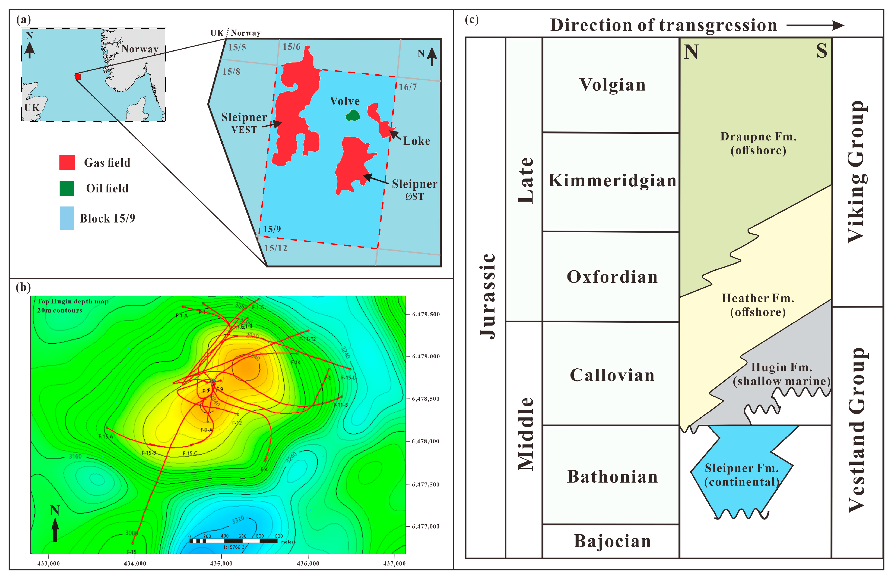
2. Study Area and Data
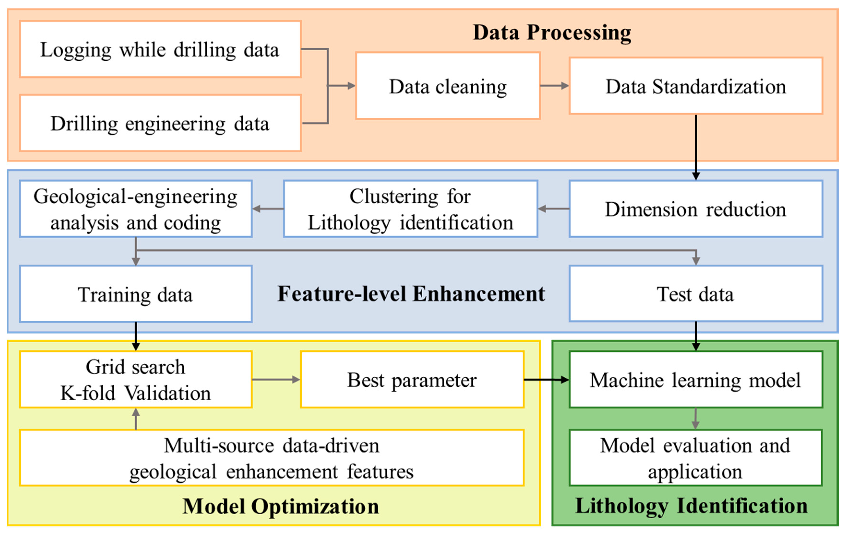
3. Methodology
3.1. Data Preprocessing Methods
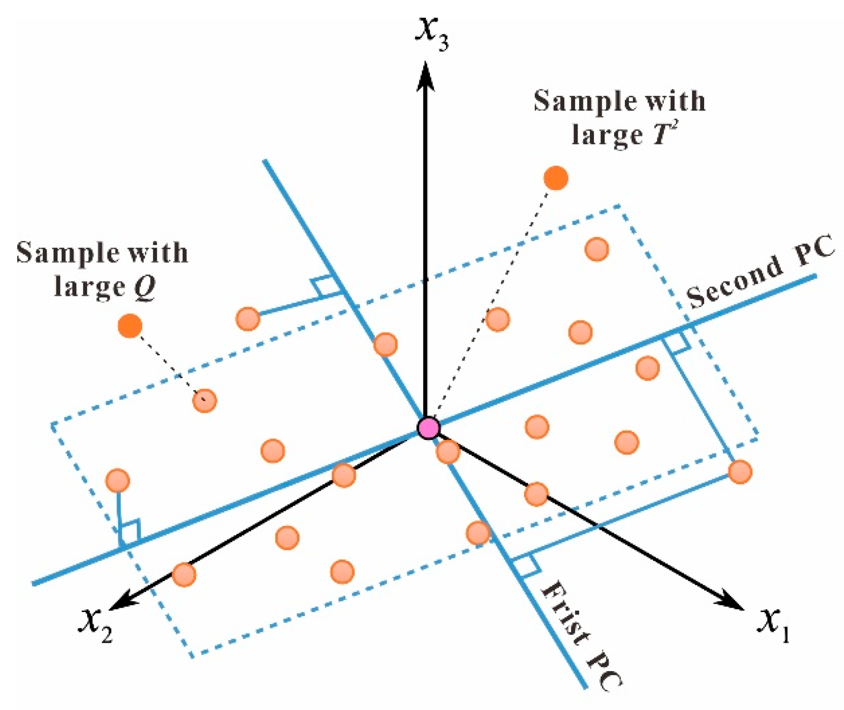
3.2. Dimensionality Reduction Algorithm
- (1)
- PCA
- (2)
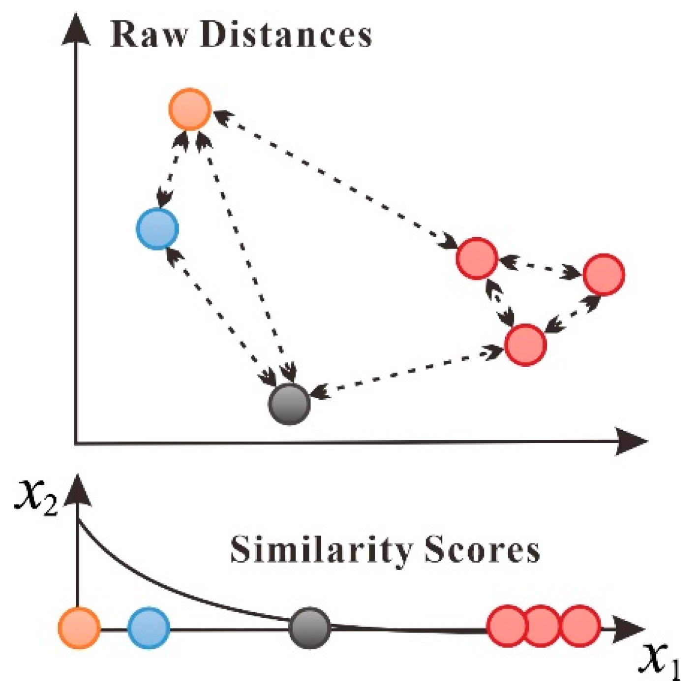
- t-SNE
- (3)
- UMAP
3.3. Intelligent Recognition Algorithm
- (1)
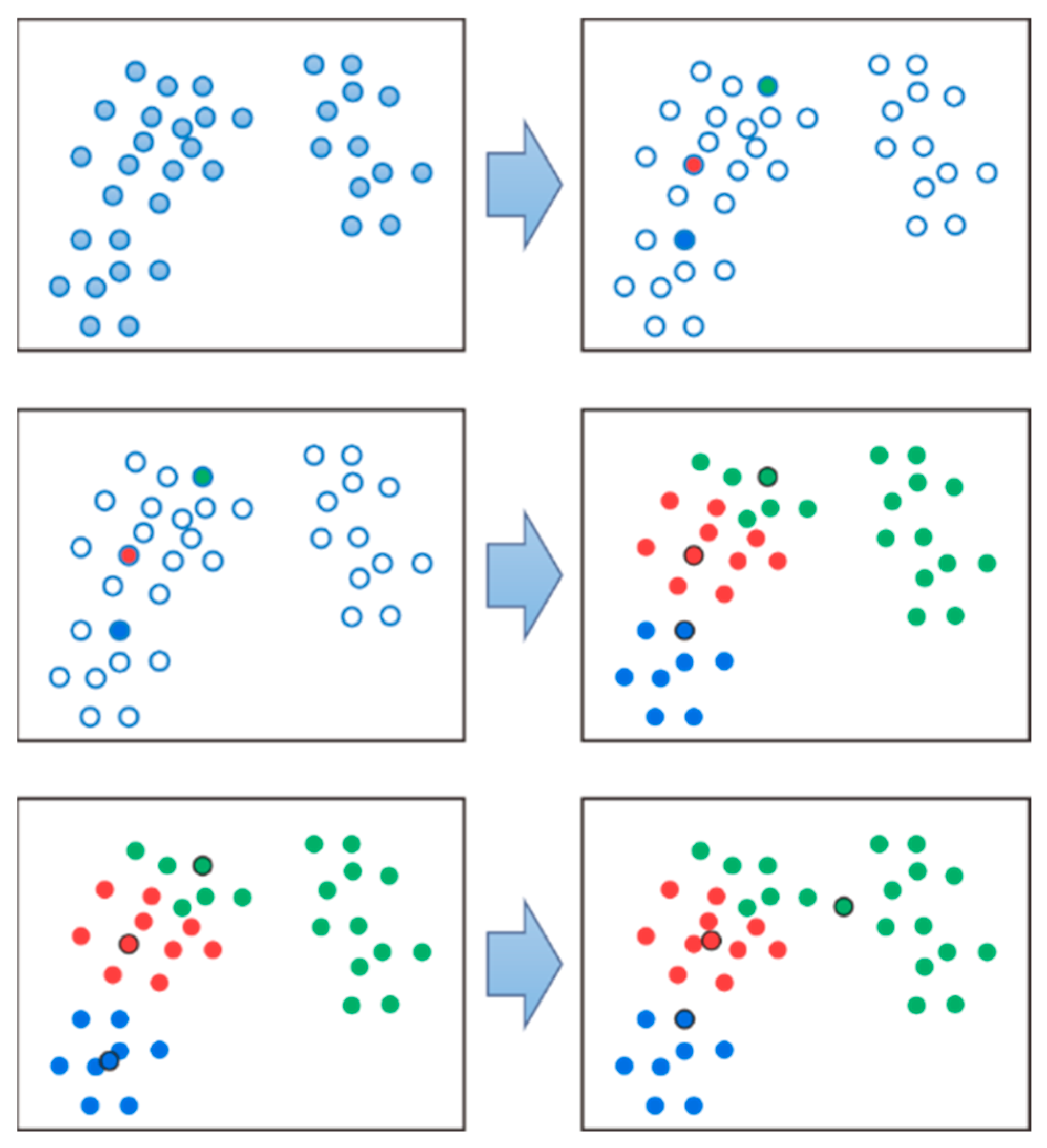
- K-means
- (2)
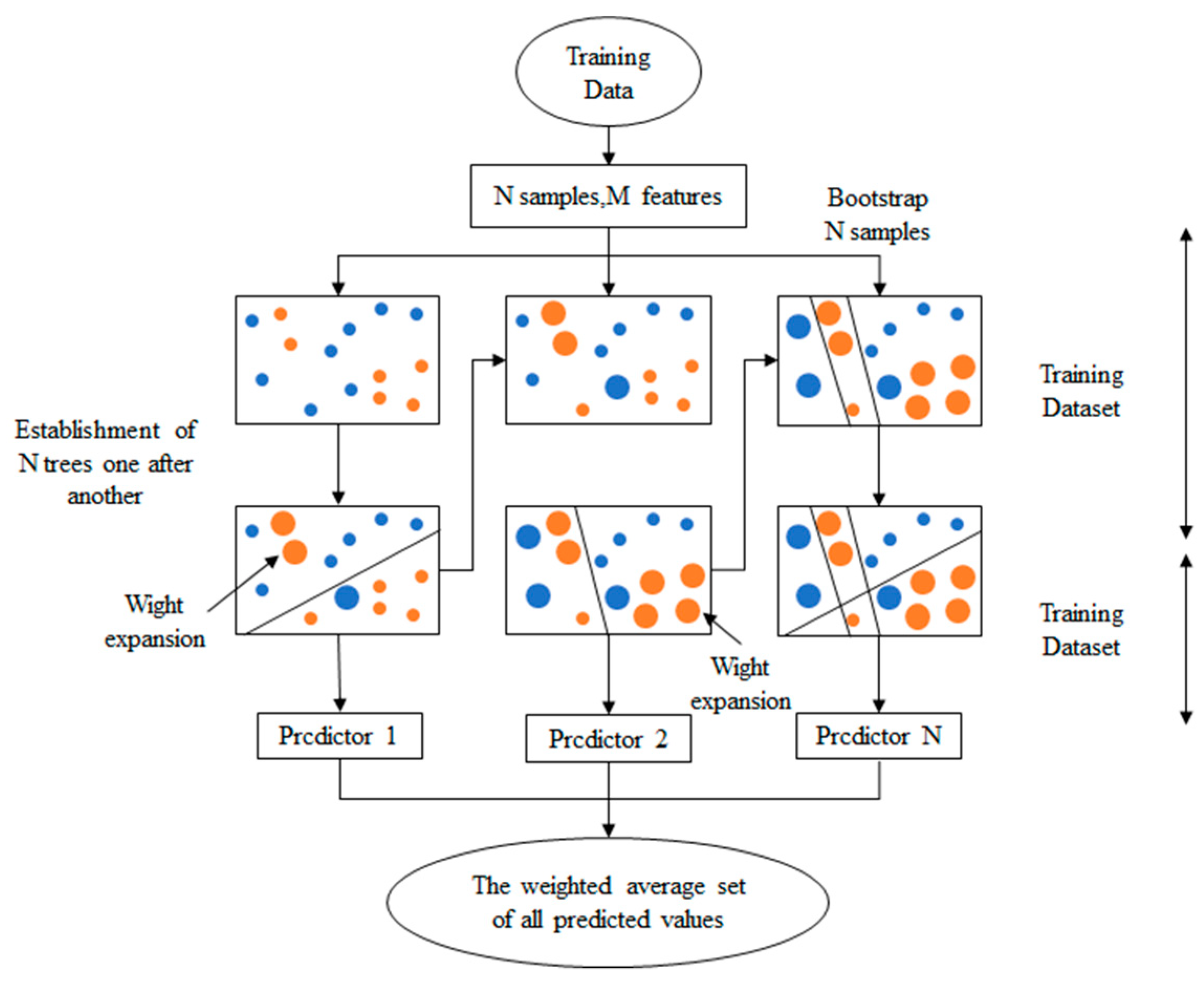
- CatBoost
3.4. Model Evaluation System
- (1)
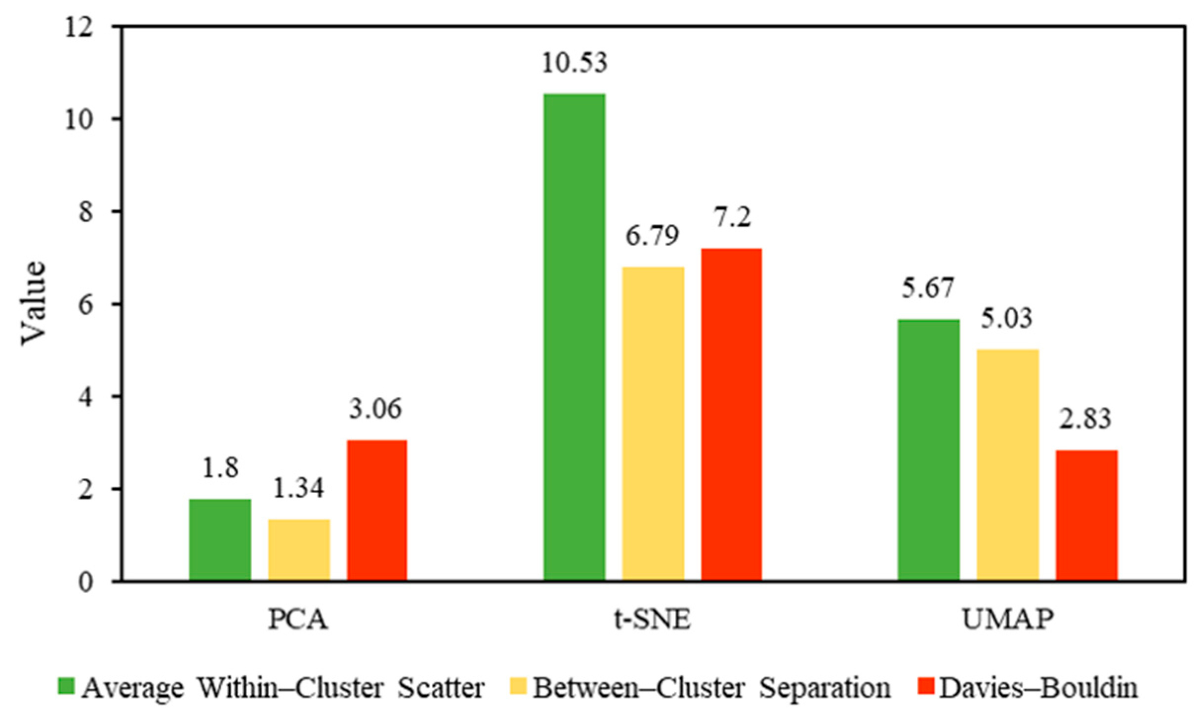
- Clustering evaluation index
- (2)
- Recognition model evaluation index
4. Results
4.1. Dataset Description
4.2. Data Preprocessing
4.3. Lithology Classification Feature Extraction
- (1)
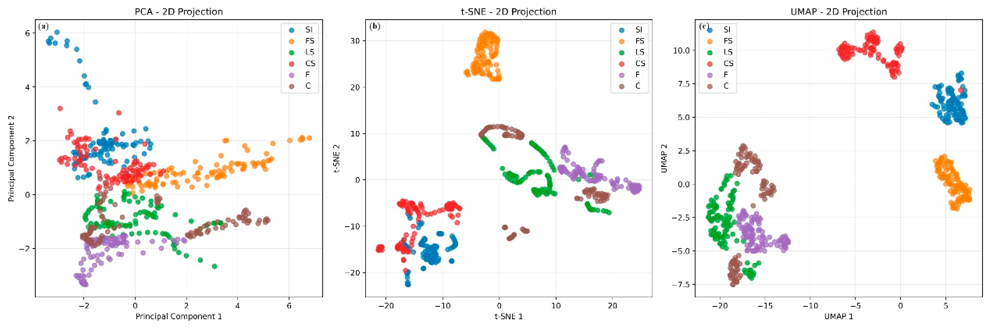
- Dimension reduction
- (2)
- Cluster processing
4.4. Application of Lithology Identification Model
- (1)
- Model training
- (2)
- Model testing
5. Discussion
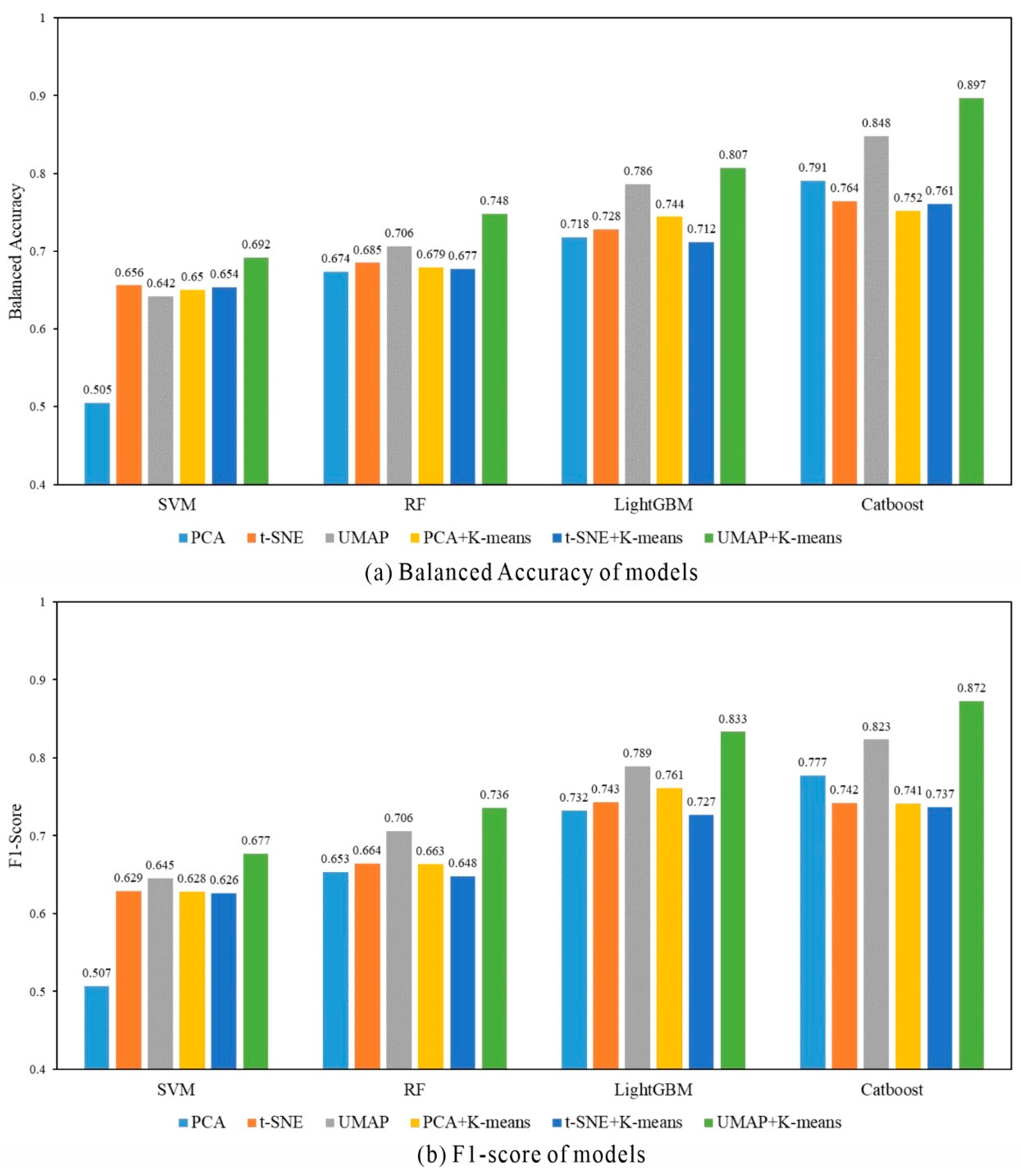
5.1. Comparing the Performances of Different Machine Learning Algorithms
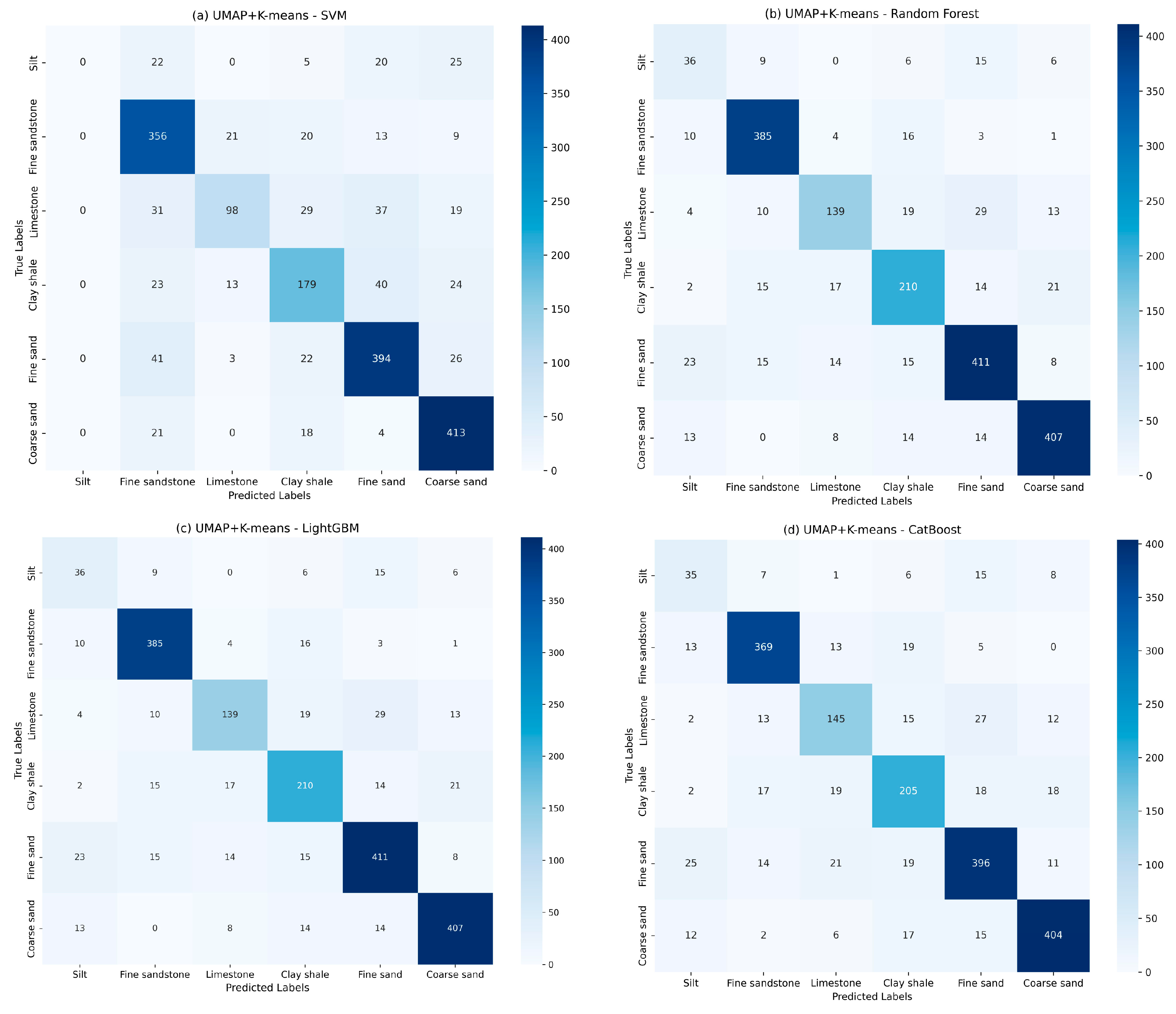
5.2. Performance Analysis of the Optimal Method for Identifying Highly Heterogeneous Formations
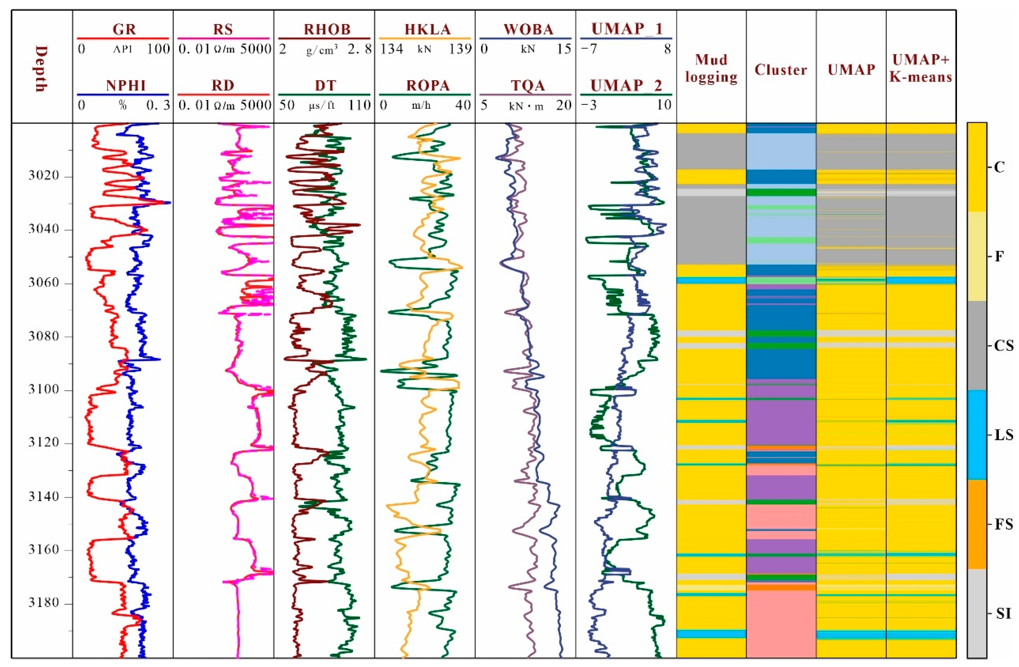
5.3. Real-Time Optimization of Drilling Parameters Based on Strongly Heterogeneous Formation Identification
5.4. Model Generalizability and Adaptation Strategies
6. Conclusions
Author Contributions
Funding
Institutional Review Board Statement
Informed Consent Statement
Data Availability Statement
Acknowledgments
Conflicts of Interest
Abbreviations
| PCA | Principal Component Analysis |
| t-SNE | t-Distributed Stochastic Neighbor Embedding |
| UMAP | Uniform Manifold Approximation and Projection |
| DBI | Davies–Bouldin Index |
| SVM | Support Vector Machine |
| RF | Random Forest |
| LightGBM | Lightweight Gradient Boosting Machine |
| CatBoost | Categorical Boosting |
References
- Li, G.S.; Song, X.Z.; Zhu, Z.P.; Tian, S.Z.; Sheng, M. Research progress and the prospect of intelligent drilling and completion technologies. Pet. Drill. Tech. 2023, 51, 35–47. [Google Scholar] [CrossRef]
- Xiong, Q.P.; Cheng, Z.J.; Wen, Y.W. Petroleum geology features and research developments of hydrocarbon accumulation in deep petroliferous basins. Pet. Sci. 2015, 12, 1–53. [Google Scholar] [CrossRef]
- Sun, L.D.; Zou, C.N.; Jia, A.L.; Wei, Y.S.; Zhu, R.K.; Wu, S.T.; Guo, Z. Development characteristics and orientation of tight oil and gas in China. Pet. Explor. Dev. 2019, 46, 1073–1087. [Google Scholar] [CrossRef]
- Holenka, J.; Best, D.; Evans, M.; Kurkoski, P.; Sloan, W. Azimuthal porosity while drilling. In Proceedings of the SPWLA Annual Logging Symposium, Paris, France, 12–15 June 1995; p. SPWLA-1995-BB. [Google Scholar]
- Bornemann, E.; Bourgeois, T.; Bramlett, K.; Hodenfield, K.; Maggs, D. The application and accuracy of geological information from a logging-while-drilling density tool. In Proceedings of the SPWLA Annual Logging Symposium, Keystone, CO, USA, 26–29 May 1998; p. SPWLA-1998-L. [Google Scholar]
- Carpenter, W.W.; Best, D.; Evans, M. Applications and interpretation of azimuthally sensitive density measurements acquired while drilling. In Proceedings of the SPWLA Annual Logging Symposium, Houston, TX, USA, 15–18 June 1997; p. SPWLA-1997-EE. [Google Scholar]
- Qin, Z.; Tang, B.; Wu, D.; Luo, S.C.; Ma, X.G.; Huang, K.; Deng, C.X.; Yang, H.J.; Pan, H.P.; Wang, Z.H. A qualitative characteristic scheme and a fast distance prediction method of multi-probe azimuthal gamma-ray logging in geosteering. J. Pet. Sci. Eng. 2021, 199, 108244. [Google Scholar] [CrossRef]
- Tian, F.; Di, Q.Y.; Zheng, W.H.; Ge, X.M.; Zhang, W.X.; Zhang, J.Y.; Yang, C.C. A formation intelligent evaluation solution for geosteering. Chin. J. Geophys. 2023, 66, 3975–3989. [Google Scholar] [CrossRef]
- Datta, D.; Singh, G.; Routray, A.; Mohanty, W.K.; Mahadik, R. Automatic Classification of Lithofacies with Highly Imbalanced Dataset Using Multistage SVM Classifier. In Proceedings of the IECON 2021–47th Annual Conference of the IEEE Industrial Electronics Society, Toronto, ON, Canada, 13–16 October 2021; pp. 1–6. [Google Scholar] [CrossRef]
- Li, Y.P.; Luo, M.L.; Ma, S.X.; Lu, P. Massive Spatial Well Clustering Based on Conventional Well Log Feature Extraction for Fast Formation Heterogeneity Characterization. Lithosphere 2022, 2022, 7260254. [Google Scholar] [CrossRef]
- Martins Saporetti, C.; Da Fonseca, L.G.; Pereira, E.; Costa De Oliveira, L. Machine learning approaches for petrographic classification of carbonate-siliciclastic rocks using well logs and textural information. J. Appl. Geophys. 2018, 155, 217–225. [Google Scholar] [CrossRef]
- Tian, F.; Jin, Q.; Lu, X.B.; Lei, Y.H.; Zhang, L.K.; Zheng, S.Q.; Zhang, H.F.; Rong, Y.S.; Liu, N.G. Multi-layered ordovician paleokarst reservoir detection and spatial delineation: A case study in the Tahe Oilfield, Tarim Basin, Western China. Mar. Pet. Geol. 2016, 69, 53–73. [Google Scholar] [CrossRef]
- Tian, F.; Di, Q.Y.; Jin, Q.; Cheng, F.Q.; Zhang, W.; Lin, L.M.; Wang, Y.; Yang, D.B.; Niu, C.K.; Li, Y.X. Multiscale geological-geophysical characterization of the epigenic origin and deeply buried paleokarst system in Tahe Oilfield, Tarim Basin. Mar. Pet. Geol. 2019, 102, 16–32. [Google Scholar] [CrossRef]
- Tian, F.; Luo, X.R.; Zhang, W. Integrated geological-geophysical characterizations of deeply buried fractured-vuggy carbonate reservoirs in Ordovician strata, Tarim Basin. Mar. Pet. Geol. 2019, 99, 292–309. [Google Scholar] [CrossRef]
- Xing, Y.H.; Yang, H.T.; Yu, W. An Approach for the Classification of Rock Types Using Machine Learning of Core and Log Data. Sustainability 2023, 15, 8868. [Google Scholar] [CrossRef]
- Zhang, J.L.; He, Y.B.; Zhang, Y.; Li, W.F.; Zhang, J.J. Well-Logging-Based Lithology Classification Using Machine Learning Methods for High-Quality Reservoir Identification: A Case Study of Baikouquan Formation in Mahu Area of Junggar Basin, NW China. Energies 2022, 15, 3675. [Google Scholar] [CrossRef]
- Baudzis, S.; Karłowska-Pik, J.; Puskarczyk, E. Electrofacies as a Tool for the Prediction of True Resistivity Using Advanced Statistical Methods—Case Study. Energies 2021, 14, 6228. [Google Scholar] [CrossRef]
- Zheng, W.H.; Tian, F.; Di, Q.Y.; Xin, W.; Cheng, F.Q.; Shan, X.C. Electrofacies classification of deeply buried carbonate strata using machine learning methods: A case study on ordovician paleokarst reservoirs in Tarim Basin. Mar. Pet. Geol. 2021, 123, 104720. [Google Scholar] [CrossRef]
- Liu, J.Y.; Tian, F.; Zhao, A.S.; Zheng, W.H.; Cao, W.J. Logging Lithology Discrimination with Enhanced Sampling Methods for Imbalance Sample Conditions. Appl. Sci. 2024, 14, 6534. [Google Scholar] [CrossRef]
- Mcdonald, W.J.; Ward, C.E. Logging while drilling: A survey of methods and priorities. In Proceedings of the SPWLA Annual Logging Symposium, Denver, CO, USA, 9–12 June 1976; p. SPWLA-1976-U. [Google Scholar]
- De Andreacute, C.A.; Da Cunha, A.M.V.; Boonen, P.; Valant-Spaight, B.; Lefors, S.; Schultz, W. A comparison of logging-while-drilling and wireline nuclear porosity logs in shales from wells in Brazil. Petrophysics 2005, 46, 295–301. [Google Scholar]
- Meador, R.A. Logging while drilling: A Story of Dreams, Accomplishments, And Bright Futures. In Proceedings of the SPWLA Annual Logging Symposium, The Woodlands, TX, USA, 15–19 June 2009; p. SPWLA-2009-43458. [Google Scholar]
- Tollefsen, E.; Weber, A.; Kramer, A.; Sirkin, G.; Hartman, D.; Grant, L. Logging While Drilling Measurements: From Correlation to Evaluation. In Proceedings of the SPE International Oil Conference and Exhibition in Mexico, Veracruz, Mexico, 27 June 2007. [Google Scholar] [CrossRef]
- Neville, T.J.; Weller, G.; Faivre, O.; Sun, H. A new-generation LWD tool with colocated sensors opens new opportunities for formation evaluation. SPE Reserv. Eval. Eng. 2007, 10, 132–139. [Google Scholar] [CrossRef]
- Akinsanmi, O.B.; Aibangbe, O.; Kienitz, C. Application of azimuthal density while drilling images for dips, facies and reservoir characterization—Niger/delta experience. In Proceedings of the SPE/CIM International Conference on Horizontal Well Technology, Calgary, AB, Canada, 6 November 2000; SPE: Calgary, AB, Canada, 2000. [Google Scholar] [CrossRef]
- Ijasan, O.; Torres-Verdín, C.; Preeg, W.E. Inversion-based petrophysical interpretation of logging-while-drilling nuclear and resistivity measurements. Geophysics 2013, 78, D473–D489. [Google Scholar] [CrossRef]
- Landar, S.; Velychkovych, A.; Ropyak, L.; Andrusyak, A. A method for applying the use of a smart 4 controller for the assessment of drill string bottom-part vibrations and shock loads. Vibration 2024, 7, 802–828. [Google Scholar] [CrossRef]
- Velychkovych, A.; Mykhailiuk, V.; Andrusyak, A. Numerical Model for Studying the Properties of a New Friction Damper Developed Based on the Shell with a Helical Cut. Appl. Mech. 2025, 6, 1. [Google Scholar] [CrossRef]
- Velichkovich, A.; Dalyak, T.; Petryk, I. Slotted shell resilient elements for drilling shock absorbers. Oil Gas Sci. Technol.–Rev. D’ifp Energ. Nouv. 2018, 73, 34. [Google Scholar] [CrossRef]
- Vukadin, D.; Čogelja, Z.; Vidaček, R.; Brkić, V. Lithology and Porosity Distribution of High-Porosity Sandstone Reservoir in North Adriatic Using Machine Learning Synthetic Well Catalogue. Appl. Sci. 2023, 13, 7671. [Google Scholar] [CrossRef]
- Ren, Q.; Zhang, H.B.; Zhang, D.L.; Zhao, X.; Yan, L.Z.; Rui, J.W. A novel hybrid method of lithology identification based on k-means++ algorithm and fuzzy decision tree. J. Pet. Sci. Eng. 2022, 208, 109681. [Google Scholar] [CrossRef]
- Zheng, D.; Liu, S.; Chen, Y.; Gu, B. A Lithology Recognition Network Based on Attention and Feature Brownian Distance Covariance. Appl. Sci. 2024, 14, 1501. [Google Scholar] [CrossRef]
- Zhong, R.Z.; Johnson, R.L., Jr.; Chen, Z.W. Using machine learning methods to identify coal pay zones from drilling and logging-while-drilling (LWD) data. SPE J. 2020, 25, 1241–1258. [Google Scholar] [CrossRef]
- Sun, J.; Li, Q.; Chen, M.Q.; Ren, L.; Huang, G.H.; Li, C.Y.; Zhang, Z.X. Optimization of models for a rapid identification of lithology while drilling—A win-win strategy based on machine learning. J. Pet. Sci. Eng. 2019, 176, 321–341. [Google Scholar] [CrossRef]
- Xu, T.; Zhang, W.T.; Li, J.; Liu, H.N.; Kang, Y.; Lv, W.J. Domain generalization using contrastive domain discrepancy optimization for interpretation-while-drilling. J. Nat. Gas Sci. Eng. 2022, 105, 104685. [Google Scholar] [CrossRef]
- Mutrif Siddig, O.; Elkatatny, S. Utilizing Drilling Data and Machine Learning in Real-Time Prediction of Poisson’s Ratio. In Proceedings of the SPE Middle East Oil and Gas Show and Conference, Manama, Bahrain, 19–21 February 2023; p. 021. [Google Scholar] [CrossRef]
- Oloruntobi, O.; Butt, S. Application of specific energy for lithology identification. J. Pet. Sci. Eng. 2020, 184, 106402. [Google Scholar] [CrossRef]
- Mishra, A.; Sharma, A.; Patidar, A.K. Evaluation and Development of a Predictive Model for Geophysical Well Log Data Analysis and Reservoir Characterization: Machine Learning Applications to Lithology Prediction. Nat. Resour. Res. 2022, 31, 3195–3222. [Google Scholar] [CrossRef]
- Smillie, Z.; Demyanov, V.; Mckinley, J.; Cooper, M. Unsupervised classification applications in enhancing lithological mapping and geological understanding: A case study from Northern Ireland. J. Geol. Soc. 2023, 180, jgs2022-136. [Google Scholar] [CrossRef]
- Iraji, S.; Soltanmohammadi, R.; Matheus, G.F.; Basso, M.; Vidal, A.C. Application of unsupervised learning and deep learning for rock type prediction and petrophysical characterization using multi-scale data. Geoenergy Sci. Eng. 2023, 230, 212241. [Google Scholar] [CrossRef]
- Yang, X.; Chen, J.G.; Chen, Z.J. Classification of Alteration Zones Based on Drill Core Hyperspectral Data Using Semi-Supervised Adversarial Autoencoder: A Case Study in Pulang Porphyry Copper Deposit, China. Remote Sens. 2023, 15, 1059. [Google Scholar] [CrossRef]
- Singh, H.; Seol, Y.; Myshakin, E.M. Automated Well-Log Processing and Lithology Classification by Identifying Optimal Features Through Unsupervised and Supervised Machine-Learning Algorithms. SPE J. 2020, 25, 2778–2800. [Google Scholar] [CrossRef]
- Ren, Q.; Zhang, H.B.; Zhang, D.L.; Zhao, X. Lithology identification using principal component analysis and particle swarm optimization fuzzy decision tree. J. Pet. Sci. Eng. 2023, 220, 111233. [Google Scholar] [CrossRef]
- Loriato Potratz, G.; Canchumuni, S.W.; Bermudez Castro, J.D.; Potratz, J.; Pacheco, M.a.C. Automatic Lithofacies Classification with t-SNE and K-Nearest Neighbors Algorithm. Anu. Inst. Geocienc. 2021, 44. [Google Scholar] [CrossRef]
- Temizel, C.; Odi, U.; Balaji, K.; Aydin, H.; Santos, J.E. Classifying Facies in 3D Digital Rock Images Using Supervised and Unsupervised Approaches. Energies 2022, 15, 7660. [Google Scholar] [CrossRef]
- Isaksen, G.H.; Patience, R.; Graas, G.V.; Jenssen, A.I. Hydrocarbon system analysis in a rift basin with mixed marine and nonmarine source rocks: The South Viking Graben, North Sea. AAPG Bull. 2002, 86, 557–591. [Google Scholar] [CrossRef]
- Ravasi, M.; Vasconcelos, I.; Curtis, A.; Kritski, A. Vector-acoustic reverse time migration of Volve ocean-bottom cable data set without up/down decomposed wavefields. Geophysics 2015, 80, S137–S150. [Google Scholar] [CrossRef]
- Saha, S.; Vishal, V.; Mahanta, B.; Pradhan, S.P. Geomechanical model construction to resolve field stress profile and reservoir rock properties of Jurassic Hugin Formation, Volve field, North Sea. Geomech. Geophys. Geo-Energy Geo-Resour. 2022, 8, 68. [Google Scholar] [CrossRef]
- Maćkiewicz, A.; Ratajczak, W. Principal components analysis (PCA). Comput. Geosci. 1993, 19, 303–342. [Google Scholar] [CrossRef]
- Van Der Maaten, L.; Hinton, G. Visualizing data using t-SNE. J. Mach. Learn. Res. 2008, 9, 2579–2605. [Google Scholar]
- Mcinnes, L.; Healy, J.; Melville, J. Umap: Uniform manifold approximation and projection for dimension reduction. arXiv 2018, arXiv:1802.03426. [Google Scholar] [CrossRef]
- Likas, A.; Vlassis, N.; Verbeek, J.J. The global k-means clustering algorithm. Pattern Recognit. 2003, 36, 451–461. [Google Scholar] [CrossRef]
- Prokhorenkova, L.; Gusev, G.; Vorobev, A.; Dorogush, A.V.; Gulin, A. CatBoost: Unbiased boosting with categorical features. In Advances in Neural Information Processing Systems; The MIT Press: Cambridge, MA, USA, 2018; Volume 31. [Google Scholar]
- Petrovic, S. A comparison between the silhouette index and the davies-bouldin index in labelling ids clusters. In Proceedings of the 11th Nordic Workshop of Secure IT Systems, Linköping, Sweden, 19–20 October 2006; pp. 53–64. [Google Scholar]


| Lithology | Label | Count | Proportion (%) |
|---|---|---|---|
| Clay shale | CS | 1298 | 13.48 |
| Silt | SI | 450 | 4.67 |
| Fine sand | F | 2450 | 25.45 |
| Coarse sand | C | 2295 | 23.84 |
| Fine sandstone | FS | 2029 | 21.07 |
| Limestone | LS | 1106 | 11.49 |
| GR | DT | RD | RS | NPHI | RHOB | ROP | HKLA | TQA | WOB | |
|---|---|---|---|---|---|---|---|---|---|---|
| mean | 35.91 | 82.16 | 23.40 | 25.51 | 0.19 | 2.34 | 24.58 | 124.97 | 19.15 | 6.33 |
| std | 17.78 | 8.47 | 38.36 | 39.47 | 0.05 | 0.15 | 12.25 | 18.38 | 6.21 | 2.85 |
| min | 7.82 | 50.45 | 0.25 | 0.38 | 0.02 | 1.57 | 2.72 | 82.86 | 6.28 | 0.40 |
| 25% | 21.97 | 76.23 | 1.91 | 1.96 | 0.16 | 2.23 | 14.88 | 117.27 | 13.23 | 4.22 |
| 50% | 33.78 | 83.42 | 5.94 | 6.04 | 0.19 | 2.30 | 21.07 | 124.97 | 17.71 | 5.82 |
| 75% | 46.08 | 88.30 | 28.17 | 31.57 | 0.21 | 2.44 | 30.78 | 132.67 | 25.89 | 7.38 |
| max | 153.67 | 120.02 | 30.14 | 32.48 | 0.71 | 2.98 | 61.01 | 151.36 | 30.80 | 13.80 |
| Lithologic Type | Silt | Fine Sandstone | Limestone | Clay Shale | Fine Sand | Coarse Sand |
|---|---|---|---|---|---|---|
| PCA | 2.06 | 1.39 | 2.03 | 2.05 | 1.40 | 1.85 |
| t-SNE | 9.36 | 9.51 | 11.31 | 9.56 | 10.15 | 13.28 |
| UMAP | 5.85 | 6.57 | 5.37 | 4.55 | 7.49 | 6.19 |
| Model | Parameter | Searching Range | Raw | PCA | UMAP | PCA + K-Means | t-SNE + K-Means | UMAP + K-Means |
|---|---|---|---|---|---|---|---|---|
| SVM | C | 1–50 | 5 | 5 | 5 | 10 | 50 | 50 |
| γ | 0.01–1.0 | 0.02 | 0.05 | 0.5 | 0.02 | 0.02 | 0.02 | |
| RF | min_samples_leaf | 2–10 | 2 | 3 | 3 | 3 | 2 | 3 |
| max_features | 1–6 | 3 | 3 | 3 | 3 | 3 | 3 | |
| LightGBM | min_samples_leaf | 2–10 | 3 | 2 | 3 | 2 | 2 | 3 |
| learning_rate | 0.02–0.5 | 0.2 | 0.2 | 0.5 | 0.25 | 0.2 | 0.2 | |
| CatBoost | depth | 2–10 | 5 | 6 | 6 | 5 | 6 | 6 |
| learning_rate | 0.02–0.5 | 0.2 | 0.2 | 0.25 | 0.3 | 0.2 | 0.2 |
| Lithology Label | Random Forest | SVM | LightGBM | CatBoost |
|---|---|---|---|---|
| Silt | 0.736 | 0.700 | 0.728 | 0.736 |
| Fine sandstone | 0.943 | 0.879 | 0.921 | 0.943 |
| Limestone | 0.812 | 0.718 | 0.812 | 0.821 |
| Clay shale | 0.855 | 0.792 | 0.844 | 0.855 |
| Fine sand | 0.897 | 0.866 | 0.880 | 0.897 |
| Coarse sand | 0.930 | 0.918 | 0.926 | 0.930 |
| Lithology Label | Random Forest | SVM | LightGBM | CatBoost |
|---|---|---|---|---|
| Silt | 0.811 | 0.789 | 0.850 | 0.821 |
| Fine sandstone | 0.878 | 0.780 | 0.893 | 0.903 |
| Limestone | 0.692 | 0.562 | 0.775 | 0.792 |
| Clay shale | 0.732 | 0.649 | 0.791 | 0.833 |
| Fine sand | 0.823 | 0.793 | 0.837 | 0.846 |
| Coarse sand | 0.839 | 0.850 | 0.878 | 0.893 |
Disclaimer/Publisher’s Note: The statements, opinions and data contained in all publications are solely those of the individual author(s) and contributor(s) and not of MDPI and/or the editor(s). MDPI and/or the editor(s) disclaim responsibility for any injury to people or property resulting from any ideas, methods, instructions or products referred to in the content. |
© 2025 by the authors. Licensee MDPI, Basel, Switzerland. This article is an open access article distributed under the terms and conditions of the Creative Commons Attribution (CC BY) license (https://creativecommons.org/licenses/by/4.0/).
Share and Cite
Zhao, A.; Yu, Y.; Wang, B.; Liu, Y.; Liu, J.; Fu, X.; Zheng, W.; Tian, F. Real-Time Intelligent Recognition and Precise Drilling in Strongly Heterogeneous Formations Based on Multi-Parameter Logging While Drilling and Drilling Engineering. Appl. Sci. 2025, 15, 5536. https://doi.org/10.3390/app15105536
Zhao A, Yu Y, Wang B, Liu Y, Liu J, Fu X, Zheng W, Tian F. Real-Time Intelligent Recognition and Precise Drilling in Strongly Heterogeneous Formations Based on Multi-Parameter Logging While Drilling and Drilling Engineering. Applied Sciences. 2025; 15(10):5536. https://doi.org/10.3390/app15105536
Chicago/Turabian StyleZhao, Aosai, Yang Yu, Bin Wang, Yewen Liu, Jingyue Liu, Xubiao Fu, Wenhao Zheng, and Fei Tian. 2025. "Real-Time Intelligent Recognition and Precise Drilling in Strongly Heterogeneous Formations Based on Multi-Parameter Logging While Drilling and Drilling Engineering" Applied Sciences 15, no. 10: 5536. https://doi.org/10.3390/app15105536
APA StyleZhao, A., Yu, Y., Wang, B., Liu, Y., Liu, J., Fu, X., Zheng, W., & Tian, F. (2025). Real-Time Intelligent Recognition and Precise Drilling in Strongly Heterogeneous Formations Based on Multi-Parameter Logging While Drilling and Drilling Engineering. Applied Sciences, 15(10), 5536. https://doi.org/10.3390/app15105536