Multi-Strategy-Improvement-Based Slime Mould Algorithm

Abstract

In addressing the challenges posed by the sluggish convergence rate, suboptimal stability, and susceptibility to local optimization in function optimization problems, a multi-strategy-based enhanced slime mold optimization algorithm (MSSMA) has been proposed. This algorithm integrates chaotic mapping and inverse learning to enhance the convergence speed of the initial population. Additionally, a novel balancing factor, B, has been introduced to ensure a more equitable distribution of the algorithm’s exploration and exploitation. The enhanced Lévy flight strategy and the elite tangent search strategy have been integrated to further enhance the algorithm’s global search capability and optimization finding ability. The simulation experiments have demonstrated that the enhanced algorithm exhibits faster convergence speed, enhanced stability, and a superior ability to escape local optima when compared to the other five algorithms in 50 benchmark test functions and multi-UAV cooperative path planning scenarios.

1. Introduction

A considerable number of scientific and engineering problems can be cast as optimization problems, which can be effectively addressed by a range of metaheuristic algorithms. The stochastic nature of these algorithms helps circumvent local optima and yield satisfactory outcomes, leading to their extensive utilization in global optimization. In recent years, numerous novel metaheuristic algorithms have emerged, including the sailfish optimization algorithm [1], the tuna swarm optimization algorithm [2], and the artificial jellyfish search algorithm [3]. These algorithms have found widespread application in trajectory planning [4] and engineering optimization.

The slime mold optimization (SMA) algorithm is a recently developed metaheuristic algorithm that was proposed by Li et al. in 2022 [5]. It is important to note that the term “mould” is used in British English while “mold” is used in American English. The paper [5] was written in British English, and to facilitate the retrieval of the article by researchers interested in SMA, the British English term “mould” has been retained in the title and keywords while the American English term “mold” is used in the subsequent sections. SMA is inspired by the oscillatory behavior and adaptive network formation mechanism exhibited by slime molds during the foraging process. By simulating the dynamic adjustment process of optimal paths by slime molds when exploring food sources, the algorithm exhibits strong global search capability and robustness, and has been successfully applied in the fields of image segmentation, engineering optimization, and neural network training. However, with the increasing complexity of optimization problems (e.g., high-dimensional, multimodal, dynamic environments, etc.), SMA gradually exposes limitations in the convergence speed, local development capability, and constraint handling and urgently needs to be improved to enhance its performance. The local exploitation ability of SMA is insufficient, and in the late iteration, the contraction behavior of slime mold individuals may lead to decreases in population diversity and fall into the local optimum. In addition, the performance of SMA is degraded when dealing with high-dimensional problems, and the search efficiency of the algorithm decreases significantly with an increase in the dimensionality of the variables, which is manifested by the slow convergence speed. Therefore, many researchers have conducted many studies and explorations on SMA. In an effort to address these limitations, Jia Heming et al. have proposed a combination of the arithmetic optimization algorithm with the slime mold algorithm. They have done so by replacing the SMA contraction mechanism with the multiplication and division operator in the local development phase. This modification was made with the intention of enhancing the algorithm’s stochasticity and ability to jump out of the local extremes [6]. Guo Yuxin et al. have applied elite backward learning and quadratic interpolation to the sticky bacteria algorithm. This modification was made with the intention of improving the algorithm’s optimization accuracy, optimization speed, and robustness [7]. Huang He et al. designed a nonlinear adaptive inertia weight factor to improve the linear convergence method to nonlinear convergence and used the weight value to update the position of sticky bacteria to improve the convergence speed of the sticky bacteria algorithm [8].

Despite the extensive research and improvements on SMA by numerous experts, there remains significant room for development. To further enhance SMA’s performance, this article proposes a multi-strategy-improvement-based slime mold algorithm (MSSMA). Firstly, chaotic mapping and inverse learning are used to generate a superior initial population, thereby enhancing the algorithm’s convergence accuracy. Secondly, a balancing factor B is proposed, based on the ordering of fitness values. This is intended to help the algorithm balance between exploration and exploitation. Thirdly, an enhanced Lévy flight strategy with a randomized step size is presented. This strategy is employed to execute a randomized search around the individuals of the obtained more optimal initial population, thereby enhancing the exploration capability. Finally, an elite tangent search strategy is employed to enhance the algorithm’s capacity to circumvent local optima, thereby accelerating the convergence of the algorithm. The simulation results demonstrate that the MSSMA exhibits significant advantages over other prevalent algorithms with respect to accuracy, convergence speed, and stability.

This is the structure of the rest of the paper. Section 2 explores the underlying theory of SMA and clarifies its core principles. Section 3 presents the mathematical model of MSSMA, focusing on the key improvements to the algorithm. Section 4 first presents the empirical results of the MSSMA, illustrating the effectiveness of the enhancements, and then describes the application of the MSSMA to multi-UAV cooperative path planning. Finally, Section 5 shows the results and conclusions of the study.

2. Slime Mold Algorithm

The SMA algorithm is distinctly different from other algorithms inspired by slime molds with regard to its design and application domains. The SMA algorithm primarily simulates the behavioral and morphological changes of slime molds during the foraging process, excluding the simulation of their complete life cycles. SMA simulates the foraging behavior of slime molds through two phases: the exploration phase, reflecting the slime mold’s behavior of searching for food, and the exploitation phase, reflecting the slime mold’s behavior of approaching food. Concurrently, weights are employed to emulate the positive and negative feedbacks generated by slime molds during the foraging process.

2.1. Initialization

The SMA algorithm utilizes a random initialization strategy, as outlined in Equation (1), to ascertain the initialized position of the population ($X_{initial}$).

$$X_{initial}=\left(UB-LB\right)\ast rand(Popsize,Dim)+LB$$

(1)

Here, Popsize denotes the number of individuals in a population of slime molds, Dim denotes the dimension of the search space, and LB and UB denote the lower and upper bounds of the search range. It should be noted that LB and UB may also be vectors because the upper and lower bounds of the search space may be different in different dimensions. rand(Popsize, Dim) denotes the matrix with dimension Popsize*Dim, and each element of the matrix is a random value in the interval [0, 1].

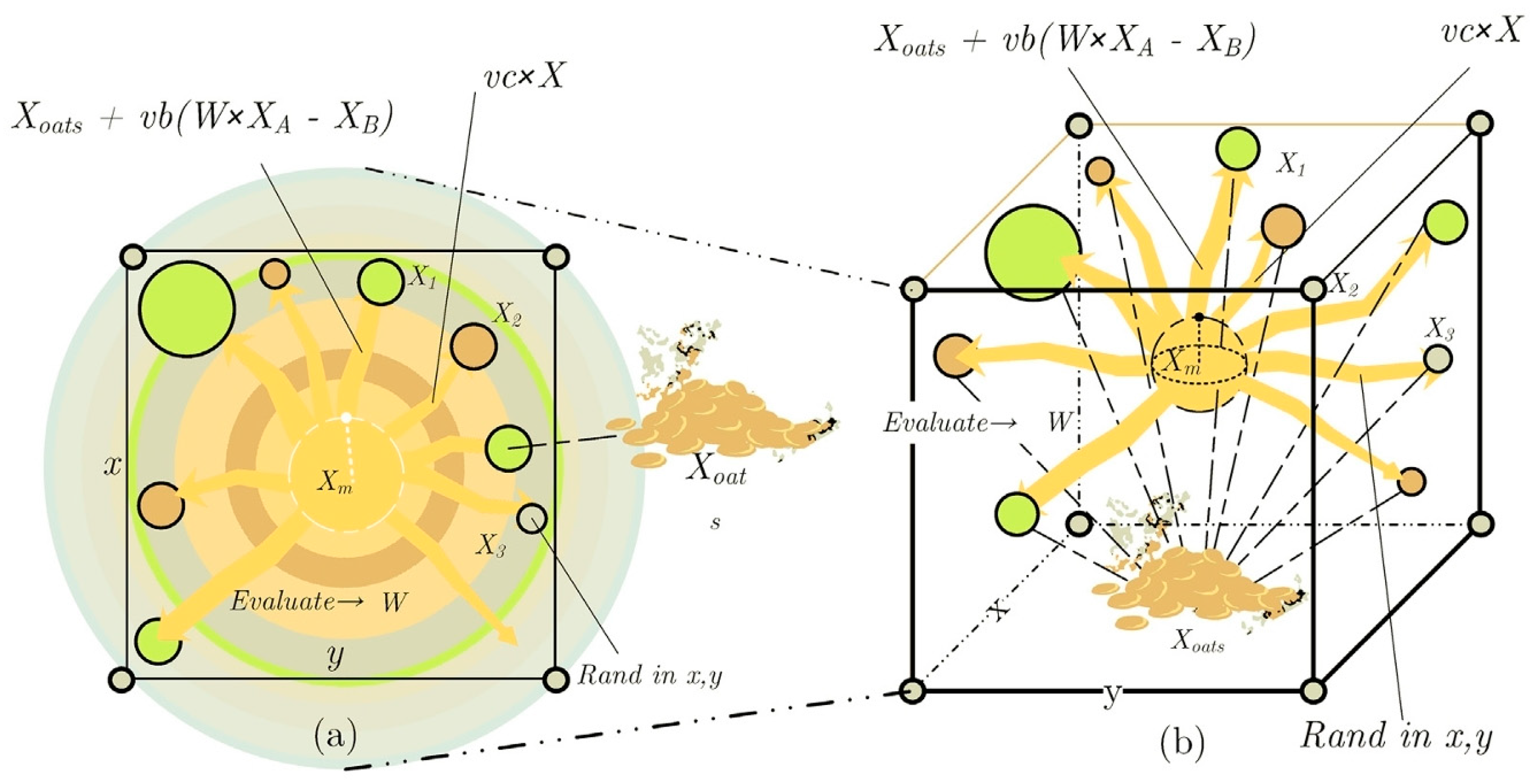
2.2. Exploration Phase

Slime molds use a random search strategy to explore new food sources. In addition, slime molds will leave a food source if they find a low density of food origin to explore other alternative food sources in the area. Equation (2) models the behavior of slime molds in exploring food sources.

$$X_i(\mathrm{t}+1)=\left(UB-LB\right)\ast rand(1,Dim)+LB$$

(2)

Here, $X_i\left(t+1\right)$ denotes the position of the i-th slime mold individual at the t + 1st iteration.

2.3. Exploitation Phase

The slime mold exhibits a propensity to approach sustenance in accordance with the olfactory cues present in its ambient environment. To articulate this behavioral tendency in mathematical terminology, the ensuing formulae are proffered to emulate the contraction mode:

$$X_i\left(t+1\right)=\left\{\begin{array}{rr}{X}_{oats}\left(t\right)+vb\left(t\right)\ast \left(W_{sort\left(i\right)}\left(t\right)\ast X_A\left(t\right)-X_B\left(t\right)\right),& \hspace{1em}\hspace{1em}r<p_i\left(t\right)\\ \hspace{1em}\hspace{1em}\hspace{1em}vc\left(t\right)\ast X_i\left(t\right) ,& \hspace{1em}\hspace{1em}r\ge p_i\left(t\right)\end{array}\right.$$

(3)

Here, r denotes a random value in [0, 1], t denotes the current number of iterations, $X_{oats}\left(t\right)$ denotes the location of the slime mold with the highest concentration of odor found so far, $X_i\left(t\right)$ denotes the position of the i-th slime mold at iteration t, $X_A\left(t\right)$ and $X_B\left(t\right)$ denote two individuals randomly selected from the slime molds, $W_{sort\left(i\right)}\left(t\right)$ denotes the weight of the sort(i)-th slime mold at iteration t, and sort denotes the sequence that has been ordered according to the fitness values (in the minimum problem, in ascending order). Figure 1 illustrates the effect of Equation (3).

The formula for p_i(t) is shown in Equation (4).

$$p_i\left(t\right)=\tanh \left|F_i\left(t\right)-F_{gb}\left(t\right)\right|$$

(4)

Here, i∈1, 2, …, n, $F_i\left(t\right)$ denotes the fitness value of the slime mold whose position is at $X_i\left(t\right)$, and $F_{gb}\left(t\right)$ denotes the fitness value of the slime mold whose global best position is found in 1 to t iterations.

vc(t) is calculated as shown in Equation (5).

$$vc\left(t\right)=unifrnd(-c,c,Dim)$$

(5)

Here, the function $unifrnd(-c,c,Dim)$ means to generate a random vector with Dim elements from a continuous uniform distribution with lower endpoint -c and upper endpoint c. For example, a run of the function $unifrnd(-1, 1, 5)$ might result in [0.6294, 0.8116, −0.7460, 0.8268, 0.2647]. c is calculated as shown in Equation (6).

$$c=1-{\displaystyle \frac{t}{\mathrm{m}\mathrm{a}\mathrm{x}\_t}}$$

(6)

Here, max_t denotes the maximum number of iterations.

The formula for vb(t) is shown in Equation (7).

$$vb\left(t\right)=unifrnd(-b,b,Dim)$$

(7)

$$b=\mathrm{arctanh}\left(c\right)$$

(8)

The values of the elements in vb(t) fluctuate randomly in the range [−b, b] and gradually converge to zero as the number of iterations increases. vc(t) fluctuates randomly in the range [−c, c] and eventually converges to zero. vb(t) and vc(t) synergistically mimic the selective behavior of the slime molds. vb(t) oscillates to simulate the process by which the slime mold decides whether or not to approach the food source or to seek other food sources.

Slime molds have been observed to form networks of interconnected veins during their migratory patterns. This ability enables them to utilize multiple food sources concurrently, establishing networks of veins that connect these sources. As the vein approaches the food source, the biological oscillator generates a propagating wave that increases the cytoplasmic flow through the vein. An increase in cytoplasmic flow leads to an increase in the diameter of the vein, and when the flow decreases, the vein contracts as its diameter decreases. This combination of positive and negative feedback enables slime molds to establish stronger routes where food concentrations are higher, thereby ensuring the receipt of maximum nutrient concentrations. Equation (9) mathematically models the positive feedback between the pulse width of the slime mold and the concentration of food being sampled, and the logarithmic part of the equation models the uncertainty in the venous contraction pattern. The logarithm is used to reduce the rate of change in the value so that the value of the contraction frequency does not vary too much. When the food concentration is high, the weight near that region increases; when the food concentration is low, the weight in that region decreases, causing a shift to explore other regions.

$$W_{sort\left(i\right)}\left(t\right)=\left\{\begin{array}{c}1+r\ast \log \left({\displaystyle \frac{F_b\left(t\right)-F_i\left(t\right)}{F_b\left(t\right)-F_w\left(t\right)}}+1\right) ,condition\\ 1-r\ast \log \left({\displaystyle \frac{F_b\left(t\right)-F_i\left(t\right)}{F_b\left(t\right)-F_w\left(t\right)}}+1\right) , others \end{array}\right.$$

(9)

Here, ‘condition’ denotes that the fitness value $F_i\left(t\right)$ of the slime mold individual is ranked in the top half of the population, r is a random value in the interval [0, 1], $F_b\left(t\right)$ denotes the optimal fitness value obtained during iteration t, and $F_w\left(t\right)$ denotes the worst fitness value obtained during iteration t.

$W_{sort\left(i\right)}\left(t\right)$ has been demonstrated to effectively simulate the oscillation frequency of slime molds at varying food concentrations. This enables slime molds to approach food more rapidly when the food concentration is higher and more slowly when the food concentration is lower at specific locations.

The position of the searching individual $X_i\left(t\right)$ can be updated according to the currently obtained best position $X_{oats}\left(t\right)$, and the parameters vb(t), vc(t), and $W_{sort\left(i\right)}\left(t\right)$ can change the position of the individual as well. The random values in the formulas allow the individuals to form search vectors at arbitrary angles, i.e., to search the solution space in any direction, thus making it possible for the algorithm to find the optimal solution. Figure 2 shows the process of evaluating the fitness values of slime molds.

Equation (10) reflects the behavior of slime molds in searching for and approaching food. The use of the parameter z simulates the behavior of slime molds that dynamically adjust their search pattern according to the quality of the food source. When the quality of the food source is high, the slime molds use the area-restricted search method, thus focusing their search on already found food sources. If the density of the initially discovered food source is low, the slime molds leave that food source to explore other alternative food sources in the region. When the quality of the various food sources varies, the slime mold can choose the food source with the highest concentration. Even when slime molds find higher-quality food, they do not abandon the current food source but split a portion of their biomass to utilize both food sources.

$$X_i(t+1)=\left\{\begin{array}{rr}\left(UB-LB\right)\ast rand(1,Dim)+LB,& rand<z\\ X_{oats}\left(t\right)+vb\left(t\right)\ast \left(W_{sort\left(i\right)}\left(t\right)\ast X_A\left(t\right)-X_B\left(t\right)\right),& r<p_i\left(t\right)\\ vc\left(t\right)\ast X_i\left(t\right),& r\ge p_i\left(t\right)\end{array}\right.$$

(10)

The parameter z is in the range [0, 0.1] and can take different values of z depending on the specific problem. Li et al. cleverly used the relationship between the magnitude of the parameter z and the random value rand to mimic the behavior of slime molds dynamically adjusting their search patterns according to the quality of the food source. A randomized strategy was used in the exploration phase to access as much of the problem space as possible. In addition, two exploitation strategies are used corresponding to the behavior of slime molds that can utilize two food sources at the same time, and the relationship between the magnitude of the parameter $p_i\left(t\right)$ and the random value r is used to decide which strategy to use. Li et al. [5] experimentally demonstrated that the algorithm results are better when z takes the value of 0.03 as this probability maintains the balance between exploration and exploitation.

2.4. Pseudo-Code of the SMA Algorithm

According to the above description, it can be seen that the algorithm first uses a randomized strategy to obtain an initialized population, then updates the location and fitness information of the slime molds according to the corresponding strategy in max_t iterations, which mimics the process of the slime molds to find good-quality food. In each iteration, the value of W is first calculated. After obtaining information about the new location and fitness value of the slime mold according to the above strategies, the information about the globally optimal slime mold individual is updated if a better slime mold individual is found in the current population. Subsequently, the next round of iterative process is started until max_t iterations are reached, then the information of the globally optimal slime mold is outputted. Algorithm 1 provides the pseudo-code of the SMA algorithm.

Algorithm 1: Pseudo-Code of SMA

Initialize the parameters popsize, Max_iteraition, Dim.

Initialize the positions of slime mold Xinitial.

While(t ≤ $\mathrm{m}\mathrm{a}\mathrm{x}\_t$)

Calculate the fitness of all slime mold.

Update $F_b\left(t\right)$, $X_{oats}\left(t\right)$.

Calculate the $W_{sort\left(i\right)}\left(t\right)$ by Equation (9), (i = 1, 2,…, n).

For each search portion

Update $p_i\left(t\right)$, vb(t), vc(t).

Update position by Equation (10).

End For

t = t + 1

End While

Return: $F_b\left(\mathrm{m}\mathrm{a}\mathrm{x}\_t\right)$, $X_{oats}\left(\mathrm{m}\mathrm{a}\mathrm{x}\_t\right)$.

3. MSSMA

This section will both describe the MSSMA improvement strategy in three points as well as describe the MSSMA process.

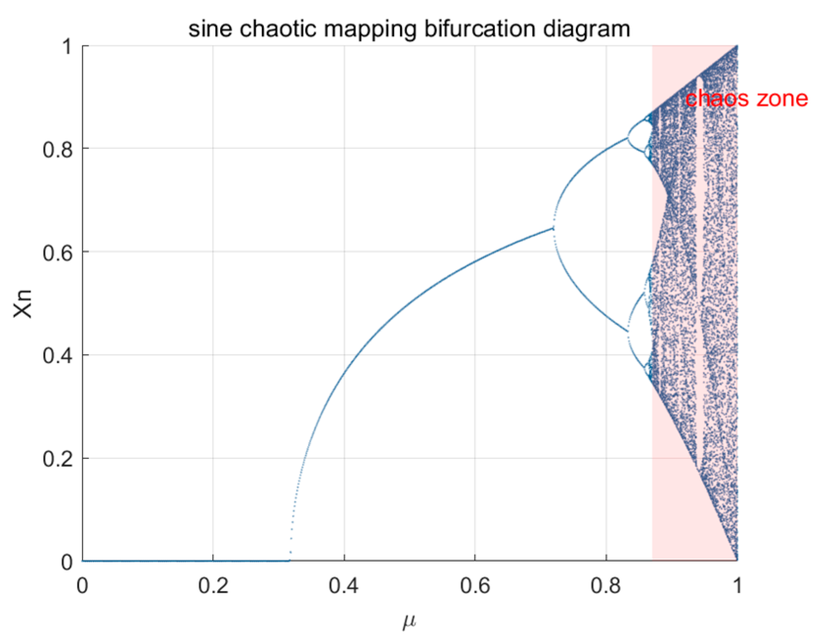
3.1. Chaotic Mapping and Reverse Learning

The randomness and uncertainty of the initial population generated by the random initialization strategy are large. The optimization and convergence performance of the algorithms is improved by improving the initial population strategy, which enhances the ability of local exploitation and global exploration [9]. In their seminal work, Maaranen and colleagues advanced the initialization population of the algorithm through the implementation of quasi-random sequences, exhibiting favorable uniform distribution characteristics. This enhancement enabled the subsequent progression of the algorithm [10]. Poles et al. demonstrated that a uniformly distributed initial population accelerates the convergence of the algorithm [11]. Ibada Ali et al. proved that in almost all cases, a better initial population will lead to faster convergence and better convergence accuracy [12]. Chaos mapping is a kind of nonlinear phenomenon that exists universally in nature because of the characteristics of randomness, ergodicity, and regularity of chaotic variables; it is often widely used in the generation of the initial population of optimization algorithms, which not only makes the initial population distribution of the algorithm more uniform but also expands the algorithm’s range of searching for the optimal outcome and improves the algorithm’s ability to escape from the local extremes. Sine chaotic mapping has the characteristics of simple structure, high efficiency, and so on [13]. The formula is shown in Equation (11). Sine chaotic mapping has better chaotic properties, and its chaoticness is strongly related to the value of the parameter $\mu$. The value of μ is [0, 1]. As shown in Figure 3, the closer μ is to 1, the better the chaotic properties are [14].

$$X_{n+1}=\mu \sin \left(\pi X_n\right),a\in \left[\mathrm{0,1}\right]$$

(11)

The main idea of the reverse learning strategy is to generate the inverse solution of the feasible solution and select a better candidate solution by evaluating the feasible solution and the inverse solution. Ewees et al. proposed a new Quasi-Reflective Learning Mechanism (QRBL) [15], where the quasi-reflective solution is obtained based on the current solution as shown in Equation (12).

$$X_{QRBL}\left(t\right)=rand\left({\displaystyle \frac{UB+LB}{2}}, X\left(t\right)\right)$$

(12)

Here, X_QEBL(t) denotes the quasi-reflective learning solution based on the current solution X(t).

In this paper, Sine chaotic mapping is combined with quasi-reflective learning to replace the random initialization strategy of the SMA algorithm. Sine chaotic mapping is used to generate a population P1 of N individuals, and quasi-reflective learning is used to generate a population P2 of N individuals on the basis of P1, and then the 2*N individuals are ranked in terms of fitness, and the first N individuals with better fitness values are selected as the initial population.

3.2. Balancing Factor B

The parameter z is used in the viscous bacteria optimization algorithm to keep the algorithm in the balance between exploration and exploitation, and the algorithm’s proponents have concluded, through experiments, that the algorithm obtains better results when z takes the value of 0.03. However, different z values need to be set for different problems, and for intelligent optimization algorithms, it is always hoped that the algorithm will carry out more global searches in the early iteration and more local searches in the late iteration so as to accelerate the convergence of the algorithm [16,17]. For this reason, a new balancing factor B is proposed in this paper, which enables the algorithm to better maintain the balance between exploration and exploitation.

In the mucilage optimization algorithm, in order to calculate the weights of the individuals, it is necessary to sort the population individuals according to the fitness value (ascending order in the minima problem) after each population position update. In order to strengthen the global optimization seeking ability of the mucilage algorithm, a balancing factor B is introduced, and the population is divided according to the value of B to perform different position update strategies. When the individual sorted order sort(i) satisfies sort(i) > B, the global search strategy perturbed with random individuals is executed; otherwise, the individual positions are still updated with $X_{oats}\left(t\right)$, and the expression of B is as follows:

$$B=⌊{\displaystyle \frac{t}{T}}\times N\times rand⌋$$

(13)

Moreover, in randomized search, the distance moved must be randomly long or short. For this reason, Lévy flight is introduced; this is a model of random walks whose step lengths obey a Lévy distribution. Unlike traditional random walks (e.g., Brownian motion), the step lengths of Lévy flights are heavy-tailed, i.e., most of the steps are short, but occasionally, very long steps occur. This property gives Lévy flight a wide range of applications in nature and in optimization algorithms. Meanwhile, Minh et al. proposed a fast algorithm with high accuracy in the K-mean optimization algorithm (KO) [18], which generates random step lengths Levy_S using a random parameter β, which is shown in Equation (14). Figure 4 illustrates the distribution of step size Levy_S in two dimensions for different β-parameters. If β is a smaller scalar number, Levy_S will reach a longer move and vice versa, and if β is a larger numerical scalar, Levy_S will reach a shorter move. The objective of expanding the search space through random steps, with varying lengths, and incorporating additional random movements, is achieved when β takes the value in Equation (14).

$$Levy\_S={\displaystyle \frac{U}{{\left|V\right|}^{\raisebox{1ex}{$1$}\!\left/ \!\raisebox{-1ex}{$\beta $}\right.}}} , \beta =1+rand$$

(14)

Here, U and V are two normal distribution variables with standard deviations of σ_u and σ_v as given in Equations (15) and (16).

$$\begin{array}{c}U=normal\left(0,{\sigma }_u^2\right)\\ {\sigma }_u={\left\{{\displaystyle \frac{f\left(1+\beta \right)\sin \left(\pi \beta /2\right)}{f\left[\left(1+\beta \right)/2\right]\beta 2^{\left(\beta -1\right)/2}}}\right\}}^{1/\beta },1\le \beta \le 2\end{array}$$

(15)

$$\begin{array}{c}V=normal\left(0,{\sigma }_v^2\right)\\ {\sigma }_v=1\end{array}$$

(16)

In Equation (15), the Gamma function f for an integer z is expressed as in Equation (17).

$$f\left(z\right)={\int }_0^{\infty }{t}^{z-1}{e}^t dt$$

(17)

Based on the above strategy, a new global search strategy is obtained as shown in Equation (18).

$$X\left(t+1\right)=X\left(t\right)+Levy\_S$$

(18)

3.3. Elite Tangent Search Strategy

Sticky fungus optimization algorithms have the advantages of strong global search capability and easy parallelization, but they also have the disadvantages of insufficient local exploitation capability and tendency to fall into local optima. A Layeb proposes the Tangent Search Algorithm (TSA) inspired by the tangent function [19], which has strong global search capability and a fast convergence speed. With reference to the tangent search strategy and improvements, a new elite tangent search strategy is proposed as illustrated in Equation (19). By introducing the tangent search strategy around the optimal individual, the local exploitation ability of the algorithm can be significantly enhanced, and the information of the optimal individual can be utilized to guide the search direction so as to approximate the global optimal solution faster [20,21]. Meanwhile, the tangent search strategy can avoid the inefficiency of random search, reduce the invalid search, and improve the convergence speed. This new strategy not only retains the global exploration advantage of the slime mold algorithm but also makes up for its lack of exploitation capability through local refinement search, thus achieving a better performance balance in complex optimization problems.

$$X\left(t+1\right)=\left\{\begin{array}{l}{X}_b\left(t\right)+step\times \tan \left(\omega \right)\times \left(X_b\left(t\right)\times rand\left(\mathrm{0,1}\right)-X\left(t\right)\right) X\left(t\right)=X_b\left(t\right)\\ X_b\left(t\right)+step\times \tan \left(\omega \right)\times \left(X_b\left(t\right)-X\left(t\right)\right) X\left(t\right)\ne X_b\left(t\right)\end{array}\right.$$

(19)

Here, the parameters ω and step are shown in Equations (20) and (21), respectively.

$$\omega ={\displaystyle \frac{rand(0, 1)\times \pi }{2.1}}$$

(20)

$$step=10\times sign(rand\left(0, 1\right))\times norm(\overrightarrow{X_b\left(t\right)})\times \log (1+{\displaystyle \frac{10\times dim}{t}})$$

(21)

Here, sign() is the sign function, norm() is the Euclidean paradigm, and dim denotes the dimension of the search space.

Specifically, by recording the optimal value of best(t) at each iteration, when the optimal value of the result of L calculations is constant, the population is divided, and the top half of the individuals with the best fitness values are classified as the elite subpopulation, and the positions of the individuals are updated using a new elite tangent search strategy, which enhances the algorithm’s ability to develop locally. The value of L has an important impact on the performance and efficiency of the algorithm. A smaller value of L causes the algorithm to execute the elite tangent search strategy more frequently, which speeds up the local exploitation capability and helps converge quickly in the early stages; however, too-frequent elite search may cause the algorithm to fall into a local optimum prematurely, reducing the global exploration capability and increasing the computational cost. On the contrary, a larger L-value delays the triggering of the elite search, allowing the algorithm more time for global exploration, which makes it more likely to find the global optimal solution, but may reduce the convergence speed. Therefore, the choice of L needs to strike a balance between global exploration and local exploitation, and the specific value should be adjusted according to the complexity of the problem and the characteristics of the search space, and it has been concluded through experiments that the algorithm achieves better results when the value of L is 3.

3.4. Pseudo-Code of the MSSMA Algorithm

Based on the use of the above three strategies, the individual location update public for the MSSMA is obtained as shown in Equation (22).

$$X(t+1)=\left\{\begin{array}{c} \left\{\begin{array}{cc}rand\ast \left(UB-LB\right)+LB ,\hfill & r1\le 0.5 \\ X(t)+Levy\left(S\right) ,\hfill & r1>0.5\end{array}\right. \mathrm{sort}(i)>B \hfill \\ \left\{\begin{array}{c}{X}_b\left(t\right)+vb\ast (W\ast X_A\left(t\right)-X_B\left(t\right)), r2<p \\ vc\ast X\left(t\right), r2\ge p \end{array} \mathrm{s}\mathrm{o}\mathrm{r}\mathrm{t}(\mathrm{i})\le B\right.\end{array} \right.$$

(22)

Here, r1 and r2 denote random values in the interval [0, 1], and i denotes the ordinal number of the individual $X\left(t\right)$ in the sorted population.

The pseudo-code of the MSSMA is shown in Algorithm 2.

Algorithm 2: MSSMA Pseudo-Code

Input: N,f,dim,T,LB,UB

Output: The global best solution and its fitness value

Initial populations are generated using chaotic mapping and reverse learning strategies, slime mold fitness values are calculated, and globally optimal solutions are recorded.

Population are sorted by fitness value to obtain sort(i), and slime mold weight information is updated by Equation (6)

While(t < T)

Calculate the value of B by Equation (13).

While(i < N)

Update position by Equation (22).

End While

Check if the location of the slime mold is within the search space and calculate the fitness value of the slime mold.

If a better solution is found in the current population, then update the global best solution and its fitness.

If (best(t) = best(t − L) && t > L)

Calculate the position of the slime molds that rank in the top half of the fitness values by Equation (19)

End If

Check if the location of the slime mold is within the search space and calculate the fitness value of the slime mold.

Update the optimal slime mold position and the optimal value.

Population are sorted by fitness value to obtain sort(i), and slime mold weight information is updated by Equation (6)

End While

Return: The global best solution and its fitness value.

4. Experimentation and Application

To test the performance of the MSSMA, 50 different benchmark functions (f1, f2, …, f50) were chosen as shown in

Table A1. Fifty benchmarks’ function information. D: Dimensions, C: Characteristics, U: Unimodal, M: Multimodal, S: Separable, and N: Non-separable.

C	Function	D	Range	fopt
US	$f_1\left(x\right)=25+{\sum }_{i=1}^n⌊x_i⌋$	5	[−5.12, 5.12]	−5
US	$f_2\left(x\right)={\sum }_{i=1}^n{\left(⌊x_i+0.5⌋\right)}^2$	30	[−100, 100]	0
US	$f_3\left(x\right)={\sum }_{i=1}^n{x}_i^2$	30	[−100, 100]	0
US	$f_4\left(x\right)={\sum }_{i=1}^n{i{x}_i}^2$	30	[−10, 10]	0
US	$f_5\left(x\right)={\sum }_{i=1}^n{i{x}_i}^4+random\left[0,\right.\left.1\right)$	30	[−1.28, 1.28]	0
UN	$f_6\left(x\right)={\left(1.5-x_1+x_1{x}_2\right)}^2+{\left(2.25-x_1+x_1{x}_2^2\right)}^2+{\left(2.625-x_1+x_1{x}_2^3\right)}^2$	5	[−4.5, 4.5]	0
UN	$f_7\left(x\right)=-\cos \left(x_1\right)\cos \left(x_2\right)e^{-{\left(x_1-\pi \right)}^2-{\left(x_2-\pi \right)}^2}$	2	[−100, 100]	−1
UN	$f_8\left(x\right)=0.26\left(x_1^2+x_2^2\right)-0.48x_1{x}_2$	2	[−10, 10]	0
UN	$\begin{array}{c}{f}_9\left(x\right)=100{\left(x_1-x_2\right)}^2+{\left(x_1-1\right)}^2+{\left(x_4-1\right)}^2+{90\left(x_3^2-x_4\right)}^2\\ +10.1\left[{\left(x_2-1\right)}^2+{\left(x_4-1\right)}^2\right]+19.8\left(x_2-1\right)\left(x_4-1\right)\end{array}$	4	[−10, 10]	0
UN	$f_{10}\left(x\right)={\sum }_{i=1}^n{\left(x_i-1\right)}^2+{\sum }_{i=2}^n{x}_i{x}_{i-1}$	6	[−D2, D2]	−50
UN	$f_{11}\left(x\right)={\sum }_{i=1}^n{\left(x_i-1\right)}^2+{\sum }_{i=2}^n{x}_i{x}_{i-1}$	10	[−D2, D2]	−210
UN	$f_{12}\left(x\right)={\sum }_{i=1}^n{x_i}^2+{\left({\sum }_{i=1}^{n}0.5i{x}_i\right)}^2+{\left({\sum }_{i=1}^{n}0.5i{x}_i\right)}^4$	10	[−5, 10]	0
UN	$f_{13}\left(x\right)={\sum }_{i=1}^{{\displaystyle \raisebox{1ex}{$n$}\!\left/ \!\raisebox{-1ex}{$k$}\right.}}{\left(x_{4i-3}+10x_{4i-2}\right)}^2+5{\left(x_{4i-1}+10x_{4i}\right)}^2+5{\left(x_{4i-2}+x_{4i-1}\right)}^4+{10\left(x_{4i-1}+x_{4i}\right)}^4$	24	[−4, 5]	0
UN	$f_{14}\left(x\right)={\sum }_{i=1}^n\left|x_i\right|+{\prod }_{i=1}^n\left|x_i\right|$	30	[−10, 10]	0
UN	$f_{15}\left(x\right)={\sum }_{i=1}^n{\left({\sum }_{j=1}^i{x}_j\right)}^2$	30	[−100, 100]	0
UN	$f_{16}\left(x\right)={\sum }_{i=1}^n{\left(100{\left(x_{i+1}-x_i\right)}^2\right)+\left(x_i-1\right)}^2$	30	[−30, 30]	0
UN	$f_{17}\left(x\right)={\left(x_1-1\right)}^2+{\sum }_{i=1}^{n}i{\left(2x_i^2-x_{i-1}\right)}^2$	30	[−10, 10]	0
MS	$f_{18}\left(x\right)={\left[{\displaystyle \frac{1}{500}}+{\sum }_{j=1}^{25}{\displaystyle \frac{1}{j+{\sum }_{j=1}^2{\left(x_i-a_{ij}\right)}^6}}\right]}^{-1}$	2	[−65.536, 65.536]	0.998
MS	$f_{19}\left(x\right)={\left(x_2-{\displaystyle \frac{5.1}{4{\pi }^2}}{x}_1^2+{\displaystyle \frac{5}{\pi }}{x}_1-6\right)}^2+10\left(1-{\displaystyle \frac{1}{8\pi }}\right)\cos x_1+10$	2	[−5, 10] × [0, 15]	0.398
MS	$f_{20}\left(x\right)=x_1^2+{2x}_2^2-0.3\cos \left(3\pi x_1\right)-0.4\cos \left(4\pi x_2\right)+0.7$	2	[−100, 100]	0
MS	$f_{21}\left(x\right)={\left(x_1+2x_2-7\right)}^2+{\left({2x}_1+x_2-5\right)}^2$	2	[−10, 10]	0
MS	$f_{22}\left(x\right)=-{\sum }_{i=1}^n\left[\left(x_i^2-10\cos \left(2\pi x_i\right)+10\right)\right]$	30	[−5.12, 5.12]	0
MS	$f_{23}\left(x\right)=-{\sum }_{i=1}^n\left(x_i\sin \sqrt{\left|x_i\right|}\right)$	30	[−500, 500]	−12,569.5
MS	$f_{24}\left(x\right)=-{\sum }_{i=1}^n\sin \left(x_i\right){\left(\sin \left({\displaystyle \raisebox{1ex}{$i{x}_i^2$}\!\left/ \!\raisebox{-1ex}{$\pi $}\right.}\right)\right)}^{20}$	2	[0, π]	−1.8013
MS	$f_{25}\left(x\right)=-{\sum }_{i=1}^n\sin \left(x_i\right){\left(\sin \left({\displaystyle \raisebox{1ex}{$i{x}_i^2$}\!\left/ \!\raisebox{-1ex}{$\pi $}\right.}\right)\right)}^{20}$	5	[0, π]	−4.6877
MS	$f_{26}\left(x\right)=-{\sum }_{i=1}^n\sin \left(x_i\right){\left(\sin \left({\displaystyle \raisebox{1ex}{$i{x}_i^2$}\!\left/ \!\raisebox{-1ex}{$\pi $}\right.}\right)\right)}^{20}$	10	[0, π]	−9.6602
MN	$f_{27}\left(x\right)=0.5+{\displaystyle \frac{{\mathrm{s}\mathrm{i}\mathrm{n}}^2\left(\sqrt{x_1^2+x_2^2}\right)-0.5}{{\left(1+0.001\left(x_1^2+x_2^2\right)\right)}^2}}$	2	[−100, 100]	0
MN	$f_{28}\left(x\right)=4x_1^2-2.1x_1^4+{\displaystyle \frac{1}{3}}{x}_1^6+x_1{x}_2-4x_2^2+x_2^4$	2	[−5, 5]	−1.03163
MN	$f_{29}\left(x\right)=x_1^2+{2x}_2^2-0.3\cos \left(3\pi x_1\right)\left(4\pi x_3\right)+0.3$	2	[−100, 100]	0
MN	$f_{30}\left(x\right)=x_1^2+{2x}_2^2-0.3\cos \left(3\pi x_1+4\pi x_3\right)+0.3$	2	[−100, 100]	0
MN	$f_{31}\left(x\right)=\left({\sum }_{i=1}^{5}i\cos \left(\left(i+1\right)x_1+i\right)\right)\left({\sum }_{i=1}^{5}i\cos \left(\left(i+1\right)x_2+i\right)\right)$	2	[−10, 10]	−186.7309
MN	$\begin{array}{l}{f}_{32}\left(x\right)=\left[1+{\left(x_1+x_2+1\right)}^2\left(19-14x_1+3x_1^2-14x_2+6x_1{x}_2+3x_2^2\right)\right]\\ \times \left[30+{\left({2x}_1-3x_2+1\right)}^2\left(18-32x_1+12x_1^2+48x_2-36x_1{x}_2+27x_2^2\right)\right]\end{array}$	2	[−2, 2]	3
MN	$f_{33}\left(x\right)={\sum }_{i=1}^{11}{\left|a_i-{\displaystyle \frac{x_i\left(b_i^2+b_i{x}_2\right)}{b_i^2+b_i{x}_3+x_4}}\right|}^2$	4	[−5, 5]	0.00031
MN	$f_{34}\left(x\right)=-{\sum }_{i=1}^5{\left|\left({x_i-a}_i\right){\left({x_i-a}_i\right)}^T+c_i\right|}^{-1}$	4	[0, 10]	−10.1532
MN	$f_{35}\left(x\right)=-{\sum }_{i=1}^7{\left|\left({x_i-a}_i\right){\left({x_i-a}_i\right)}^T+c_i\right|}^{-1}$	4	[0, 10]	−10.4028
MN	$f_{36}\left(x\right)=-{\sum }_{i=1}^{10}{\left|\left({x_i-a}_i\right){\left({x_i-a}_i\right)}^T+c_i\right|}^{-1}$	4	[0, 10]	−10.5363
MN	$f_{37}\left(x\right)={\sum }_{k=1}^n{\left({\sum }_{i=1}^n\left(i^k+\beta \right)\left({\left({\displaystyle \raisebox{1ex}{$x_i$}\!\left/ \!\raisebox{-1ex}{$i$}\right.}\right)}^k-1\right)\right)}^2$	4	[−D, D]	0
MN	$f_{38}\left(x\right)={\sum }_{k=1}^n{\left(\left({\sum }_{i=1}^n{x}_i^k\right)-b_k\right)}^2$	4	[0, D]	0
MN	$f_{39}\left(x\right)=-{\sum }_{i=1}^{4}exp\left[-{\sum }_{j=1}^3{a}_{ij}{\left(x_j-p_{ij}\right)}^2\right]$	3	[0, 1]	−3.86
MN	$f_{40}\left(x\right)=-{\sum }_{i=1}^{4}exp\left[-{\sum }_{j=1}^6{a}_{ij}{\left(x_j-p_{ij}\right)}^2\right]$	6	[0, 1]	−3.32
MN	$f_{41}\left(x\right)={\displaystyle \frac{1}{4000}}{\sum }_{i=1}^n{\left(x_i-100\right)}^2-{\prod }_{i=1}^n\cos \left({\displaystyle \frac{x_i-100}{\sqrt{i}}}\right)+1$	30	[−600, 600]	0
MN	$f_{42}\left(x\right)=-20exp\left(-0.2\sqrt{{\displaystyle \frac{1}{n}}{\sum }_{i=1}^n{x}_i^2}\right)+20-e-exp\left(-{\displaystyle \frac{1}{n}}{\sum }_{i=1}^n\cos 2\pi x_i\right)$	30	[−32, 32]	0
MN	$f_{43}\left(x\right)={\displaystyle \frac{\pi }{n}}\left\{10{\mathrm{s}\mathrm{i}\mathrm{n}}^2\left(\pi y_1\right)+{\sum }_{i=1}^n{\left(y_i-1\right)}^2\left[1+10{\mathrm{s}\mathrm{i}\mathrm{n}}^2\left(\pi y_i+1\right)\right]+{\left(y_n-1\right)}^2\right\}+{\sum }_{i=1}^{30}u\left(x_i,\mathrm{10,100,4}\right)$	30	[−50, 50]	0
MN	$f_{44}\left(x\right)=0.1{\mathrm{s}\mathrm{i}\mathrm{n}}^2\left(3\pi x_1\right)+0.1{\sum }_{i=1}^{29}{\left(x_i-1\right)}^{2}p\left[1+{\mathrm{s}\mathrm{i}\mathrm{n}}^2\left(3\pi x_{i+1}\right)\right]+0.1{\left(x_n-1\right)}^2\left[1+{\mathrm{s}\mathrm{i}\mathrm{n}}^2\left(2\pi x_{30}\right)\right]+{\sum }_{i=1}^{30}u\left(x_i,\mathrm{5,100,4}\right)$	30	[−50, 50]	0
MN	$f_{45}\left(x\right)=-c_i\left(exp\left(-{\displaystyle \frac{1}{\pi }}{\sum }_{j=1}^n{\left(x_j-a_{ij}\right)}^2\right)\times \cos \left(\pi {\sum }_{j=1}^n{\left(x_j-a_{ij}\right)}^2\right)\right)$	2	[0, 10]	−1.08
MN	$f_{46}\left(x\right)=-c_i\left(exp\left(-{\displaystyle \frac{1}{\pi }}{\sum }_{j=1}^n{\left(x_j-a_{ij}\right)}^2\right)\times \cos \left(\pi {\sum }_{j=1}^n{\left(x_j-a_{ij}\right)}^2\right)\right)$	5	[0, 10]	−1.5
MN	$f_{47}\left(x\right)=-c_i\left(exp\left(-{\displaystyle \frac{1}{\pi }}{\sum }_{j=1}^n{\left(x_j-a_{ij}\right)}^2\right)\times \cos \left(\pi {\sum }_{j=1}^n{\left(x_j-a_{ij}\right)}^2\right)\right)$	10	[0, 10]	–1.080938
MN	$\begin{array}{l}\begin{array}{l}{f}_{48}\left(x\right)={\sum }_{i=1}^n{\left(A_i-B_i\right)}^2\\ A_i={\sum }_{j=1}^n\left(a_{ij}\sin {\alpha }_j+b_{ij}\cos {\alpha }_j\right)\end{array}\\ B_i={\sum }_{j=1}^n\left(a_{ij}\sin x_j+b_{ij}\cos x_j\right)\end{array}$	2	[−π, π]	0
MN	$\begin{array}{l}\begin{array}{l}{f}_{49}\left(x\right)={\sum }_{i=1}^n{\left(A_i-B_i\right)}^2\\ A_i={\sum }_{j=1}^n\left(a_{ij}\sin {\alpha }_j+b_{ij}\cos {\alpha }_j\right)\end{array}\\ B_i={\sum }_{j=1}^n\left(a_{ij}\sin x_j+b_{ij}\cos x_j\right)\end{array}$	5	[−π, π]	0
MN	$\begin{array}{l}\begin{array}{l}{f}_{50}\left(x\right)={\sum }_{i=1}^n{\left(A_i-B_i\right)}^2\\ A_i={\sum }_{j=1}^n\left(a_{ij}\sin {\alpha }_j+b_{ij}\cos {\alpha }_j\right)\end{array}\\ B_i={\sum }_{j=1}^n\left(a_{ij}\sin x_j+b_{ij}\cos x_j\right)\end{array}$	10	[−π, π]	0

in Appendix A and can be found in [22], where their detailed information can be found. This test set covers functions with four characteristics: single-peaked functions, multi-peaked functions, non-separable functions, and separable functions. Single-peaked functions have only one localized extreme while multi-peaked functions have multiple localized extremes. The multi-peak characteristic tends to make it easy for the algorithm to obtain a locally optimal solution. Separability shows that the variables of a function can be decomposed into a product of the functions of each variable, whereas indivisibility does not, because of the interconnections between their variables. This indivisibility property often leads to global optimal solutions that are difficult to find. Appendix A lists these functions, of which 17 are single-peaked, 33 are multi-peaked, 36 are indivisible, and 14 are separable.

In order to ensure the fairness of the test, the following experiments were tested using Matlab R2020a; the number of populations of the algorithms was 50, the maximum number of iterations was 1000, each algorithm was tested independently for 30 times, and the mean and variance of each method in different benchmark test functions were calculated. The test environment was a Windows 10 64 bit system with 16 GB of RAM and an Intel(R) Core(TM) i5-8250U CPU @ 1.60 GHz 1.80 GHz.

Before our experiments, we referred to many research results, and most of the comparison experiments used the classical paradigm of the same population size and number of iterations. This was because CPU time measurements are significantly affected by non-algorithmic factors such as the hardware configuration and programming language implementation differences. Whereas the number of fitness evaluations is strongly correlated with the convergence characteristics of the algorithms, enforcing a uniform number of evaluations would result in certain algorithms with adaptive iteration mechanisms not being able to take advantage of their design, creating a new unfairness. However, simply using the same population size and number of iterations does not ensure a completely fair comparison, especially when the amount of computation required for each iteration may be quite different for different algorithms, which was a major shortcoming of our experiments. Researchers should use different experimental designs depending on different application scenarios. We considered parallel computing for intelligent optimization algorithms, where the computational resources required by the algorithms do not differ much in parallel computing scenarios. Therefore, we still considered keeping the existing experimental design.

4.1. Sensitivity Analysis of Parameter L

In order to calculate the effect of parameter L on the experimental results, five representative values of L were tested, namely, L = 3, 5, 10, 15, and 20.

Table A2. Experimental results of MSSMA using different values of L (each winner is shown in bold).

ID	Index	L = 3	L = 5	L = 10	L = 15	L = 20
F1	Mean	−5.00	−5.00	−5.00	−5.00	−5.00
	Std	0.00	0.00	0.00	0.00	0.00
F2	Mean	0.00	0.00	0.00	0.00	0.00
	Std	0.00	0.00	0.00	0.00	0.00
F3	Mean	0.00	0.00	4.50 × 10−255	4.40 × 10−174	4.00 × 10−161
	Std	0.00	0.00	0.00	0.00	0.00
F4	Mean	0.00	0.00	1.90 × 10−226	1.70 × 10−191	3.40 × 10−151
	Std	0.00	0.00	0.00	0.00	3.40 × 10−300
F5	Mean	5.47 × 10−49	2.23 × 10−3	2.34 × 10−3	3.28 × 10−3	2.83 × 10−3
	Std	3.30 × 10−18	3.66 × 10−6	3.77 × 10−6	1.25 × 10−5	7.13 × 10−6
F6	Mean	6.75 × 10−10	1.21 × 10−10	2.06 × 10−10	1.85 × 10−10	3.96 × 10−10
	Std	1.15 × 10−18	1.16 × 10−19	1.94 × 10−19	1.42 × 10−19	3.41 × 10−19
F7	Mean	−1.00	−9.99 × 10−1	−9.97 × 10−1	−9.98 × 10−1	−9.97 × 10−1
	Std	1.51 × 10−20	6.18 × 10−7	1.50 × 10−4	1.81 × 10−5	1.65 × 10−4
F8	Mean	0.00	0.00	0.00	5.20 × 10−262	2.40 × 10−214
	Std	0.00	0.00	0.00	0.00	0.00
F9	Mean	4.81 × 10−7	8.63 × 10−5	5.16 × 10−5	7.49 × 10−5	4.84 × 10−5
	Std	1.50 × 10−12	2.63 × 10−8	1.85 × 10−8	3.58 × 10−8	1.37 × 10−8
F10	Mean	−5.00 × 101	−4.99 × 101	−4.99 × 101	−4.99 × 101	−4.99 × 101
	Std	1.11 × 10−18	1.99 × 10−8	8.07 × 10−8	9.7 × 10−8	5.53 × 10−7
F11	Mean	−2.10 × 102	−2.10 × 102	−2.10 × 102	−2.10 × 102	−2.10 × 102
	Std	1.92 × 10−9	1.40 × 10−2	1.26 × 10−2	3.71 × 10−2	1.01 × 10−1
F12	Mean	0.00	0.00	4.90 × 10−160	9.70 × 10−115	7.91 × 10−86
	Std	0.00	0.00	0.00	2.80 × 10−227	1.90 × 10−169
F13	Mean	0.00	0.00	1.70 × 10−223	4.80 × 10−115	2.10 × 10−116
	Std	0.00	0.00	0.00	7.00 × 10−228	1.30 × 10−230
F14	Mean	0.00	9.98 × 10−94	2.99 × 10−67	2.09 × 10−36	1.59 × 10−35
	Std	0.00	2.95 × 10−185	1.40 × 10−132	1.31 × 10−70	6.44 × 10−69
F15	Mean	0.00	2.79 × 101	6.41 × 101	6.47 × 101	4.94 × 101
	Std	0.00	2.28 × 104	5.65 × 104	7.44 × 104	1.925 × 104
F16	Mean	2.28 × 10−8	1.51	2.22	1.27	1.90
	Std	3.26 × 10−9	8.53	1.30 × 104	2.39	9.66
F17	Mean	3.46 × 10−4	5.64 × 10−1	5.80 × 10−1	6.00 × 10−1	5.80 × 10−1
	Std	4.17 × 10−13	8.34 × 10−2	9.38 × 10−2	9.07 × 10−2	1.06 × 10−1
F18	Mean	9.98 × 10−1	9.98 × 10−1	9.98 × 10−1	9.98 × 10−1	9.98 × 10−1
	Std	1.86 × 10−26	4.14 × 10−25	2.66 × 10−25	1.21 × 10−24	8.70 × 10−24
F19	Mean	3.98 × 10−1	3.98 × 10−1	3.98 × 10−1	3.98 × 10−1	3.98 × 10−1
	Std	1.10 × 10−18	3.16 × 10−20	1.05 × 10−20	3.21 × 10−17	4.70 × 10−17
F20	Mean	0.00	0.00	0.00	0.00	0.00
	Std	0.00	0.00	0.00	0.00	0.00
F21	Mean	9.58 × 10−11	9.50 × 10−12	2.26 × 10−11	1.31 × 10−11	1.89 × 10−11
	Std	1.61 × 10−20	2.68- × 10−22	4.19 × 10−21	4.58 × 10−22	7.66 × 10−22
F22	Mean	0.00	0.00	0.00	0.00	0.00
	Std	0.00	0.00	0.00	0.00	0.00
F23	Mean	−1.59 × 105	−1.88 × 105	−2.01 × 105	−2.29 × 105	−2.03 × 105
	Std	1.28 × 10−2	2.01	1.61	0.42	4.61
F24	Mean	−1.80	−1.80	−1.80	−1.80	−1.80
	Std	2.86 × 10−23	3.52 × 10−23	3.76 × 10−21	2.15 × 10−21	5.09 × 10−22
F25	Mean	−4.58	−4.46	−4.42	−4.58	−4.54
	Std	1.27 × 10−3	9.10 × 10−2	1.06 × 10−1	2.66 × 10−2	3.72 × 10−2
F26	Mean	−8.57	−7.28	−7.45	−7.61	−7.68
	Std	3.42 × 10−2	6.19 × 10−1	6.40 × 10−1	6.39 × 10−1	4.69 × 10−1
F27	Mean	0.00	0.00	0.00	0.00	0.00
	Std	0.00	0.00	0.00	0.00	0.00
F28	Mean	−1.03	−1.03	−1.03	−1.03	−1.03
	Std	1.27 × 10−25	1.17 × 10−27	4.02 × 10−27	8.42 × 10−26	1.17 × 10−24
F29	Mean	0.00	0.00	0.00	0.00	0.00
	Std	0.00	0.00	0.00	0.00	0.00
F30	Mean	0.00	0.00	0.00	0.00	0.00
	Std	0.00	0.00	0.00	0.00	0.00
F31	Mean	−1.87 × 102	−1.87 × 102	−1.87 × 102	−1.87 × 102	−1.87 × 102
	Std	4.01 × 10−14	6.43 × 10−16	8.26 × 10−14	2.38 × 10−14	1.19 × 10−14
F32	Mean	3.00	3.00	3.00	3.00	3.00
	Std	1.23 × 10−26	1.75 × 10−24	1.07 × 10−23	1.8 × 10−22	3.07 × 10−22
F33	Mean	3.08 × 10−4	3.51 × 10−4	3.37 × 10−4	4.60 × 10−4	4.49 × 10−4
	Std	5.99 × 10−14	2.83 × 10−8	5.00 × 10−9	5.99 × 10−8	6.12 × 10−8
F34	Mean	−1.02 × 101	−1.02 × 101	−1.02 × 101	−1.02 × 101	−1.02 × 101
	Std	1.26 × 10−13	6.64 × 10−13	9.13 × 10−13	4.15 × 10−12	7.79 × 10−13
F35	Mean	−1.04 × 101	−1.04 × 101	−1.04 × 101	−1.04 × 101	−1.04 × 101
	Std	4.05 × 10−12	3.84 × 10−13	2.28 × 10−12	8.58 × 10−12	1.36 × 10−11
F36	Mean	−1.05 × 101	−1.04 × 101	−1.04 × 101	−1.04 × 101	−1.04 × 101
	Std	4.70 × 10−12	4.30 × 10−13	7.13 × 10−13	1.8 × 10−12	1.38 × 10−11
F37	Mean	9.26 × 10−2	6.75 × 10−2	2.18 × 10−2	5.75 × 10−2	5.59 × 10−2
	Std	1.91 × 10−2	2.06 × 10−2	1.97 × 10−3	2.08 × 10−2	2.05 × 10−2
F38	Mean	9.57 × 10−4	3.30 × 10−4	5.58 × 10−4	7.98 × 10−4	7.19 × 10−4
	Std	1.53 × 10−6	2.15 × 10−7	1.46 × 10−6	1.54 × 10−6	1.48 × 10−6
F39	Mean	−3.86	−3.86	−3.86	−3.86	−3.86
	Std	9.69 × 10−22	3.30 × 10−22	2.06 × 10−21	1.02 × 10−18	3.23 × 10−18
F40	Mean	−3.28	−3.20	−3.21	−3.20	−3.21
	Std	2.34 × 10−5	1.74 × 10−14	9.10 × 10−4	8.08 × 10−11	9.10 × 10−4
F41	Mean	0.00	1.10 × 10−4	0.00	0.00	2.33 × 10−10
	Std	0.00	3.65 × 10−7	0.00	0.00	1.64 × 10−18
F42	Mean	3.89 × 10−16	4.44 × 10−16	4.47 × 10−16	4.59 × 10−16	4.87 × 10−16
	Std	0.00	0.00	0.00	0.00	0.00
F43	Mean	2.36 × 10−8	3.45 × 10−5	2.20 × 10−5	4.07 × 10−5	2.73 × 10−5
	Std	4.30 × 10−11	7.54 × 10−9	1.88 × 10−9	9.11 × 10−9	1.57 × 10−9
F44	Mean	1.07 × 10−3	6.93 × 10−3	8.26 × 10−3	8.50 × 10−3	7.13 × 10−3
	Std	5.03 × 10−6	1.92 × 10−4	3.82 × 10−4	3.23 × 10−4	2.49 × 10−4
F45	Mean	−1.08	−1.08	−1.08	−1.08	−1.08
	Std	2.33 × 10−20	1.44 × 10−20	1.21 × 10−20	9.76 × 10−20	2.90 × 10−20
F46	Mean	−1.40	−1.09	−1.18	−1.26	−1.17
	Std	5.40 × 10−3	1.78 × 10−1	8.41 × 10−2	8.20 × 10−2	1.06 × 10−1
F47	Mean	−9.40 × 10−1	−3.17 × 10−1	−2.88 × 10−1	−2.78 × 10−1	−2.07 × 10−1
	Std	5.57 × 10−5	3.58 × 10−2	2.94 × 10−2	2.20 × 10−2	2.82 × 10−2
F48	Mean	2.85 × 10−9	1.78 × 10−9	3.39 × 10−9	5.97 × 10−9	8.15 × 10−9
	Std	3.33 × 10−17	4.1810−18	1.29 × 10−17	6.24 × 10−17	1.99 × 10−16
F49	Mean	1.04 × 102	2.49 × 102	1.34 × 102	1.72 × 102	3.17 × 102
	Std	2.45 × 105	3.56 × 105	8.26 × 105	8.88 × 105	4.06 × 105
F50	Mean	3.83 × 103	4.42 × 105	4.12 × 105	2.05 × 105	3.00 × 105
	Std	4.86 × 106	4.38 × 107	1.20 × 107	7.48 × 106	2.23 × 107

in Appendix A provides the experimental data for the different values of L, where the best results have been highlighted in bold.

The results of the Friedman test for the algorithm using different values of L are displayed in

Table 1. Results of Friedman test for MSSMA at different values of L.

ID	L = 3	L = 5	L = 10	L = 15	L = 20
(W|T|L)	(40|6|4)	(20|26|4)	(11|35|4)	(8|32|10)	(7|24|19)
Ave	1.56	2.88	3.54	3.40	3.62
Rank	1	2	3	4	5

. (W|T|L) denote the number of algorithms achieving the best, average, and worst performance in the test set, respectively. Ave represents the average Friedman mean ranking and Rank shows the ranking values of all competitors. Lower values of Ave correspond to superior overall performance metrics of the algorithm in question. The results indicate that when L is taken to be 3, the MSSMA has forty wins, four ties, and four losses, with a Friedman mean ranking value of 1.56, ranking first. Therefore, the value of L in this paper is 3.

4.2. Ablation Experiment

An ablation experiment is a research method that evaluates the contribution of a specific component in a model by systematically removing or modifying it. The basic principle is to reveal the role of the target component by comparing the performance difference between the baseline model and the ablation model. During the experiment, a complete baseline model is first constructed, followed by removing or adjusting the module, parameter, or strategy to be studied while keeping all other conditions constant and observing the change in model performance. If there is a significant decrease in performance after ablation, it indicates that the component is critical to the system; if the effect is weak, it may imply that it is redundant or needs to be optimized. Ablation experiments are necessary because they help researchers to test hypotheses, rule out invalid designs, and improve the interpretability of models. The swarm intelligence optimization algorithm can be divided into three parts, initialization, exploitation, and exploration, and we propose an improvement for each of these three parts (chaotic initialization, a balancing factor, and an elite tangent strategy). In order to verify the effectiveness of the improvement measures, the following three comparison algorithms were designed by deleting one of the improvement measures based on the MSSMA:

MSSMA-1: delete elite tangent strategy;

MSSMA-2: delete balancing factor;

MSSMA-3: remove chaotic initialization.

Table A3. Experimental data of ablation experiments (each winner is shown in bold).

ID	Index	MSSMA	SMA	MSSMA-1	MSSMA-2	MSSMA-3
F1	Mean	−5.00	−5.00	−5.00	−5.00	−5.00
	Std	0.00	0.00	0.00	0.00	0.00
F2	Mean	0.00	0.00	0.00	0.00	0.00
	Std	0.00	0.00	0.00	0.00	0.00
F3	Mean	0.00	0.00	1.49 × 10−4	0.00	0.00
	Std	0.00	0.00	2.04 × 10−7	0.00	0.00
F4	Mean	0.00	0.00	1.13 × 10−2	0.00	0.00
	Std	0.00	0.00	8.73 × 10−4	0.00	0.00
F5	Mean	5.47 × 10−8	3.26 × 10−4	1.92 × 10−4	1.81 × 10−6	4.27 × 10−7
	Std	3.30 × 10−18	5.45 × 10−8	2.11 × 10−6	1.84 × 10−8	8.01 × 10−8
F6	Mean	6.75 × 10−10	2.85 × 10−8	1.15 × 10−8	3.99 × 10−9	7.76 × 10−10
	Std	1.15 × 10−18	2.80 × 10−14	9.29 × 10−14	9.26 × 10−23	3.25 × 10−18
F7	Mean	−1.00	−9.95 × 10−1	−9.97 × 10−1	−1.00	−1.00
	Std	1.51 × 10−20	5.76 × 10−4	2.06 × 10−10	6.15 × 10−24	4.92 × 10−19
F8	Mean	0.00	0.00	9.89 × 10−189	0.00	0.00
	Std	0.00	0.00	0.00	0.00	0.00
F9	Mean	4.81 × 10−7	2.37 × 10−4	4.01 × 10−5	1.72 × 10−4	7.37 × 10−7
	Std	1.50 × 10−12	2.34 × 10−7	1.52 × 10−9	7.91 × 10−8	2.53 × 10−12
F10	Mean	−5.00 × 101	−5.00 × 101	−5.00 × 101	−5.00 × 101	−5.00 × 101
	Std	1.11 × 10−18	8.08 × 10−9	3.63 × 10−9	8.15 × 10−10	4.53 × 10−15
F11	Mean	−2.10 × 102	−2.10 × 102	−2.10 × 102	−2.10 × 102	−2.10 × 102
	Std	1.92 × 10−9	2.39 × 10−4	6.81 × 10−4	1.15 × 10−8	3.25 × 10−9
F12	Mean	0.00	0.00	0.00	0.00	0.00
	Std	0.00	0.00	0.00	0.00	0.00
F13	Mean	0.00	0.00	2.17 × 10−243	0.00	0.00
	Std	0.00	0.00	0.00	0.00	0.00
F14	Mean	0.00	3.42 × 10−2	1.32 × 10−2	1.07 × 10−1	0.00
	Std	0.00	1.06 × 10−2	1.78 × 10−1	2.82 × 10−1	0.00
F15	Mean	0.00	0.00	3.35 × 10−1	0.00	0.00
	Std	0.00	0.00	7.56 × 10−1	0.00	0.00
F16	Mean	2.28 × 10−6	6.85 × 101	21.04	1.03	2.33 × 10−4
	Std	3.26 × 10−9	1.20 × 104	5.52 × 10−2	4.18 × 10−1	1.32 × 10−1
F17	Mean	3.46 × 10−4	8.12 × 10−1	3.51 × 10−1	5.95 × 10−1	3.07 × 10−3
	Std	4.17 × 10−13	8.05 × 10−2	3.27 × 10−2	2.48 × 10−2	1.78 × 10−2
F18	Mean	9.98 × 10−1	9.98 × 10−1	9.98 × 10−1	9.98 × 10−1	9.98 × 10−1
	Std	1.86 × 10−26	3.00 × 10−23	3.04 × 10−24	3.27 × 10−26	1.96 × 10−26
F19	Mean	3.98 × 10−1	3.98 × 10−1	3.98 × 10−1	3.98 × 10−1	3.98 × 10−1
	Std	1.10 × 10−18	1.12 × 10−16	3.17 × 10−15	2.89 × 10−18	2.35 × 10−18
F20	Mean	0.00	0.00	0.00	0.00	0.00
	Std	0.00	0.00	0.00	0.00	0.00
F21	Mean	9.58 × 10−11	3.30 × 10−10	3.46 × 10−10	4.62 × 10−10	1.04 × 10−10
	Std	1.61 × 10−20	5.55 × 10−19	9.36 × 10−15	5.71 × 10−25	8.71 × 10−20
F22	Mean	0.00	0.00	5.04 × 10−4	0.00	0.00
	Std	0.00	0.00	1.87 × 10−16	0.00	0.00
F23	Mean	−1.59 × 105	−2.09 × 105	−2.09 × 105	−2.05 × 105	−1.84 × 105
	Std	1.28 × 10−2	1.18 × 102	1.22 × 10−2	3.69 × 10−2	1.98 × 10−2
F24	Mean	−1.80	−1.80	−1.80	−1.80	−1.80
	Std	2.86 × 10−23	1.67 × 10−17	5.81 × 10−19	5.15 × 10−20	7.81 × 10−23
F25	Mean	−4.58	−4.39	−4.45	−4.45	−4.57
	Std	1.27 × 10−3	8.90 × 10−2	3.24 × 10−2	1.15 × 10−2	1.29 × 10−2
F26	Mean	−8.57	−8.46	−8.46	−8.49	−8.54
	Std	3.42 × 10−2	5.28 × 10−1	5.03 × 10−1	5.39 × 10−1	3.32 × 10−1
F27	Mean	0.00	0.00	0.00	0.00	0.00
	Std	0.00	0.00	0.00	0.00	0.00
F28	Mean	−1.03	−1.03	−1.03	−1.03	−1.03
	Std	1.27 × 10−25	9.65 × 10−22	1.23 × 10−22	3.48 × 10−24	5.12 × 10−25
F29	Mean	0.00	0.00	0.00	0.00	0.00
	Std	0.00	0.00	0.00	0.00	0.00
F30	Mean	0.00	0.00	0.00	0.00	0.00
	Std	0.00	0.00	0.00	0.00	0.00
F31	Mean	−1.87 × 102	−1.87 × 102	−1.87 × 102	−1.87 × 102	−1.87 × 102
	Std	4.01 × 10−14	1.30 × 10−13	4.03 × 10−13	1.63 × 10−13	1.22 × 10−14
F32	Mean	3.00	3.00	3.00	3.00	3.00
	Std	1.23 × 10−26	2.97 × 10−22	1.48 × 10−22	1.06 × 10−24	4.34 × 10−25
F33	Mean	3.08 × 10−4	4.44 × 10−4	3.86 × 10−4	3.10 × 10−4	3.09 × 10−4
	Std	5.99 × 10−14	2.96 × 10−8	7.17 × 10−9	4.57 × 10−14	3.94 × 10−12
F34	Mean	−1.02 × 101	−1.02 × 101	−1.02 × 101	−1.02 × 101	−1.02 × 101
	Std	1.26 × 10−13	2.04 × 10−9	1.35 × 10−9	8.18 × 10−10	2.28 × 10−12
F35	Mean	−1.04 × 101	−1.04 × 101	−1.04 × 101	−1.04 × 101	−1.04 × 101
	Std	4.05 × 10−12	6.36 × 10−9	2.70 × 10−9	4.00 × 10−11	6.44 × 10−12
F36	Mean	−1.05 × 101	−1.05 × 101	−1.05 × 101	−1.05 × 101	−1.05 × 101
	Std	4.70 × 10−12	1.82 × 10−9	3.91 × 10−9	2.40 × 10−10	2.67 × 10−12
F37	Mean	9.26 × 10−2	1.38 × 10−1	1.02 × 10−1	9.58 × 10−2	9.43 × 10−2
	Std	1.91 × 10−2	3.77 × 10−2	1.99 × 10−2	2.57 × 10−2	2.50 × 10−2
F38	Mean	9.57 × 10−4	7.85 × 10−3	6.75 × 10−3	2.56 × 10−3	1.61 × 10−3
	Std	1.53 × 10−6	7.91 × 10−5	9.31 × 10−5	9.16 × 10−8	7.87 × 10−6
F39	Mean	−3.86	−3.86	−3.86	−3.86	−3.86
	Std	9.69 × 10−22	1.27 × 10−16	4.66 × 10−18	9.87 × 10−20	5.50 × 10−21
F40	Mean	−3.28	−3.24	−3.21	−3.24	−3.26
	Std	2.34 × 10−5	3.07 × 10−3	9.10 × 10−4	1.39 × 10−3	3.59 × 10−3
F41	Mean	0.00	0.00	7.73 × 10−7	0.00	0.00
	Std	0.00	0.00	1.20 × 10−11	0.00	0.00
F42	Mean	3.89 × 10−16	4.44 × 10−16	4.44 × 10−16	4.44 × 10−16	4.44 × 10−16
	Std	0.00	2.07 × 10−32	6.50 × 10−9	0.00	0.00
F43	Mean	2.36 × 10−8	4.08 × 10−4	4.02 × 10−6	2.22 × 10−6	1.31 × 10−7
	Std	4.30 × 10−11	1.05 × 10−6	1.20 × 10−12	9.67 × 10−8	6.30 × 10−11
F44	Mean	1.07 × 10−3	3.60 × 10−2	7.51 × 10−3	5.76 × 10−3	4.14 × 10−3
	Std	5.03 × 10−6	2.28 × 10−3	3.05 × 10−7	7.46 × 10−7	1.61 × 10−6
F45	Mean	−1.08	−1.08	−1.08	−1.08	−1.08
	Std	2.33 × 10−20	4.35 × 10−17	1.15 × 10−18	3.86 × 10−19	4.51 × 10−20
F46	Mean	−1.40	−1.55 × 10−1	−0.98	−1.03	−1.32
	Std	5.40 × 10−3	9.16 × 10−2	1.41 × 10−2	1.04 × 10−2	7.12 × 10−2
F47	Mean	−9.40 × 10−1	−1.37 × 10−3	−1.35	−1.34	−1.24
	Std	5.57 × 10−5	3.32 × 10−4	1.94 × 10−4	6.4 × 10−3	4.52 × 10−4
F48	Mean	2.85 × 10−9	1.46 × 10−8	7.44 × 10−9	7.23 × 10−9	3.44 × 10−9
	Std	3.33 × 10−17	3.24 × 10−16	9.31 × 10−11	9.72 × 10−21	3.08 × 10−17
F49	Mean	1.04 × 102	2.82 × 102	1.31 × 102	1.22 × 102	1.19 × 102
	Std	2.45 × 105	5.67 × 105	1.87 × 105	5.18 × 105	6.53 × 105
F50	Mean	3.83 × 103	5.17 × 103	4.59 × 103	4.09 × 103	3.86 × 103
	Std	4.86 × 106	6.29 × 106	2.58 × 106	5.41 × 106	7.82 × 106

shows the experimental data for the five algorithms on a test set consisting of 50 benchmark functions, with the best results highlighted in bold. From the results of the experiments shown in

Table 2. Results of Friedman test for ablation experiments.

ID	MSSMA	SMA	MSSMA-1	MSSMA-2	MSSMA-3
(W|T|L)	(49|1|0)	(14|9|27)	(7|31|12)	(15|35|0)	(17|33|0)
Ave	1.68	3.20	3.54	3.40	3.14
Rank	1	3	5	4	2

, it can be seen that the performance of the algorithms decreases after the removal of a certain improvement measure, and the performance of the algorithms can only be improved by using all three improvement measures simultaneously.

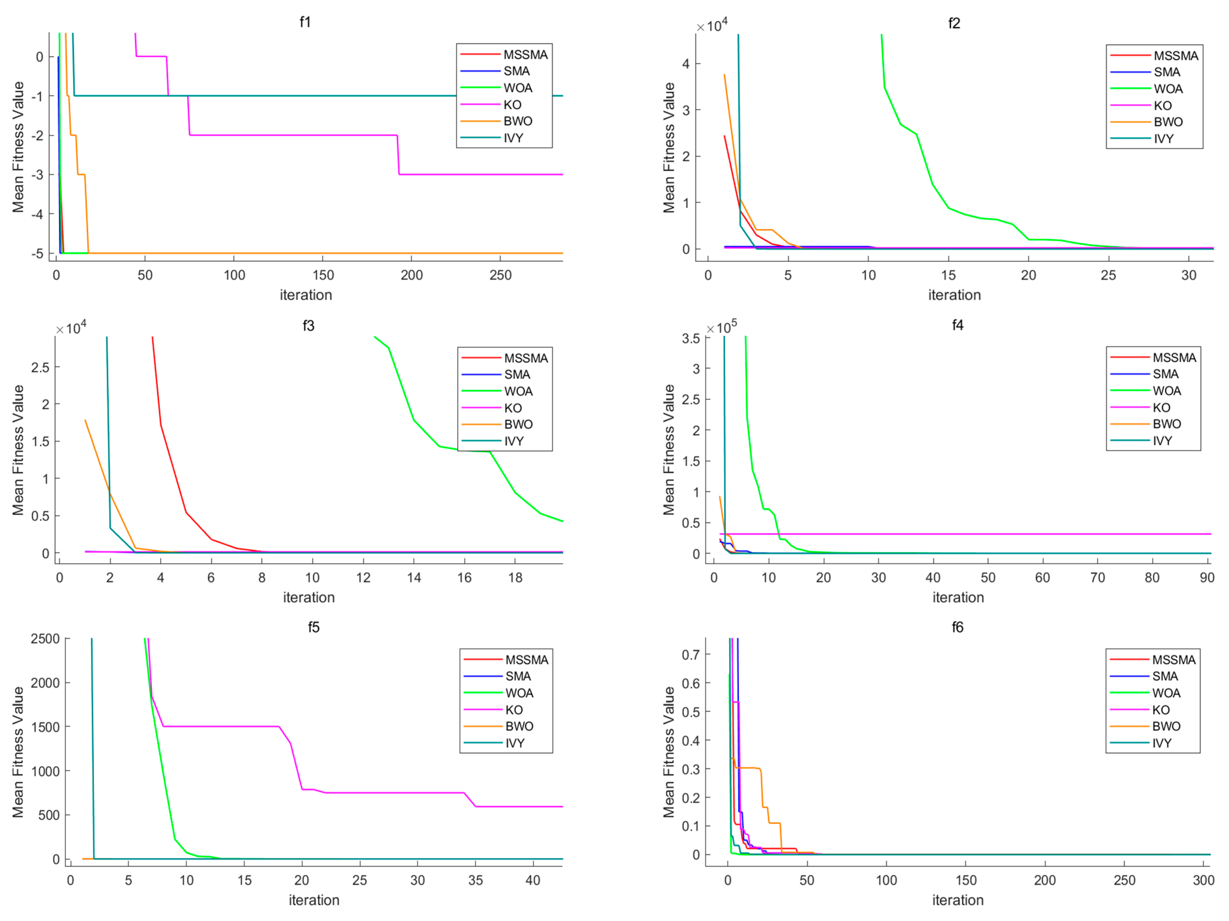
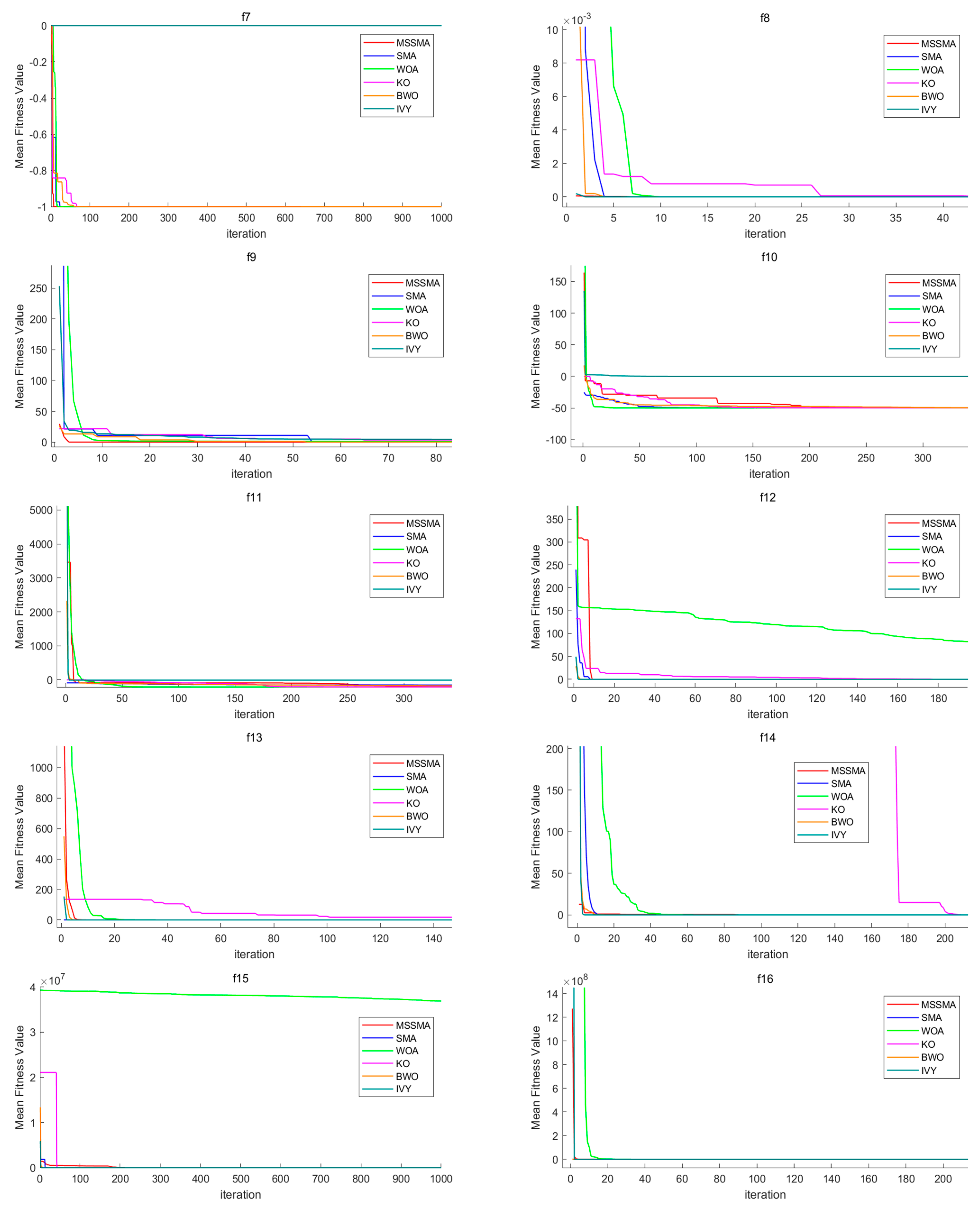
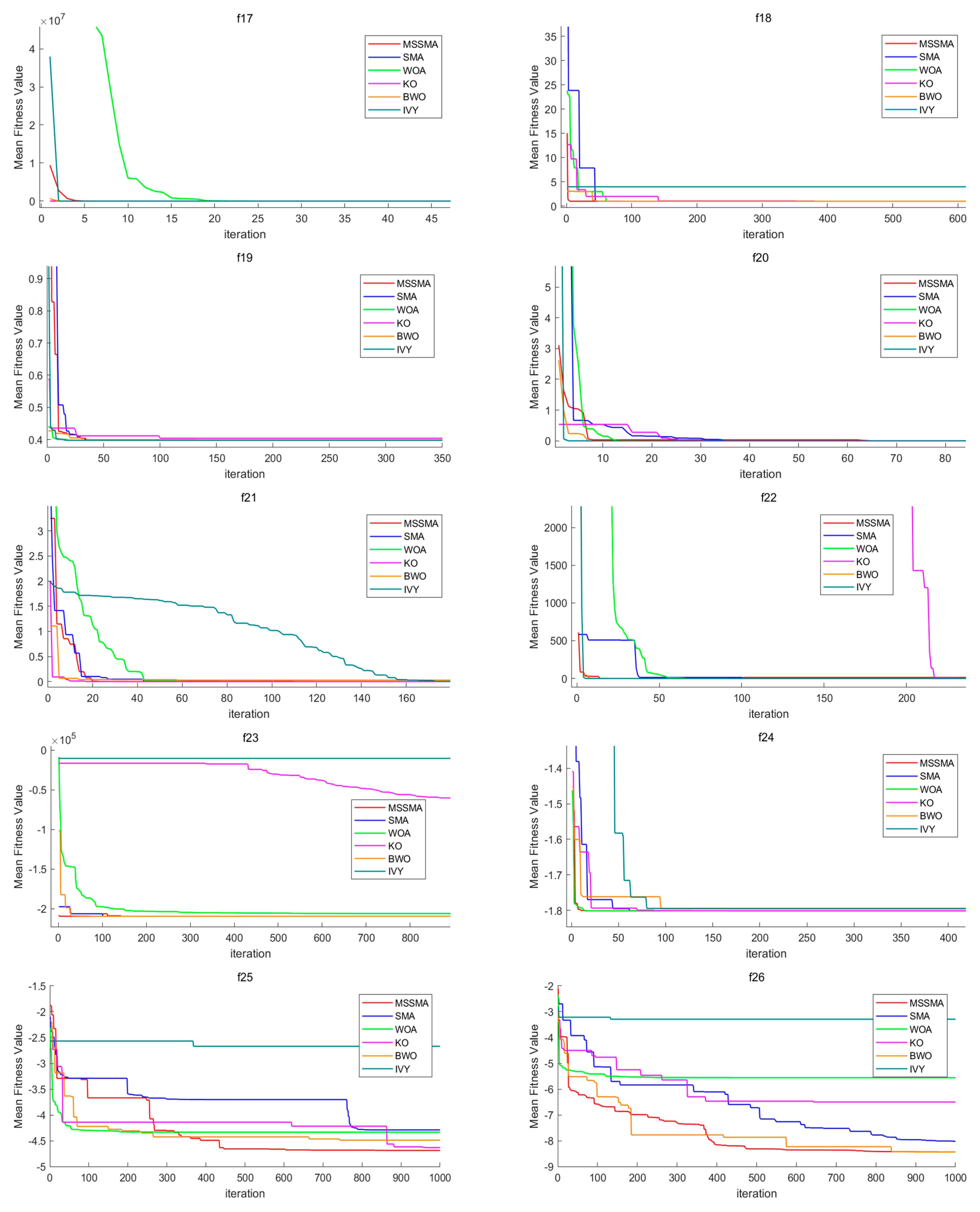
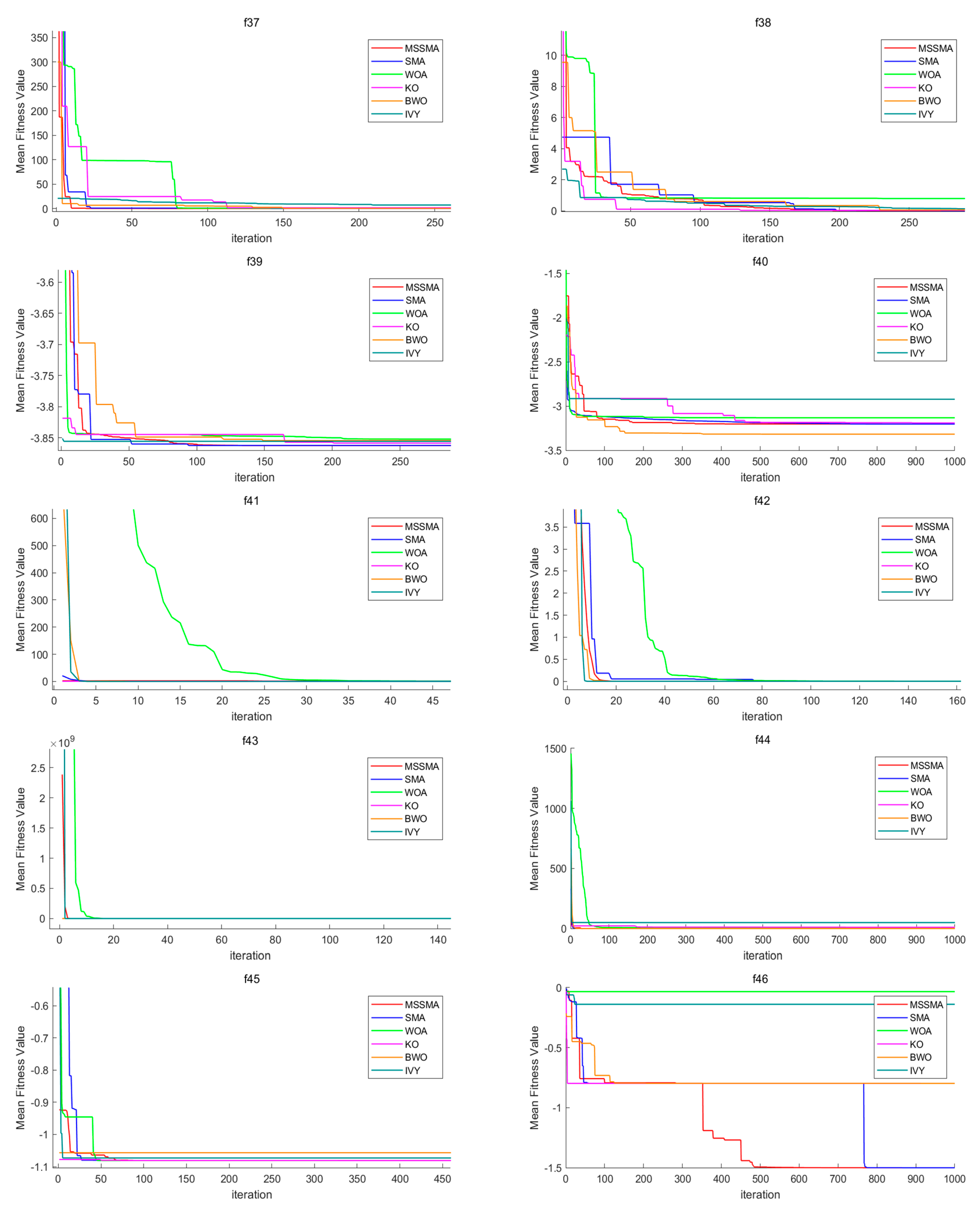
4.3. Comparison of Algorithm Performance

To test the performance of the MSSMA, simulation experiments were conducted for the Whale Optimization Algorithm (WOA) [23], K-mean Optimization Algorithm (KO), Beluga Whale Optimization Algorithm (BWO) [24], Ivy Optimization Algorithm (IVY) [25], and SMA algorithm and MSSMA. To ensure the fairness of the test, the number of populations of all algorithms was 50, the maximum number of iterations was 1000, and each algorithm was tested independently for 30 times, and the mean and variance of each method in different benchmarking functions were calculated.

Table A4. Means and standard deviations of benchmark functions (each winner is shown in bold).

ID	Index	MSSMA	SMA	WOA	KO	BWO	IVY
F1	Mean	−5.00	−5.00	2.46 × 10−187	−4.07	−5.00	−8.00 × 10−1
	Std	0.00	0.00	0.00	3.40 × 10−1	0.00	1.82
F2	Mean	0.00	0.00	4.35 × 10−104	0.00	0.00	0.00
	Std	0.00	0.00	4.79 × 10−206	0.00	0.00	0.00
F3	Mean	0.00	0.00	2.76 × 107	0.00	0.00	0.00
	Std	0.00	0.00	4.76 × 10+13	0.00	0.00	0.00
F4	Mean	0.00	0.00	7.31	0.00	0.00	0.00
	Std	0.00	0.00	6.69	0.00	0.00	0.00
F5	Mean	5.47 × 10−8	3.26 × 10−4	4.13 × 10−6	1.26 × 10−4	3.19 × 10−5	1.86 × 10−5
	Std	3.30 × 10−18	5.45 × 10−8	3.32 × 10−8	1.82 × 10−8	7.03 × 10−10	3.26 × 10−10
F6	Mean	6.75 × 10−10	2.85 × 10−8	0.00	8.46 × 10−7	4.58 × 10−4	6.78 × 10−18
	Std	1.15 × 10−18	2.80 × 10−14	0.00	1.02 × 10−12	4.25 × 10−7	1.00 × 10−33
F7	Mean	−1.00	−9.95 × 10−1	1.95 × 10−4	−1.00	−1.00	−2.16 × 10−1
	Std	1.51 × 10−20	5.76 × 10−4	5.54 × 10−8	1.96 × 10−13	0.00	1.21 × 10−1
F8	Mean	0.00	0.00	−7.89	0.00	0.00	0.00
	Std	0.00	0.00	3.19 × 10−17	0.00	0.00	0.00
F9	Mean	4.81 × 10−7	2.37 × 10−4	0.00	1.39 × 10−1	1.35 × 10−3	1.14
	Std	1.50 × 10−12	2.34 × 10−7	0.00	4.16 × 10−2	2.35 × 10−6	3.01
F10	Mean	−5.00 × 101	−5.00 × 101	2.10 × 10−15	−5.00 × 101	−4.98 × 101	−2.31
	Std	1.11 × 10−18	8.08 × 10−9	4.12 × 10−30	1.48 × 10−7	7.13 × 10−3	1.65 × 101
F11	Mean	−2.10 × 102	−2.10 × 102	2.67 × 10−2	−2.10 × 102	−1.97 × 102	−4.43 × 10−1
	Std	1.92 × 10−9	2.39 × 10−4	2.86 × 10−3	1.66 × 10−4	2.50 × 101	4.99
F12	Mean	0.00	0.00	2.39 × 10−5	0.00	0.00	0.00
	Std	0.00	0.00	3.48 × 10−10	0.00	0.00	0.00
F13	Mean	0.00	0.00	1.21 × 10−2	2.40 × 10−63	0.00	0.00
	Std	0.00	0.00	1.79 × 10−4	1.72 × 10−124	0.00	0.00
F14	Mean	0.00	3.42 × 10−2	1.13 × 10−106	0.00	2.47 × 10−257	0.00
	Std	0.00	1.06 × 10−2	1.56 × 10−211	0.00	0.00	0.00
F15	Mean	0.00	0.00	2.44 × 107	1.20 × 10−302	0.00	0.00
	Std	0.00	0.00	3.70 × 10+13	0.00	0.00	0.00
F16	Mean	2.28 × 10−6	6.85 × 101	4.95 × 102	4.95 × 102	2.68 × 10−3	4.94 × 102
	Std	3.26 × 10−9	1.20 × 104	5.42 × 10−2	6.50 × 10−2	2.00 × 10−4	7.28 × 10−1
F17	Mean	3.46 × 10−4	8.12 × 10−1	6.67 × 10−1	6.67 × 10−1	2.50 × 10−1	6.67 × 10−1
	Std	4.17 × 10−13	8.05 × 10−2	1.90 × 10−9	2.51 × 10−11	1.31 × 10−8	7.74 × 10−10
F18	Mean	9.98 × 10−1	9.98 × 10−1	1.52	9.98 × 10−1	9.98 × 10−1	9.52
	Std	1.86 × 10−26	3.00 × 10−23	3.41	3.98 × 10−24	5.22 × 10−25	1.52 × 101
F19	Mean	3.98 × 10−1	3.98 × 10−1	3.98 × 10−1	3.98 × 10−1	3.99 × 10−1	3.98 × 10−1
	Std	1.10 × 10−18	1.12 × 10−16	9.64 × 10−15	1.65 × 10−7	1.85 × 10−6	3.98 × 10−15
F20	Mean	0.00	0.00	0.00	0.00	0.00	0.00
	Std	0.00	0.00	0.00	0.00	0.00	0.00
F21	Mean	9.58 × 10−11	3.30 × 10−10	3.18 × 10−5	1.00 × 10−6	7.24 × 10−3	1.34 × 10−10
	Std	1.61 × 10−20	5.55 × 10−19	9.44 × 10−10	7.12 × 10−13	2.96 × 10−5	1.42 × 10−19
F22	Mean	0.00	0.00	0.00	0.00	0.00	0.00
	Std	0.00	0.00	0.00	0.00	0.00	0.00
F23	Mean	−1.59 × 105	−2.09 × 105	−1.95 × 105	−6.36 × 104	−2.09 × 105	−1.75 × 104
	Std	1.28 × 10−2	1.18 × 102	4.61 × 108	1.16 × 108	8.76 × 10−22	4.68 × 106
F24	Mean	−1.80	−1.80	−1.80	−1.80	−1.79	−1.69
	Std	2.86 × 10−23	1.67 × 10−17	2.28 × 10−16	1.65 × 10−11	6.16 × 10−5	5.61 × 10−2
F25	Mean	−4.58	−4.39	−3.95	−4.50	−4.55	−2.78
	Std	1.27 × 10−3	8.90 × 10−2	2.95 × 10−1	3.09 × 10−2	4.03 × 10−3	1.89 × 10−1
F26	Mean	−8.57	−8.46	−6.50	−6.78	−8.66	−3.70
	Std	3.42 × 10−2	5.28 × 10−1	7.59 × 10−1	7.92 × 10−1	3.28 × 10−2	3.10 × 10−1
F27	Mean	0.00	0.00	0.00	0.00	0.00	0.00
	Std	0.00	0.00	0.00	0.00	0.00	0.00
F28	Mean	−1.03	−1.03	−1.03	−1.03	−1.03	−9.71 × 10−1
	Std	1.27 × 10−25	9.65 × 10−22	8.25 × 10−23	1.41 × 10−12	5.45 × 10−9	3.55 × 10−2
F29	Mean	0.00	0.00	0.00	0.00	0.00	0.00
	Std	0.00	0.00	0.00	0.00	0.00	0.00
F30	Mean	0.00	0.00	2.59 × 10−17	0.00	0.00	0.00
	Std	0.00	0.00	1.25 × 10−32	0.00	0.00	0.00
F31	Mean	−1.87 × 102	−1.87 × 102	−1.87 × 102	−1.87 × 102	−1.87 × 102	−1.61 × 102
	Std	4.01 × 10−14	1.30 × 10−13	1.75 × 10−10	1.59 × 10−2	4.72 × 10−11	1.02 × 103
F32	Mean	3.00	3.00	3.00	3.00	3.42	3.90
	Std	1.23 × 10−26	2.97 × 10−22	1.12 × 10−11	9.53 × 10−10	1.88 × 10−1	2.43 × 101
F33	Mean	3.08 × 10−4	4.44 × 10−4	5.30 × 10−4	3.36 × 10−4	3.16 × 10−4	1.04 × 10−3
	Std	5.99 × 10−14	2.96 × 10−8	8.88 × 10−8	4.19 × 10−9	1.91 × 10−10	1.34 × 10−5
F34	Mean	−1.02 × 101	−1.02 × 101	−9.73	−1.02 × 101	−1.02 × 101	−2.87
	Std	1.26 × 10−13	2.04 × 10−9	2.66	4.70 × 10−7	3.64 × 10−12	4.09
F35	Mean	−1.04 × 101	−1.04 × 101	−1.00 × 101	−1.04 × 101	−1.04 × 101	−3.66
	Std	4.05 × 10−12	6.36 × 10−9	1.82	2.25 × 10−7	7.32 × 10−12	2.73
F36	Mean	−1.05 × 101	−1.05 × 101	−8.89	−1.05 × 101	−1.05 × 101	−4.01
	Std	4.70 × 10−12	1.82 × 10−9	8.04	2.29 × 10−7	1.92 × 10−11	3.00
F37	Mean	9.26 × 10−2	1.38 × 10−1	3.01	1.04	1.18 × 10−1	3.21 × 10−1
	Std	1.91 × 10−2	3.77 × 10−2	1.13 × 101	9.11 × 10−1	8.40 × 10−3	4.14 × 10−1
F38	Mean	9.57 × 10−4	7.85 × 10−3	9.28 × 10−1	6.61 × 10−2	3.63 × 10−2	1.61 × 10−1
	Std	1.53 × 10−6	7.91 × 10−5	1.32	2.59 × 10−3	7.03 × 10−4	1.09 × 10−1
F39	Mean	−3.86	−3.86	−3.86	−3.86	−3.86	−3.83
	Std	9.69 × 10−22	1.27 × 10−16	3.31 × 10−6	3.20 × 10−9	6.68 × 10−6	1.93 × 10−3
F40	Mean	−3.28	−3.24	−3.26	−3.22	−3.31	−2.74
	Std	2.34 × 10−5	3.07 × 10−3	8.16 × 10−3	3.86 × 10−3	4.56 × 10−4	1.50 × 10−1
F41	Mean	0.00	0.00	0.00	0.00	0.00	0.00
	Std	0.00	0.00	0.00	0.00	0.00	0.00
F42	Mean	3.89 × 10−16	4.44 × 10−16	4.23 × 10−15	4.41 × 10−16	4.16 × 10−16	6.57 × 10−16
	Std	0.00	2.07 × 10−32	7.78 × 10−30	1.07 × 10−28	9.74 × 10−36	3.86 × 10−19
F43	Mean	2.36 × 10−8	4.08 × 10−4	1.49 × 10−2	1.15 × 10−1	1.38 × 10−9	7.85 × 10−2
	Std	4.30 × 10−11	1.05 × 10−6	1.64 × 10−5	2.99 × 10−4	4.75 × 10−8	3.28 × 10−4
F44	Mean	1.07 × 10−3	3.60 × 10−2	4.70	9.64	1.45 × 10−2	4.96 × 101
	Std	5.03 × 10−6	2.28 × 10−3	2.20	7.87	6.12 × 10−5	9.75 × 10−4
F45	Mean	−1.08	−1.08	−1.08	−1.08	−1.06	−9.95 × 10−1
	Std	2.33 × 10−20	4.35 × 10−17	8.42 × 10−6	1.03 × 10−13	3.65 × 10−4	3.00 × 10−2
F46	Mean	−1.40	−1.55 × 10−1	−7.96 × 10−1	−1.28	−1.36	−3.15 × 10−1
	Std	5.40 × 10−3	9.16 × 10−2	8.55 × 10−2	4.83 × 10−3	3.92 × 10−2	2.32 × 10−2
F47	Mean	−9.40 × 10−1	−1.37 × 10−3	−2.52 × 10−1	−1.07 × 10−1	−6.27 × 10−1	−2.42 × 10−2
	Std	5.57 × 10−5	3.32 × 10−4	2.75 × 10−2	1.91 × 10−1	3.01 × 10−2	5.90 × 10−3
F48	Mean	2.85 × 10−9	1.46 × 10−8	3.53 × 10−9	1.13 × 10−1	1.28 × 101	4.70 × 101
	Std	3.33 × 10−17	3.24 × 10−16	3.24 × 10−17	1.17 × 10−2	1.87 × 102	3.20 × 104
F49	Mean	1.04 × 102	2.82 × 102	4.08 × 102	6.79 × 102	8.91 × 102	9.92 × 102
	Std	2.45 × 105	5.67 × 105	6.34 × 105	6.96 × 101	5.06 × 103	2.96 × 106
F50	Mean	3.83 × 103	5.17 × 103	9.67 × 103	2.15 × 103	3.61 × 103	4.09 × 103
	Std	4.86 × 106	6.29 × 106	1.61 × 108	1.05 × 107	6.90 × 105	3.05 × 107

shows the experimental data of the six algorithms on a test set consisting of 50 benchmark test functions, with the best results highlighted in bold.

To further analyze the statistical significance of the selected improvements, the Friedman test and the Wilcoxon signed-rank test with a significant level p-value of 0.05 were used. The other five algorithms were compared with the MSSMA to obtain the p-value in the last row of

Table 3. The experimental results of six algorithms on Friedman and Wilcoxon signed-rank test.

ID	MSSMA	SMA	WOA	KO	BWO	IVY
(W|T|L)	(43|7|0)	(14|31|5)	(7|32|11)	(13|35|2)	(7|40|3)	(14|16|20)
Ave	1.86	2.88	3.22	3.94	4.58	4.52
Rank	1	2	3	4	6	5
p-value	-	0.0159	9.7 × 10−6	0.0013	0.0242	0.003

(the MSSMA was not compared with itself, so the corresponding cell is “-”). If the p-value was less than 0.05, it meant that there was a significant difference between the two algorithms in terms of performance; on the contrary, it was considered that there was no significant difference between the two algorithms. The results show that all p-values were less than 0.05, which indicates that the performance of the MSSMA is significantly different from those of the other algorithms and statistically verifies the superiority and reliability of the MSSMA.

Table 3 shows the results of the six algorithms on the test function. From the (W|T|L) and Friedman average ranking results in the table, it can be seen that the MSSMA significantly outperformed the other five algorithms compared on most of the test functions. The specific analysis is as follows.

From Table 3, we can see that the MSSMA achieved 14 best results on seventeen single-peak functions, 29 best results on thirty-three multi-peak functions, and only slightly worse test results on seven functions. Specifically, the MSSMA achieved the second-best results on functions f7, f9, f26, f40, and f43 and the third-best results on functions f6 and f50. In addition, the improved algorithm outperformed SMA on all 50 functions tested, reflecting the good results of the improved strategy. The convergence curve of the algorithm is shown in Figure A1.

The MSSMA performed much better than other algorithms on UN (single-peak non-separable) and US (single-peak separable) functions, which shows that the MSSMA has better exploration capability. It can also be seen that the MSSMA performed better than other algorithms on MS (multimodal separable) and MN (multimodal non-separable) functions, indicating that the MSSMA can better avoid local optima and has better exploration capability. In summary, the solution accuracy and stability of the MSSMA are generally better than those of the other five algorithms.

4.4. Collaborative Multi-UAV Path Planning

Collaborative multi-UAV path planning has important applications in several fields. In search and rescue, multiple drones can work together to cover large areas, quickly locate survivors, and avoid obstacles while avoiding repeated searches by sharing information in real time [26]. In agricultural monitoring, drones can efficiently collect farmland data, optimize paths to cover the entire area, and avoid collisions, improving monitoring efficiency [27]. In logistics distribution, multiple UAVs collaborate to perform package delivery tasks, dynamically adjusting paths to cope with obstacles and traffic changes in urban environments to ensure delivery accuracy and timeliness.

The main methods for collaborative multi-UAV path planning include centralized planning, distributed planning, and population intelligence algorithms [28,29]. Centralized planning assigns tasks and paths to all UAVs by a central controller, which is suitable for small teams but has high computational complexity; distributed planning relies on the autonomous decision making of each UAV, which is suitable for large teams but requires an efficient communication mechanism; swarm intelligence algorithms such as Particle Swarm Optimization (PSO) and Ant Colony Algorithms (ACOs) solve the multi-objective optimization problem by simulating natural behaviors but may face the convergence challenges of slow speed.

The difficulties in cooperative multi-UAV path planning are mainly focused on environmental complexity, dynamic obstacles, and communication constraints [30]. Complex 3D environments require path planning algorithms that can efficiently handle obstacles and terrain changes; dynamic obstacles, such as moving vehicles or other UAVs, require real-time path adjustments to avoid collisions; and communication constraints can affect the efficiency of UAV collaboration, especially in large teams or long-distance missions. In addition, multi-objective optimization (e.g., of path length, energy consumption, and mission completion time) adds to the complexity of the problem.

The flight paths of UAVs are affected by many factors, and in this paper, we construct path planning evaluation functions in terms of path length, deflection angle size, and flight threat conditions.

Usually, when the UAV maintains a fixed speed during flight, f_L can be equivalently expressed as a fixed proportion of the flight path length, as shown in Equation (23) [31].

$$\begin{array}{c}{f}_L={\sum }_{i=1}^n{l}_i\end{array}$$

(23)

Here, l_i is the distance from the ith path point Li to the next path point Li + 1.

The flight altitude of the UAV is limited by the function f_H as shown in Equation (24):

$$\begin{array}{c}{f}_H={\sum }_{i=1}^n{h}_i\end{array}$$

(24)

Here, the altitude penalty function h_i is shown in Equation (25).

$$\begin{array}{c}hi=\left\{\begin{array}{c}\left(z_i-H_{max}\right) ,{z_i>H}_{max} \\ 0 , H_{min}\le z_i\le H_{max}\\ \left(H_{min}-z_i\right) ,{z_i<H}_{min} \end{array}\right.\end{array}$$

(25)

Here, z_i is the flight altitude of the ith path point, and H_max and H_min are the maximum and minimum flight altitudes of the UAV, respectively.

To further test the performance of the algorithm, a battlefield environment with radar, missiles, and other threats is simulated as follows [32]. Here, the threat probability from radar to UAV can be approximated as follows:

$$\begin{array}{c}P\left(d_R\right)=\left\{\begin{array}{c} 0 , d_R>d_{R_{max}} \\ {\displaystyle \raisebox{1ex}{$1$}\!\left/ \!\raisebox{-1ex}{$d_R^4$}\right.} , d_{R_{min}}\le d_R\le d_{R_{max}} \\ 1 ,d_R<d_{R_{min}} \end{array}\right.\end{array}$$

(26)

Here, d_R is the distance between the UAV and the radar, and the fractions D_Rmax and D_Rmin are the maximum detection radius and effective detection radius of the radar.

$$\begin{array}{c}P\left(d_M\right)=\left\{\begin{array}{c} 0 , d_M>d_{M_{max}} \\ {\displaystyle \raisebox{1ex}{$1$}\!\left/ \!\raisebox{-1ex}{$d_M$}\right.} , d_{M_{min}}\le d_M\le d_{M_{max}} \\ 1 ,d_M<d_{M_{min}} \end{array}\right.\end{array}$$

(27)

Here, d_M is the distance between the UAV and the missile, and D_Mmax and D_Mmin are the maximum kill radius and effective kill radius of the missile.

$$\begin{array}{c}P\left(d_A\right)=\left\{\begin{array}{c} 0 , d_A>d_{A_{max}} \\ {\displaystyle \raisebox{1ex}{$1$}\!\left/ \!\raisebox{-1ex}{$d_A$}\right.} , d_{A_{min}}\le d_A\le d_{A_{max}} \\ 1 ,d_A<d_{A_{min}} \end{array}\right.\end{array}$$

(28)

Here, d_A is the distance between the UAV and the anti-aircraft gun, and the ratios of D_Amax and D_Amin are the maximum kill radius and effective kill radius of the anti-aircraft gun.

$$\begin{array}{c}P\left(d_C\right)=\left\{\begin{array}{c} 0 , d_C>d_{C_{max}} \\ {\displaystyle \raisebox{1ex}{$1$}\!\left/ \!\raisebox{-1ex}{$d_C$}\right.} , d_{C_{min}}\le d_C\le d_{C_{max}} \\ 1 ,d_C<d_{C_{min}} \end{array}\right.\end{array}$$

(29)

Here, d_C is the distance between the UAV and the atmosphere, and the ratios of D_Cmax and D_Cmin are the maximum kill radius and effective kill radius of the atmosphere.

Then, the threat function f_B is determined as shown in Equation (30).

$$\begin{array}{c}{f}_B=r\times P\left(d_R\right)+m\times P\left(d_M\right)+a\times P\left(d_A\right)+c\times P\left(d_C\right)\end{array}$$

(30)

In the formula, r, m, a, and c are the influence factors of the radar, missile, artillery, and atmosphere on the threat probability of the UAV, respectively.

Zhou et al. set up a method of defining the time co-constraints with fewer steps and less computation [33], i.e., they set up the command time for the UAV to reach the end point and the time range to solve for its arrival at the target end point and determine the time cost function by judging the relationship between the two as shown in Equation (31). Assuming that the command time for the UAV to reach the target endpoint is tc, the shortest time $t_{min}^i$ and the longest time $t_{max}^i$ for the UAV to reach the target endpoint are derived based on its speed range and trajectory length.

$$\begin{array}{c}f\left(t_i\right)=\left\{\begin{array}{c} 0 , t_{min}^i\le t_c\le t_{max}^i \\ \left|t_i-t_c\right| , t_{min}^i>t_c or { t}_c>t_{max}^i\end{array}\right.\end{array}$$

(31)

Here, t_i is the actual time for the ith UAV to reach the target endpoint.

Summing the time cost function yields the total time cost function f_T as shown in Equation (32).

$$\begin{array}{c}{f}_T={\sum }_{i=1}^n{f(t}_i)\end{array}$$

(32)

Based on the above, the following evaluation function for path planning is derived:

$$\begin{array}{c}f4={\omega }_1\times f_L+{\omega }_2\times f_H+{\omega }_3\times f_B+{\omega }_4\times f_T\end{array}$$

(33)

Here, w1, w2, w3, and w4 are the weights of the functions f_L, f_H, f_B, and f_T, respectively, and satisfy the constraint ω1 + ω2 + ω3 + ω4 = 1.

Figure 5: Threat areas and pathways planned by MSSMA. illustrates the established threat areas and the path planned by MSSMA.

In order to test the performance of the MSSMA on collaborative multi-UAV path planning applications, the Whale Optimization Algorithm (WOA), K-mean Optimization Algorithm (KO), Beluga Optimization Algorithm (BWO), Ivy Optimization Algorithm (IVY), and SMA and MSSMA collaborative multi-UAV path planning algorithms were used. To ensure the fairness of the test, the number of populations of all algorithms was 50, the maximum number of iterations was 100, and each algorithm was tested independently 30 times, and the minimum, mean, and variance of each method were calculated, and the results are shown in

Table 4. Statistical results of a collaborative multi-UAV 3D path plan.

ID	Minimum Cost	Mean Cost	Var
MSSMA	53.641	103.123	74.996
SMA	127.708	143.431	106.813
WOA	183.296	247.842	245.518
KO	136.166	196.649	305.482
BWO	2350.998	2421.506	1558.914
IVY	213.893	265.483	81.260

. The minimum cost, mean cost, and variance of all the algorithms were significantly higher compared to those of the MSSMA. This indicates that MSSMA performs better in terms of optimization stability during path planning.

5. Conclusions

The MSSMA uses four different strategies to improve the SMA algorithm: (1) using chaotic mapping and inverse learning to generate a better initial population and improve the convergence accuracy; (2) proposing a balancing factor B based on the fitness value order, and according to B, dividing the population into two parts that are searched globally and locally (this ensures that the individuals with poor fitness values are searched globally in the early stage of iteration, and locally around the individuals’ optima in the later stage of iteration, which better maintains the balance between exploration and exploitation of the algorithm); (3) introducing the improved Lévy flight strategy, which performs random searches around the individuals of the initial population that are obtained to be more optimal, and has a better chance of discovering the optimal solution than the random generation strategy; and (4) using the elite tangent search strategy to perform larger-scale local searches around the individual when it falls into local optimality, which accelerates the convergence of the algorithm and improves the ability to jump out of local optimality.

Compared with the other five algorithms such as SMA, the MSSMA achieved better experimental results in a test set of 50 benchmark test functions, which proves the effectiveness of the improved strategy. In addition, the MSSMA performed better in terms of the stability of planning path optimization with better paths in collaborative multi-UAV path planning, which is expected to have a wide range of applications in collaborative multi-UAV path planning problems.

References

1. Shadravan, S.; Naji, H.R.; Bardsiri, V.K. The Sailfish Optimizer: A novel nature-inspired metaheuristic algorithm for solving constrained engineering optimization problems. Eng. Appl. Artif. Intell. 2019, 80, 20–34. [Google Scholar] [CrossRef]
2. Wu, G. Across neighborhood search for numerical optimization. Inf. Sci. 2016, 329, 597–618. [Google Scholar] [CrossRef]
3. Chou, J.-S.; Truong, D.-N. A novel metaheuristic optimizer inspired by behavior of jellyfish in ocean. Expert Syst. Appl. 2021, 165, 113702. [Google Scholar] [CrossRef]
4. Wu, J.; Zhang, Z.; Yang, Y.; Zhang, P.; Fan, D. Time-optimal trajectory planning for robotic arms based on an improved tuna swarm algorithm. Comput. Integr. Manuf. Syst. 2024, 30, 4292–4301. [Google Scholar]
5. Li, S.; Chen, H.; Wang, M.; Heidari, A.A.; Chen, Y.; Pan, Z. Slime mould algorithm: A new method for stochastic optimization. Future Gener. Comput. Syst. 2020, 111, 300–323. [Google Scholar] [CrossRef]
6. Jia, H.; Liu, Y.; Liu, Q.; Wang, S.; Zheng, R. A hybrid optimization algorithm combining slime mould and arithmetic with random opposition-based learning. J. Comput. Sci. Explor. 2022, 16, 1182–1192. [Google Scholar]
7. Guo, Y.; Liu, S.; Zhang, L.; Huang, Q. An improved slime mould algorithm with elite opposition-based learning and quadratic interpolation. Comput. Appl. Res. 2021, 38, 3651–3656. [Google Scholar] [CrossRef]
8. Huang, H.; Gao, Y.; Ru, F.; Yang, L.; Wang, H. Three-dimensional path planning for UAVs based on adaptive slime mould algorithm optimization. J. Shanghai Jiao Tong Univ. 2023, 57, 1282–1291. [Google Scholar] [CrossRef]
9. Chen, L.F.; Cao, K.X.; Zhang, S.P.; Bai, H.R.; Han, Y.; Dai, Q. Recent advances in swarm intelligent optimization algorithms. Comput. Eng. Appl. 2024, 60, 46–67. [Google Scholar] [CrossRef]
10. Maaranen, H.; Miettinen, K.; Mäkelä, M.M. Quasi-random initial population for genetic algorithms. Comput. Math. Appl. 2004, 47, 1885–1895. [Google Scholar] [CrossRef]
11. Poles, S.; Fu, Y.; Rigoni, E. The effect of initial population sampling on the convergence of multi-objective genetic algorithms. In Multiobjective Programming and Goal Programming: Theoretical Results and Practical Applications; Springer: Berlin/Heidelberg, Germany, 2009; pp. 123–133. [Google Scholar]
12. Ibada Ali, J.; Tüű-Szabó, B.; Kóczy, T.L. Effect of the initial population construction on the DBMEA algorithm searching for the optimal solution of the traveling salesman problem. Infocommunications J. 2022, 14, 72–78. [Google Scholar] [CrossRef]
13. Li, J.W.; Cheng, Y.M.; Chen, K.Z. Chaotic particle swarm optimization algorithm based on adaptive inertia weight. In Proceedings of the 26th Chinese Control and Decision Conference (2014 CCDC), Changsha, China, 31 May–2 June 2014; pp. 1310–1315. [Google Scholar]
14. Hui, L.C.; Chen, X.L.; Meng, Z.B. An improved sparrow search algorithm with multi-strategy hybridization. Comput. Eng. Appl. 2022, 58, 71–83. [Google Scholar]
15. Ewees, A.A.; Abd Elaziz, M.; Houssein, E.H. Improved grasshopper optimization algorithm using opposition-based learning. Expert Syst. Appl. 2018, 112, 156–172. [Google Scholar] [CrossRef]
16. Zhou, X.Y.; Yin, Z.Y.; Gao, W.F.; Tan, G.S.; Yi, Y.G. An adaptive multi-neighborhood artificial bee colony algorithm based on reinforcement learning. J. Comput. 2024, 47, 1521–1546. [Google Scholar]
17. Wu, F.; Chen, K.; Wang, W.L. A review of computational intelligence based on parallel computing. J. Zhejiang Univ. (Eng. Ed.) 2025, 59, 27–38. [Google Scholar]
18. Minh, H.L.; Sang-To, T.; Wahab, M.A.; Cuong-Le, T. A new metaheuristic optimization based on K-means clustering algorithm and its application to structural damage identification. Knowl. -Based Syst. 2022, 251, 109189. [Google Scholar] [CrossRef]
19. Layeb, A. Tangent search algorithm for solving optimization problems. Neural Comput. Appl. 2022, 34, 8853–8884. [Google Scholar] [CrossRef]
20. Tao, X.M.; Guo, W.J.; Li, X.K.; Chen, W.; Wu, Y.K. Dimensionally reset multiple swarm particle swarm algorithm based on density peaks. J. Softw. 2023, 34, 1850–1869. [Google Scholar] [CrossRef]
21. Chen, Z.; Damian, Z.; Ziyun, X. A new species of the genus Pseudococcus (Coleoptera, Staphylinidae) from China. A symbiotic nonuniform Gaussian variational bottle sea squirt swarm algorithm for multisubgroups. J. Autom. 2011, 48, 1307–1317. [Google Scholar] [CrossRef]
22. Zhao, W.; Wang, L.; Mirjalili, S. Artificial hummingbird algorithm: A new bio-inspired optimizer with its engineering applications. Comput. Methods Appl. Mech. Eng. 2022, 388, 114194. [Google Scholar] [CrossRef]
23. Mirjalili, S.; Lewis, A. The whale optimization algorithm. Adv. Eng. Softw. 2016, 95, 51–67. [Google Scholar] [CrossRef]
24. Zhong, C.; Li, G.; Meng, Z. Beluga whale optimization: A novel nature-inspired metaheuristic algorithm. Knowl.-Based Syst. 2022, 251, 109215. [Google Scholar] [CrossRef]
25. Ghasemi, M.; Zare, M.; Trojovský, P.; Rao, R.V.; Trojovská, E.; Kandasamy, V. Optimization based on the smart behavior of plants with its engineering applications: Ivy algorithm. Knowl.-Based Syst. 2024, 295, 111850. [Google Scholar] [CrossRef]
26. Michelon, G.K.; Assunção, W.K.; Grünbacher, P.; Egyed, A. Analysis and propagation of feature revisions in preprocessor-based software product lines. In Proceedings of the 2023 IEEE International Conference on Software Analysis, Evolution and Reengineering (SANER), Taipa, Macao, 21–24 March 2023; pp. 284–295. [Google Scholar]
27. Schlosser, A.D.; Szabó, G.; Bertalan, L.; Varga, Z.; Enyedi, P.; Szabó, S. Building Extraction Using Orthophotos and Dense Point Cloud Derived from Visual Band Aerial Imagery Based on Machine Learning and Segmentation. Remote Sens. 2020, 12, 2397. [Google Scholar] [CrossRef]
28. Shan, J.R. Research on Multi-AUV Task Assignment and Path Planning Based on Swarm Intelligence Algorithm. Master’s Thesis, Jilin University, Changchun, China, 2024. Available online: https://kns.cnki.net/kcms2/article/abstract?v=b41E60TuiN92yX80tKT_USqnbcSNTnxPQKhL4fFkW-XNZDWl1InNX-8Dcn9rpiwkepQv1v6478hR0Z6BX8foFcZYjotIkicM5EwiERYMp3b901hmdbSBul97a6VlBiwCki07dsMcghujyaacLzn4Uh8y0WGPTiPNv7OMzT7fHElTFXPJ2HPuvoPwch0OaM5cNNaUZ3GmvIuJbpDNVQlMNA==&uniplatform=NZKPT (accessed on 10 March 2025).
29. Peng, H.; Zhang, J.; Li, H.; Hu, J. Cooperative UAV mission planning based on improved wolfpack algorithm. Comput. Eng. 2024, 50, 69–79. [Google Scholar] [CrossRef]
30. Wang, F.; Zhang, H.; Han, M.; Xing, L.N. Co-evolutionary mixed-variable multi-objective particle swarm optimization algorithm based on co-evolution for solving UAV cooperative multi-tasking problem. J. Comput. 2021, 44, 1967–1983. [Google Scholar]
31. Liu, C.-A.; Wang, X.; Liu, C.; Wu, H. Three-dimensional trajectory planning for unmanned aerial vehicles based on improved gray wolf optimization algorithm. J. Huazhong Univ. Sci. Technol. (Nat. Sci. Ed.) 2017, 45, 38–42. [Google Scholar] [CrossRef]
32. Hu, Z.; Zhao, M.; Yao, M.; Li, K.H.; Wu, R. An improved ant algorithm for UAV multi-target 3D trajectory planning. J. Shenyang Univ. Technol. 2011, 33, 570–575. [Google Scholar]
33. Zhou, R.; Huang, C.Q.; Wei, Z.L.; Zhao, K.X. Application of MP-GWO algorithm in multi-UCAV cooperative trajectory planning. J. Air Force Eng. Univ. (Nat. Sci. Ed.) 2017, 18, 24–29. [Google Scholar]
Figure 1. Possible locations in (a) 2 dimensions and (b) 3 dimensions [5].
Applsci 15 05456 g001
Figure 2. Assessment of fitness [5].
Applsci 15 05456 g002
Figure 3. Sine chaotic mapping bifurcation diagram.
Applsci 15 05456 g003
Figure 4. Distribution of step size Levy_S in two dimensions for different β-parameters.
Applsci 15 05456 g004