Article

Improved War Strategy Optimization with Extreme Learning Machine for Health Data Classification

by
İbrahim Berkan Aydilek
1,*,
Arzu Uslu
2 and
Cengiz Kına
1
1
Department of Computer Engineering, Faculty of Engineering, Osmanbey Campus, Harran University, Sanliurfa 63100, Turkey
2
Department of Internal Medicine Nursing, Faculty of Health Sciences, Osmanbey Campus, Harran University, Sanliurfa 63100, Turkey
*
Author to whom correspondence should be addressed.
Appl. Sci. 2025, 15(10), 5435; https://doi.org/10.3390/app15105435
Submission received: 26 March 2025 / Revised: 9 May 2025 / Accepted: 12 May 2025 / Published: 13 May 2025
(This article belongs to the Special Issue Intelligent Computing Systems and Their Applications)

Abstract

:
Classification of diseases is of great importance for early diagnosis and effective treatment processes. However, etiological factors of some common diseases complicate the classification process. Therefore, classification of health datasets by processing them with artificial neural networks can play an important role in the diagnosis and follow-up of diseases. In this study, disease classification performance was examined by using Extreme Learning Machine (ELM), one of the machine learning methods, and an opposition-based WSO algorithm with a random opposite-based learning strategy is proposed. Common health datasets: Breast, Bupa, Dermatology, Diabetes, Hepatitis, Lymphography, Parkinsons, SAheart, SPECTF, Vertebral, and WDBC are used in the experimental studies. Performance evaluation was made by accuracy, precision, sensitivity, specificity, and F1 score metrics. The proposed IWSO-based ELM model has demonstrated better classification success compared to the ALO, DA, PSO, GWO, WSO, OWSO metaheuristics, and LightGBM, XGBoost, SVM, Neural Network (MLP), CNN machine and deep learning methods. In the Wilcoxon test, it was determined that IWSO was p < 0.05 when compared to other algorithms. In the Friedman test, it was determined that IWSO was first in the ranking of success compared to other algorithms. The results reveal that the IWSO approach developed with ELM is an effective method for the accurate diagnosis of common diseases.

1. Introduction

With the development of technology, data in the field of health is becoming widespread. Improvements are made in patient diagnosis using health data with artificial intelligence algorithms. Models are created to be used in predicting, treating, monitoring, and managing a health-related disease or medical condition. Methods consisting of the processing and training processes of many data, including patients’ medical records, medical images, data received from sensors, and simultaneous verbal data, are used. As a result of all this, patients are provided with individualized treatment and care. Thus, the cost of treatment is reduced, and diseases are diagnosed early and accurately. There are improvements in patient results in a short time. It provides the opportunity to follow and monitor the patient simultaneously. It predicts the severity of the disease, death, and survival of the patients and determines the risky patients [1]
Disease diagnosis classifications in the field of health are made according to the ICD (International Classification of Diseases) guide [2]. Although this classification guide, which defines disease and health-related problems, is instructive, it can be confusing or take time due to its excessive detail. While making the correct diagnosis, the use of artificial intelligence-supported applications makes things much easier and minimizes errors. Correct classification of diseases such as heart diseases, liver diseases, breast cancer, diabetes, which are especially common, in a short time prevents possible disabilities and diseases [3]. It is essential to make successful classifications using artificial intelligence algorithms in important issues such as human life and common diseases. ELM, one of the machine learning methods, stands out compared to ANN and DNN due to its fast convergence capability compared to other algorithms and its ability to be trained on low-dimensional data [4].
ELM (Extreme Learning Machine), which is one of the feedforward neural networks, is a frequently preferred learning algorithm due to its fast and precise classification capability. In ELM, the fact that the input weights are random, that it works faster, that it can generalize faster, and that different activation functions (sigmoid, hardlim, sine, etc.) can be used to provide an advantage by performing better. However, overfitting (overlearning), poor determination of initial weights, incorrect activation function, and hidden layer neuron number choices can negatively affect ELM results by making the performance sensitive [4].
Optimization algorithms are used to improve the classification success of complex, difficult-to-solve, and time-consuming problems. Optimization algorithms are frequently used to solve problems that require long-term solutions in large solution spaces in a reasonable time [5]. In nonparametric data, it is used to determine neighborhood relationships. This method provides optimization by analyzing the proximity of certain data points to each other.
In ELM, better learning occurs through optimization of parameters with metaheuristic algorithms. As a result, the diagnosis of the disease can be made successfully by making a more accurate classification. Studies on the health data of common diseases in the world are included in detail in Section 2. The WSO (War Strategy Optimization) algorithm was proposed by Ayyarao et al. based on war strategy [6]. This algorithm can provide more accurate results by making the process of finding solutions more efficient, especially in complex optimization problems.
The opposite-based learning strategy is an optimization that provides faster convergence by exploring the opposite solutions of a candidate solution in the search space [7]. Random opposite-based learning strategy can be used to achieve more successful classification of health data with optimization algorithms for more successful exploration of the search space. While different solution candidates are intuitively sought in the optimization process, it is aimed to achieve global results with opposite-based candidates. It is very important to achieve high classification success on data that is important for human life, such as health. In this study, it is to optimize ELM parameters with a random opposite-based learning strategy developed and successful experimental results on health data.
Our main motivation in this article is to optimize the input layer weight and bias values, which are disadvantages of the ELM training process. ELM is a reliable classifier and has been used successfully in many areas, as stated in Section 2. For this purpose, the recently developed WSO is used to achieve optimization and perform high-accuracy classification with ELM. In order to achieve a correct balance between the exploration and exploitation ability of WSO, increase diversity, and escape from the local optimums, opposition-based learning (OBL) was integrated with a random strategy.
The structure of the paper is organized as follows: In Section 2, a comprehensive review of the relevant literature is presented. Section 3 outlines the structure and operation of the Extreme Learning Machine (ELM) algorithm, while Section 4 and Section 5 provide detailed descriptions of the War Strategy Optimization (WSO) algorithm and the opposition-based learning (OBL) strategy, respectively. The proposed IWSO algorithm is introduced in Section 6. Section 7 presents the performance evaluation, and Section 8 describes the datasets used in the study. Section 9 discusses the tested and benchmarked methods. The results and their interpretation are given in Section 10, followed by conclusions in Section 11.

2. Literature Review

In recent years, the classification of medical datasets has been significantly enhanced through the integration of machine learning algorithms with optimization techniques. Particularly, Extreme Learning Machine (ELM), due to its fast training speed and high generalization capability, has been widely adopted in various health-related classification problems. However, ELM’s sensitivity to parameter initialization has necessitated the use of metaheuristic optimization methods to improve its performance.
Various algorithms have been employed in the literature to enhance ELM-based classification for specific datasets. For the Breast Cancer dataset, high accuracy rates have been reported using different approaches: Flower Pollination Algorithm (FPA) and Gray Wolf Optimization (GWO) achieved 97.81% [8]; Radial Basis Function (RFFs) and Radial Basis Function Neural Networks-ELM-Genetic Algorithm (RBFNN-ELM-GA) attained 97.38% [9]; and Differential Evolution (DE) reached 98.74% [10]. For the Bupa dataset, accuracies include 88.90% for Hybrid Activation-based ELM (HAELM) [11], 76.75% for Artificial Bee Colony (ABC) [12], and 88.36% for ELM [13].
In the classification of the Dermatology dataset, the combination of Factor Analysis (FA) with ELM achieved 100% accuracy [14], while Principal Component Analysis-Kernel ELM (PCA-KELM) reached 95.60% [15]. In the Diabetes dataset, accuracy rates of 78.62% with Particle Swarm Algorithm (PSO) [8], 77.61% with RBF and RBFNN-ELM-GA [9], and 79.69% with ELM [10] have been reported. For the Hepatitis dataset, RBFNN-ELM-GA achieved 87.10% accuracy [9], ELM yielded 63.54% [15], and Improved Cuckoo Search-Based ELM (ICSELM) achieved 100% [13]. For the Lymphography dataset, the NEURO-FUZZY algorithm attained an accuracy of 89.19% [15].
Several notable studies have demonstrated the impact of optimization strategies on ELM and related classifiers. Al Bataineh and Manacek proposed a PSO-optimized MLP model for heart disease prediction, achieving 84.61% accuracy on the Cleveland dataset, outperforming several traditional classifiers such as SVM and Random Forest [16]. Albadr et al. developed a GWO-ELM model for the detection of diabetic retinopathy using HOG and PCA, reporting up to 99.47% accuracy on APTOS-2019 and IDRiD datasets [17].
Chen et al. [18] proposed a lightweight fuzzy SZGWO-ELM neural network model that combines an Extreme Learning Machine (ELM) with an improved Grey Wolf Optimization (GWO) algorithm. The SZGWO-ELM model was evaluated on five UCI medical datasets and achieved high performance with accuracy (96.08%), sensitivity (94.14%), specificity (99.26%), and precision (99.52%).
Bacanin et al. (2024) [19] proposed a method to enhance the performance of Extreme Learning Machine (ELM) classifiers by tuning both the hidden layer neuron count and the initial weights/biases using an improved Firefly Algorithm (FA), named Group Search Firefly Algorithm (GSFA). The proposed ELM-GSFA model was evaluated on 16 benchmark datasets, including both real and synthetic medical datasets, and outperformed nine other metaheuristic-tuned ELM models. Notably, it achieved 84.85% accuracy on the Diabetes dataset, 98.7% on the heart disease dataset, and 83.7% on the Cardiotocography-10 dataset. The results demonstrated that GSFA significantly improves classification accuracy and robustness, particularly on imbalanced and multiclass datasets.
Lahoura et al. (2021) [20] proposed a cloud-based framework for breast cancer diagnosis that leverages the Extreme Learning Machine (ELM) classifier in combination with gain ratio-based feature selection. Using the Wisconsin Diagnostic Breast Cancer (WDBC) dataset, the cloud-based ELM achieved high accuracy (98.68%), recall (91.30%), precision (90.54%), and F1 score (81.29%), highlighting its potential as a rapid and scalable diagnostic tool for remote healthcare applications.
Although the name Random Opposition-Based Learning (ROBL) has previously appeared in the literature [21,22,23], the strategy proposed in this study differs in its mathematical formulation. This differs from previously proposed ROBL variants, which often use uniform random distributions over fixed search space boundaries. Therefore, as we know, the ROBL mechanism employed in this paper is considered a novel variant, tailored specifically for enhancing the exploratory capabilities of the WSO.
Collectively, these studies underline the effectiveness of combining ELM with advanced optimization techniques, particularly in medical diagnosis applications. The proposed IWSO-ELM approach contributes to this growing body of research by offering a novel configuration that has not yet been explored in the literature and demonstrating competitive classification performance across multiple challenging health datasets.
The current accuracy results of many metaheuristic algorithms used in ELM learning for health data (Breast, Bupa, Dermatology, Diabetes, Hepatitis, Lymphography, Parkinsons, SAheart, SPECTF, Vertebral, WDBC) in the literature are shown in Appendix A. Table A1 and the explanations of the algorithms used are shown at the bottom of the table. When these data are examined, it is seen that some of the accuracy, precision, sensitivity, specificity, and F1 score accuracy parameters were evaluated in disease classification. As far as we know, the ELM and WSO algorithms were not used together in these datasets.

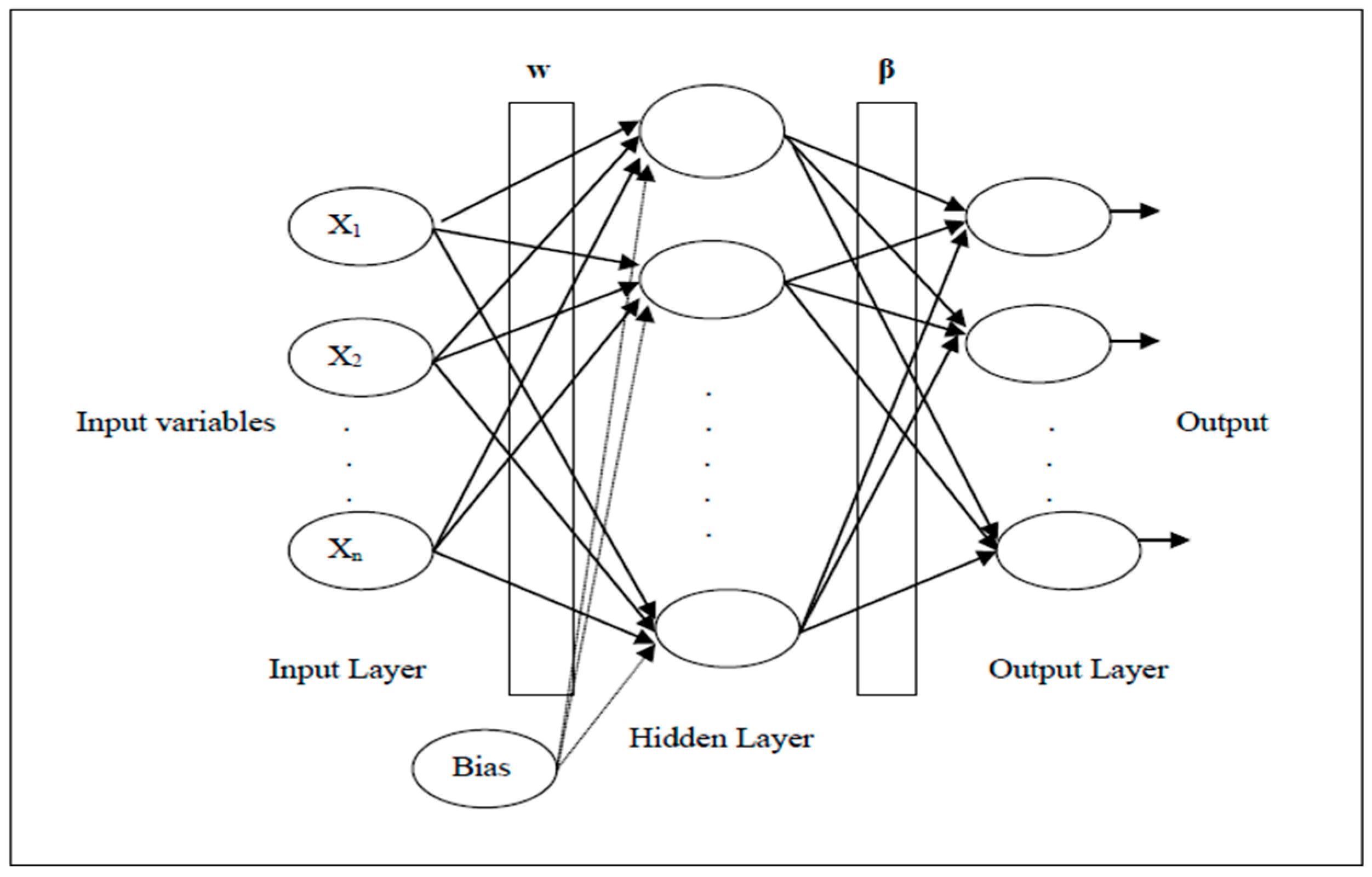
3. Extreme Learning Machine (ELM)

ELM is a feedforward neural network with random input layer weights with a single hidden layer [24]. In ELM, a linear method is used to calculate the weights between the hidden layer and the output layer (Figure 1). In this linear method, the generalized inverse matrix, which is the Moore–Penrose method, is used to calculate the inverse of a non-square matrix [24,25]. Activation of hidden layer neurons functions (sigmoid, hardlim, sine, etc.). These functions simplify the learning process during training, while learning takes place in the weights between the hidden layer and the output layer. There are weights in the output layer, and they are kept at the smallest value. Thus, ELM has a higher learning rate and generalization ability. Since it does not show back propagation as in traditional neural networks, learning takes place in a shorter time [24,25].
In the artificial neural network N hidden layer neuron size, g(x) Activation Functions, M (xi,ti) random training examples, xi input vector, ti label of the training sample in the input vector, wi is the weight vector between the input node and the hidden node, βi is the vector between the hidden node and the output node, bi is the threshold of the hidden layer node, Assuming the output Oj, the neural network equation is given in Equation (1). In equations, it is accepted that x i = x i 1 , x i 2 , , x i n T R n , t i = t i 1 , t i 2 , , t i m T R m , w i = w i 1 , w i 2 , , w i n T R n , β i = β i 1 , β i 2 , , β i m T R m .
i = 1 N β i g i x j = i = 1 N β i g i w i . x j + b i = O j ,   j = 1 , , N
In order to approximate the zero mean error in the neural network, the equation is calculated by the formula in Equations (2) and (3).
i = 1 N β i g ( w i . x i + b i ) = t j ,   j = 1 , , N
i = 1 N o j t j = 0
In Equations (4)–(6) of the artificial neural networks, H is the hidden layer matrix, β is the output layer weight matrix, and T is the output value of the network. With gradient-based algorithms to train in ELM, the equation is calculated by (7).
H β = T
H w 1 , , w N , b 1 , b N , x 1 , , x M = g w 1 . x 1 + b 1 g w N . x 1 + b N g w 1 . x M + b 1 g w N . x M + b N M × N
β = β 1 T β N T   v e   T = t 1 T t N T
H ( w 1 , , w N , b 1 , , b N ) β T   = min w i , b i , β i ( w 1 , , w N , b 1 , , b N , x 1 , , x N ) β T
In ELM, input weights wi and hidden layer threshold bi are randomly assigned, while these values remain constant. The hidden layer output matrix H remains unchanged. In the equation, the weights β are calculated iteratively, and the least squares of the weights β ^ between the hidden layer and the output layer are found. When the number of hidden nodes N is equal to the number of samples M, the matrix H is square and invertible, denoted as H + . This is the calculation of the Moore–Penrose generalized inverse of the H matrix. The equation in the equation H + is written as in Equation (8).
β ^ = H + T
After the input weights and bias values are randomly assigned, the hidden layer output matrix is calculated. Then, the output weights are calculated. Fast learning is achieved with the Moore–Penrose method in a single hidden layer feedforward ELM [25].

4. War Strategy Optimization (WSO) Algorithm

War Strategy Optimization (WSO) is a metaheuristic optimization algorithm based on the movement strategies of army troops. WSO was developed by Ayyarao et al. in 2022 by the king and commanders in the form of offensive and defensive war strategies so that each soldier can achieve the set goal [6]. In war strategy, the king updates and guides the soldiers’ positions accordingly in order to defeat the enemy leader. Soldiers fight in the war with the aim of defeating and ranking. If any of the commanders dies, the strategy is changed by the other commander. The War Strategy Optimization algorithm model is shown in Figure 2.

4.1. Attack Strategy

There are two war strategies. In the first, the king and commanders determine the position of all soldiers with the same weight and rank. The soldier with the highest attack power and cost is considered the king. When soldiers follow the war tactics, their ranks increase.
x i ( t + 1 ) = x i ( t ) + 2 p ( x C x K ) + r a n d ( x K × W i x i ( t ) )
xi(t + 1) shows the new position of the soldiers; the old position of the soldiers is xi(t), the king’s position is xK, the commander’s position is xC, and the weights are Wi. In Equation (9), (xK × Wi − xi(t)) shows the distance of the soldier to the commander’s position based on the king’s status. When Wi > 1, the soldier’s updated position is outside the king’s status and also outside the commander’s area of responsibility. When Wi < 1, the soldier’s updated position is closer to the king’s status than its previous position. As Wi approaches zero, the soldier’s updated position approaches the commander’s position, and when it reaches zero, the battle ends.

4.2. Updating Weight and Rank

The update of each individual’s position is achieved through the interaction between the king, commander positions, and the ranks of each soldier. Military ranks, determined by their past performance on the battlefield, indicate the proximity of each soldier (search individual) to the target (cost value). If the suitability of the new position of the attack force (Fnew) is lower than its previous position (Fpre), the soldier takes its previous position (Equation (10)).
x i ( t + 1 ) = x i ( t ) × ( F n e w < F p r e ) + x i ( t + 1 ) × ( F n e w F p r e )
If the soldier successfully updates their status, the soldiers will be promoted in rank R a i (Equation (11)).
R a i = R a i × ( F n e w < F p r e ) + ( R a i + 1 ) × ( F n e w F p r e )
Depending on the ranking, the new weighting is calculated as follows (Equation (12)):
W i = W i × 1 R a i M a x _ i t e r β

4.3. Defensive Strategy

In the second strategy, the positions are updated according to the position of the king, commander, and a randomly selected soldier. The ranking and weight update remain unchanged. Due to the position of the randomly selected soldier, more area is explored than in the first strategy. When there are large amounts of Wi soldiers update their position with great steps (Equation (13)).
x i t + 1 = x i t + 2 p x k x r a n t + r a n d × W i × ( x c x i ( t ) )

4.4. Replacing Weak Soldiers

In each cycle, the soldiers with the lowest achievements are identified as weak and replaced with randomly selected superior soldiers (Equation (14)).
x w t + 1 = L L + r a n d × W i × ( H L L L )

5. Opposition-Based Learning (OBL)—OWSO

In both philosophy and nature, entities and situations are defined by their opposites. In Chinese culture, the concepts of opposition to Yin (feminine, dark, etc.) and Yang (masculine, bright, etc.) have been defined. In Greek culture, the concepts of contrast, such as natural elements water (wet and cold) and fire (dry and hot), were defined [26]. Opposition-based learning (OBL), a contrast-based optimization method in learning, was developed by Tizhoosh et al. [7]. That enhances population-based algorithms by simultaneously considering a candidate solution and its opposite. The underlying intuition is that the opposite of a poorly performing candidate may lie closer to the global optimum. Thus, the algorithm aims to explore faster and increase the convergence speed by calculating the opposite value ( x ˇ ) of each candidate solution (x) (Figure 3) (Equation (15)). a = lower bound; b = upper bound; x a , b .
x ˇ = ( a + b ) x
The War Strategy Optimization algorithm (WSO) with opposition-based learning (OBL) strategy is called OWSO.

6. Proposed Improved Random Opposition-Based Learning (IROBL)—IWSO

In the proposed IWSO algorithm, randomization improves the exploration and exploitation capabilities of the search process, helping the population escape local minima and adapt to complex fitness. By integrating IROBL, the IWSO achieves a more balanced trade-off between exploration and exploitation, especially during early iterations.
To enhance WSO, we propose an improved random opposition-based learning (IROBL) strategy (Figure 4). In this new approach, a candidate solution x ˇ p r o p o s e d (Equation (16)) is randomly generated within a range between the existing candidate solution (x) and its opposite value ( x ˇ ). The proposed method improves solution diversity by adopting a more heuristic approach compared to classical OBL methods, effectively reducing the risk of becoming trapped in local minima. During the optimization process, if the fitness value of x ˇ (soldier position) is better than the current fitness value of x ( s o l d i e r   p o s i t i o n ) , then x is updated as x = x ˇ . As a result, a new and improved WSO algorithm is obtained, demonstrating greater success compared to the standard WSO algorithm.
A practical example is as follows:
If Fitness ( x ˇ p r o p o s e d ( soldier position)) is better than Fitness ( x ( soldier position)) then x ( soldier position) = x ˇ p r o p o s e d ( soldier position).
x ˇ p r o p o s e d = r a n d × x ˇ x + x , r a n d 0 , 1 .
In the next stages of the article, the WSO, which has our proposed improved random opposition-based learning strategy, will be referred to as improved and called IWSO. The pseudo-code of the proposed IWSO algorithm is shown in Algorithm 1.
Algorithm 1. Improved War Strategy Optimization’s Pseudocode
Input: Number of soldier, maximum iteration (Maxiter),
lower bound, upper bound, dimension of search space,
fitness function, R = 0.1
Output: best fitness, king position
Begin
Randomly initialize the soldiers’ positions in the search space
Calculate fitness of each soldier
Select best soldier as King and second as a Commander
Main loop:
while t < Maxiter
For 1: Number of Soldiers
RR = rand ()
if RR < R
(Exploration)
Update position of soldiers according to Equation (13)
else:
(Exploitation)
Update position of soldiers according to Equation (9)
end if
Ensure position is within bounds
Calculate Fitness
if fitness better than previous
Update soldier position using Equation (10)
Update soldier rank and weight using Equation (11)
end if
(Random Opposition)
Find random opposition position of soldier using Equation (16)
if fitness of opposition better than previous
Update soldier position using Equation (10)
Update soldier rank and weight using Equation (11)
end if
end for
Find the lowest fitness score as weakest
Randomly relocate the weakest soldier using Equation (14)
Update King and Commander
t = t+1
end while
end

7. Performance Evaluation

In the experimental evaluation, the classification performance of the proposed model was assessed using five widely recognized metrics: accuracy, precision, sensitivity, specificity and the F1 score. These metrics provide a comprehensive understanding of the model’s ability to classify medical data accurately and reliably [27].
Accuracy (Equation (17)) measures the proportion of correctly classified instances among all predictions and reflects the overall effectiveness of the model.
Precision (Equation (18)) indicates the proportion of true positive predictions among all instances predicted as positive, providing insight into the model’s correctness in identifying positive cases.
Sensitivity (also known as True Positive Rate, Equation (19)) evaluates the model’s ability to correctly identify actual positive instances.
Specificity (Equation (20)) assesses the proportion of actual negative instances correctly classified as negative, which is critical for minimizing false alarms in clinical applications.
F1 Score (Equation (21)) offers a harmonic mean between precision and sensitivity, presenting a balanced measure that is particularly useful when there is an uneven class distribution.
The definitions of the metrics are based on the following components:
TP (True Positives): The number of correctly predicted positive cases;
TN (True Negatives): The number of correctly predicted negative cases;
FP (False Positives): The number of negative cases incorrectly predicted as positive;
FN (False Negatives): The number of positive cases incorrectly predicted as negative.
A c c u r a c y = T P + T N T P + F P + F N + T N × 100
P r e c i s i o n = T P T P + F P
S e n s i t i v i t y = T P T P + F N
S p e c i f i c i t y = T N T N + F P
F 1   S c o r e = 2 × P r e c i s i o n × S e n s i t i v i t y P r e c i s i o n + S e n s i t i v i t y
In experimental studies, statistical evaluations are performed with the Wilcoxon rank sum and Friedman tests. In this study, an independent group is used to determine the accuracy results of 30 run trials for each algorithm.
The Wilcoxon rank sum test, also known as the Mann–Whitney U test, is a non-parametric statistical technique employed to assess whether there is a significant difference between two independent samples. Unlike parametric methods, this test does not assume normality in the underlying data distribution, making it particularly advantageous in scenarios involving non-Gaussian or ordinal data. The procedure involves pooling the data from both groups, assigning ranks to the combined dataset, and computing the sum of ranks for each group. The test statistics are derived from these rank sums and are used to determine whether the observed difference between groups is likely to have occurred by chance. By relying on the ordinal properties of the data rather than their absolute values, the Wilcoxon rank sum test offers a robust and distribution-free approach for evaluating group differences, especially when classical parametric assumptions cannot be satisfied [27,28].
The Friedman test is a widely used non-parametric method designed to evaluate whether there are statistically significant differences among multiple related groups. It is particularly appropriate when the same set of algorithms or treatments is assessed under consistent experimental conditions across different blocks, such as datasets or subjects. Unlike parametric alternatives, it does not require assumptions of normality or equal variances. The test operates by ranking the performance of each method within each block and analyzing the variability of these ranks across all methods. This rank-based approach provides a robust solution for analyzing repeated measures or matched designs, especially when parametric conditions are violated. To further investigate the results, post hoc analyses can be applied to identify specific pairwise differences between methods [27,29].

8. Health Datasets Used

Eleven frequently used health datasets were obtained from the UCI (University of California, Irvine) repository and the Kaggle platform. The description of the health data is given in Table 1. The datasets used in this study were chosen from the most common diseases in the world.
The detailed features of the health datasets used in the study are as follows. Breast Cancer Wisconsin is obtained from the University of Wisconsin Hospitals. It consists of 9 features, 699 instances, and 2 classes, which are benign (non-cancerous) or malignant (cancerous) [30]. Bupa is obtained from the University of California at Irvine. Bupa is a liver disorder. It consists of 5 features, 345 instances, and 2 classes, which are the presence of a liver disorder or absence of a liver disorder [31]. Dermatology is obtained from Bilkent University, Department of Computer Engineering and Information Science, Turkey. It consists of 34 features, 366 instances, and 6 classes, which are psoriasis, seboreic dermatitis, lichen planus, pityriasis rosea, cronic dermatitis, and pityriasis rubra pilaris [32]. Diabetes is obtained from the US National Institute of Diabetes and Digestive and Kidney diseases. All patients are Pima Indian women. It consists of 9 features, 768 instances, and 2 classes, which are healthy and diabetes [33]. Hepatitis is obtained from Carnegie-Mellon University, Yugoslavia. Hepatitis is a viral inflammation of the liver. It consists of 19 features, 155 instances, and 2 classes, which are healthy and patient [34]. Lymphography is obtained from the University Medical Centre, Institute of Oncology, Ljubljana, Slovenia. It consists of 19 features, 148 instances, and 4 classes, which are normal find, metastases, malign lymph, and fibrosis [35]. Parkinsons is obtained from the Cleveland Heart and Parkinson. It consists of 22 features, 197 instances, and 2 classes, which are healthy and Parkinson Disease [36]. SAheart is South Africa’s heart disease dataset. All patients are men in the high-risk area of the Western Cape, South Africa. It consists of 10 features, 462 instances, and 2 classes, which are healthy and heart disease [37]. SPECTF is obtained from Single Proton Emission Computed Tomography (SPECT) cardiac images. It consists of 44 features, 267 instances, and 2 classes, which are normal and abnormal images [38]. Vertebral is obtained from the Group of Applied Research in Orthopedics (GARO) of the Centre Médico-Chirurgical de Réadaptation des Massues, Lyon, France. It consists of 6 features, 310 instances, and 3 classes, which are Normal, Disk Hernia, and Spondylolisthesis [39]. WDBC is obtained from the Wisconsin Diagnostic Breast Cancer (WDBC) dataset. It consists of 30 features, 569 instances, and 2 classes, which are benign or malignant [40].
In Figure 5, Extreme Learning Machine (ELM) was used to classify health datasets. Metaheuristic algorithms were employed to optimize the weights of ELM’s input neurons and the bias parameters of hidden layer neurons. ELM was implemented with a sigmoid activation function in the hidden layer, using 20 hidden neurons adopted from [24,25]. Only missing data were removed from the datasets. There was no other data preprocessing performed. To ensure robustness, each algorithm was independently run 30 times for each dataset, and before each run trial, the dataset was randomly divided into a 70% training set and 30% test set with paying attention to the class distribution. Thus, the potential for overfitting and underfitting problems is taken into account, and unbiased, generalized results are obtained with 30 random runs. The number of iterations is set to 250, which can be seen as a reasonable number based on the results of the experimental convergence curves. The general hyperparameters for the optimization algorithms were configured as follows: Swarm size is 50, lower bound is −1, upper bound is +1, decision variable size (D) = (number_of_features + 1) × hidden_neuron_size. All metaheuristic algorithms were executed using with default hyperparameters in the designated toolbox [41].
To compare the success of the proposed IWSO algorithm, Ant Lion Optimization (ALO), Dragonfly Algorithm (DA), Particle Swarm Algorithm (PSO), Gray Wolf Optimization (GWO), War Strategy Optimization (WSO), and Opposition-Based Learning-War Strategy Optimization (OWSO) algorithms were implemented and tested separately for all datasets.

9. Studied Metaheuristic Algorithms

In the experimental studies, metaheuristic algorithms that have been found recently, robust and successful in the literature, were used. Ant Lion Optimizer (ALO) is a metaheuristic algorithm inspired by the behavior of antlion larvae found in nature digging holes in the sand to catch prey [42]. The Dragonfly Algorithm (DA) is an optimization algorithm that mimics dragonfly behavior in nature. Its basic principle is to apply hazard escape strategies to the solution space while pursuing the best prey in the vicinity of dragon beetles [43]. The Particle Swarm Algorithm (PSO) is inspired by the behavior of birds or fish in nature to move in a swarm. Each individual represents a point in the solution space, and each particle moves with a velocity vector [44]. Gray Wolf Optimization (GWO) is inspired by the behavior of gray wolves and ensures that each wolf follows the best position to make improvements to the solution space. Wolves follow the wolves in the leading position, and in the process of this follow-up, they update their positions to reach better points in the solution space [45].

10. Results and Discussion

Breast, Bupa, Dermatology, Diabetes, Hepatitis, Lymphography, Parkinsons, SAheart, SPECTF, Vertebral, WDBC health data were classified as a result of ELM’s parameter optimization with the help of metaheuristic algorithms. ALO, DA, PSO, GWO, WSO, OWSO, and IWSO algorithms were used in the health data. Accuracy and standard deviation (Std.) in Table 2 and Table 3, precision, sensitivity, specificity, F1 score mean percentage and standard deviation (Std.) results of the test data were calculated in Appendix A. Table A2, Table A3, Table A4, Table A5, Table A6, Table A7, Table A8, Table A9, Table A10, Table A11 and Table A12. The fact that the standard deviation is generally low in all tables means that the data gives results close to the calculated average success result. The best mean accuracy results are shown with an asterisk mark (*) in the tables. The asterisk mark (*) is used to make the winner more prominent. According to the results of classification accuracy, IWSO is best in Breast, Bupa, Diabetes, Hepatitis, Parkinsons, SAheart, SPECTF, Vertebral, WDBC datasets with 98.71, 81.42, 80.91, 99.03, 92.76, 79.06, 87.42, 90.00, 98.14 values, respectively.
First, to see the performance effects of the opposition and random opposition-based strategies, the classification accuracy of standard WSO, opposition-based OWSO, and random opposition-based IWSO is compared on eleven datasets. A comparative analysis is given in Table 2 that IWSO is superior to OWSO and OWSO is superior to WSO under identical settings to show the specific performance gain attributable to the randomized opposition mechanism. According to the overall rank, IWSO is in first place with 91.04% and OWSO is in second place with 89.22%, and WSO is in last place with 88.45%.
IWSO, the winner of the Table 3 comparative accuracy analysis, is compared with classification accuracies of ALO, DA, PSO, and GWO in Table 3. Accordingly, IWSO ranked first with an overall mean classification accuracy of 91.04% and it is followed by GWO, PSO, DA, and ALO with 89.77%, 89.09%, 88.47%, and 87.40% accuracy values, respectively.
Results of statistical significance Wilcoxon rank sum test [28] with a significance level of 5%, are presented in Table 4. The null hypothesis is accepted (when a p value is greater than 0.05 and hi is -) and indicates that there is no difference between the two algorithms. Otherwise, the null hypothesis is rejected; thus, the p value is lower than 0.05, and h is +. Results of the statistical significance test indicate that the proposed IWSO method is significantly different from all other algorithms.
The Friedman test [30] is used to show how the proposed IWSO and other algorithms’ accuracy success performs overall. The Friedman test ranks algorithms according to their performance on each dataset independently. The accuracy rank results of the Friedman test for each algorithm are shown in Table 5. According to overall ranks, IWSO outperforms others, and it is followed by GWO, PSO, OWSO, DA, GWO, and ALO in that order.
When evaluating the accuracy results across all datasets, it is determined that IWSO does not achieve the best performance on the Lymphography and Dermatology datasets. It is noteworthy that these datasets have more than three classes. IWSO can be preferred over another approach when the class size is below four, according to experimental studies. Therefore, it is suggested that the performance of IWSO should be improved, particularly for datasets with a larger number of classes.
The relatively lower performance of IWSO on multi-class datasets can be attributed to increased class overlap and more complex decision boundaries, which challenge both ELM’s representational capacity and the war strategy optimizer’s convergence ability. In contrast, traditional methods like PSO and GWO may excel in simpler or low-dimensional datasets due to their stronger local search behavior. Furthermore, the fixed structure and global exploration bias of IWSO may not always adapt well to the varying non-linear separability present in different classification tasks.
IWSO tends to perform more consistently on binary or low-class datasets; however, in certain cases, such as the Lymphography dataset, traditional optimizers like PSO achieved slightly better results, possibly due to simpler decision boundaries and strong local search capabilities.
ELM has been adopted as a classification model with proven reliability and success for small datasets. The aim of this paper is to use the proposed novel random opposition-based learning strategy with a recent metaheuristic algorithm, WSO. For this purpose, first the standard WSO and then the OWSO algorithm that has the classical opposition-based learning strategy were implemented. Finally, IWSO is proposed and proved to be better than WSO and OWSO in a difficult problem like ELM classifier optimization.
Moreover, due to recent advances in deep learning, IWSO benchmarked against contemporary machine learning and deep Learning methods such as XGBoost, LightGBM, SVM, Neural Network (MLP), and CNN. Experimental studies have repeated 30 trials with the same conditions, as the dataset was split randomly 70% train set and a 30% test set before each trial. The means of the accuracy obtained and compared in Table 6. According to the table, IWSO’s superiority in all datasets ranks first, while LightGBM ranks second and XGBoost ranks third in the overall ranking.
In the convergence curves results, it was determined that the IWSO was successful in health datasets for 250 iterations (Figure 6). Except for the Dermatology and Lymphography datasets, it has been observed that IWSO achieves a more successful classification accuracy by quickly converging to the global optimum point, as shown in the convergence figure. It was determined that it reached a stable result after the 50th iteration, especially in the Breast, Bupa, Diabetes, Parkinsons, SAheart, SPECTF, Vertebral, and WDBC datasets. It is determined that it converges successfully after 100 iterations in the Hepatitis dataset. The rapid convergence of IWSO and its competitive advantage in very early iterations shows that it can decisively make the correct classification.
It is found that the proposed IWSO has fast convergence capability, shows successful classification performance on most of the datasets also outperforms other algorithms and machine learning, deep learning methods.
In some datasets, traditional algorithms such as PSO and GWO achieved comparable or even superior performance. For example, PSO achieved higher accuracy in the Lymphography dataset. Traditional methods like PSO and GWO may excel in simpler or low-dimensional datasets due to their stronger local search behavior. Furthermore, the fixed structure and global exploration bias of IWSO may not always adapt well to the varying non-linear separability present in different classification tasks. In datasets like Hepatitis or Bupa with relatively low instance counts, IWSO’s balance between exploration and exploitation enabled it to converge rapidly without overfitting, which is essential in medical domains where sample sizes are often limited.
One prominent observation is the decline in performance on datasets with a higher number of classes, such as Dermatology (6 classes), Lymphography (4 classes), and Vertebral (3 classes). Although IWSO performs competitively, its superiority is less pronounced in these cases. Furthermore, since ELM operates with a fixed number of hidden neurons and a single output layer transformation, its capacity to represent complex class boundaries might be limited in higher-class scenarios.

11. Conclusions

In this study, the classification of health datasets that are widely known in the literature was performed with ELM. A recent metaheuristic algorithm, WSO, was used for optimization of ELM to achieve better classification ability. The opposition-based learning strategy was used with WSO; moreover, OBL was improved with a random strategy. The novel proposed method is named IWSO. When the experimental results were evaluated, it was seen that IWSO showed better classification performance than ALO, DA, PSO, GWO, WSO, OWSO metaheuristic algorithms, and LightGBM, XGBoost, SVM, Neural Network (MLP), CNN machine and deep learning methods. It was seen that IWSO results were successful in accuracy, precision, sensitivity, specificity, F1 score metrics, and ranked first in the Friedman test compared to other metaheuristic algorithms. In the statistical significance Wilcoxon test, it showed a significant superiority over other algorithms. In addition, it was determined that IWSO converged faster towards the optimum solution in the convergence curves. The proposed IWSO method has been validated as an effective and reliable solution for health data classification. Given its superior performance, it is suggested that IWSO be integrated into health systems. This approach has the potential to support clinical decision-making processes and enhance the success of healthcare professionals in disease classification. Furthermore, incorporating IWSO into medical artificial intelligence algorithms and health informatics systems could facilitate easier and more reliable access to accurate diagnoses for both healthcare providers and patients, as well as their families. In future studies, IWSO is recommended to undergo further validation with real-world, large-scale, or imbalanced datasets, and it can also be used in the context of parameter optimization for machine learning and deep learning algorithms or computationally intensive numerical problems. The limitation of the proposed study is that the IWSO-ELM framework was evaluated only on a selected common set of benchmark health datasets. Its effectiveness on larger, more diverse, and unprocessed real-world datasets—particularly those with class imbalance or noise—remains to be explored. Additionally, the algorithm shows reduced performance on multi-class problems, likely due to the fixed structure of ELM and the war strategy optimizer’s convergence ability, and the increased complexity of decision boundaries. Future work should focus on testing the model in more challenging environments to assess its generalizability and robustness.

Author Contributions

Conceptualization, İ.B.A., A.U. and C.K.; methodology, İ.B.A., A.U. and C.K.; software, İ.B.A. and C.K.; supervision, İ.B.A.; validation, İ.B.A., A.U. and C.K.; writing—review and editing, İ.B.A., A.U. and C.K. All authors have read and agreed to the published version of the manuscript.

Funding

This research received no external funding.

Data Availability Statement

All datasets included in this work are public datasets.

Conflicts of Interest

The authors declare no conflicts of interest.

Appendix A. Results of Classification Precision, Sensitivity, Specificity, F1 Score Values

Table A1. Accuracy results of methods used with ELM in the classification of health data.
MethodsBreastBupaDermatologyDiabetesHepatitisLymphographyParkinsonsSAheartSPECTFVertebralWDBC
ELM98.32 [10]78.70 [11]
71.30 [11]
88.36 [15]
* 100.00 [14]
53.67 [15]
* 79.69 [10]84.00 [13]
63.54 [15]
65.24 [15]91.05 [10]
86.15 [12]
* 77.85 [10]79.12 [10]N/A97.42 [10]
96.13 [12]
FPA97.81 [8]N/AN/A76.71 [8]N/AN/AN/A74.05 [8]80.21 [8]87.73 [8]94.84 [8]
BAT91.31 [8]N/AN/A77.09 [8]N/AN/AN/A72.78 [8]78.02 [8]83.96 [8]89.69 [8]
SSA97.47 [8]N/AN/A75.19 [8]N/AN/AN/A76.58 [8]78.02 [8]82.07 [8]95.36 [8]
HHO96.57 [8]N/AN/A71.37 [8]N/AN/AN/A75.31 [8]78.02 [8]87.73 [8]91.75 [8]
GWO97.81 [8]N/AN/A77.86 [8]N/AN/AN/A74.68 [8]* 83.51 [8]* 91.50 [8]95.36 [8]
PSO97.19 [8]
98.32 [10]
71.54 [12]N/A78.62 [8]
79.17 [10]
N/AN/A92.54 [10]
87.59 [12]
74.05 [8]
77.22 [10]
82.41 [8]
80.22 [10]
86.79 [8]96.39 [8]
* 98.45 [10]
96.28 [12]
DE97.19 [8]N/AN/A77.48 [8]N/AN/AN/A77.84 [8]78.02 [8]88.67 [8]95.87 [8]
MNHO97.51 [8]N/AN/A77.86 [8]N/AN/AN/A77.84 [8]81.31 [8]89.62 [8]96.90 [14]
RBFs97.38 [9]N/AN/A77.61 [9]87.10 [9]N/A* 92.62 [9]N/AN/AN/AN/A
RBFNN-ELM-GA97.38 [9]N/AN/A77.61 [9]87.10 [9]N/A* 92.62 [9]N/AN/AN/AN/A
DE* 98.74 [10]76.26 [12]N/A78.65 [10]N/AN/A89.55 [10]
87.08 [12]
77.22 [10]81.32 [10]N/A97.42 [10]
96.10 [12]
CSO-RELM96.64 [10]N/AN/A73.66 [10]N/AN/A91.05 [10]75.95 [10]79.12 [10]N/A95.88 [10]
CSO-ELM97.90 [10]N/AN/A78.13 [10]N/AN/A92.54 [10]76.58 [10]79.12 [10]N/A97.42 [10]
HAELMN/A* 88.90 [11]N/AN/AN/AN/AN/AN/AN/AN/AN/A
ABCN/A76.75 [12]N/AN/AN/AN/A88.31 [12]N/AN/AN/A96.42 [12]
OSELMN/A63.29 [13]N/AN/A81.20 [13]N/AN/AN/AN/AN/AN/A
CSELMN/A73.08 [13]N/AN/A86.80 [13]N/AN/AN/AN/AN/AN/A
ICSELMN/A75.83 [13]N/AN/A* 100.00 [13]N/AN/AN/AN/AN/AN/A
FAN/AN/A* 100.00 [14]N/AN/AN/AN/AN/AN/AN/AN/A
BPN/AN/A83.52 [15]N/A69.23 [15]83.78 [15]N/AN/AN/AN/AN/A
NEURO-FUZZYN/AN/A82.42 [15]N/A69.23 [15]* 89.19 [15]N/AN/AN/AN/AN/A
PCAN/AN/A53.30 [15]N/A75.44 [15]65.41 [15]N/AN/AN/AN/AN/A
KELMN/AN/A89.01 [15]N/A64.10 [15]83.78 [15]N/AN/AN/AN/AN/A
PCA-KELMN/AN/A95.60 [15]N/A76.92 [15]86.49 [15]N/AN/AN/AN/AN/A
* The best results are shown with asterisk mark (*), ELM: Extreme Learning Machine, FPA: Flower Pollination Algorithm, SSA: Salp Swarm Algorithm, HHO: Harris Hawks Optimization, GWO: Gray Wolf Optimization, PSO: Particle Swarm Algorithm, DE: Differential Evolution, MNHO: HHO with the OBL Strategy Which is Called, RBFs: Radial Basis Function, RBFNN: Radial Basis Function Neural Networks, DE: Differential Evolution, GA: Genetic Algorithm CSO: Competitive Swarm Optimizer, RELM: Regularized ELM, HAELM: Hybrid Activation-based Extreme Learning Machine, ABC: Artificial Bee Colony, OSELM: Online Sequential Extreme Learning Machine, CSELM: Cuckoo Search Based Extreme Learning Machine, ICSELM: Improved Cuckoo Search Based Extreme Learning Machine, FA: Factor Analysis, BP: Back Propagation, PCA: Principal Component Analysis, KELM: Kernel ELM.
Classification of the Breast dataset by ELM and metaheuristic algorithms is shown in Table A2. It was found that PSO was 100 in the precision values, IWSO was 96.63 in the sensitivity values, PSO was 100 in the specificity values, and IWSO was 98.18 in the F1 score values. In the studies with this dataset, when the accuracy results of IWSO were compared, FPA and GWO [8], as well as RBFs and RBFN-ELM-GA [9] were higher than algorithms, i.e., more successful, than DE [10], it is seen that it is low. In these studies, when the sensitivity results of IWSO were compared, it was seen that FPA and GWO [8] were lower and less successful than RBFs and RBFN-ELM-GA [9] algorithms. When the specificity results of IWSO were compared, it was revealed that it made a higher classification than FPA, GWO, and MNHO [8], RBFs, and RBFN-ELM-GA [9] algorithms.
Table A2. Results of ELM with IWSO and ELM with other algorithms on the Breast dataset.
BreastALODAPSOGWOWSOOWSOIWSO
MeanStd.MeanStd.MeanStd.MeanStd.MeanStd.MeanStd.MeanStd.
Precision98.921.3299.670.73100.000.0099.790.5099.670.7199.860.4399.810.49
Sensitivity93.882.4195.642.2096.292.0196.212.2795.971.9096.201.9896.631.74
Specificity99.410.7199.690.99100.000.0099.850.3599.820.3899.920.2399.900.26
F1 Score 96.311.3297.601.1698.101.0597.951.2197.771.0597.981.0998.180.86
The classification of the Bupa dataset by ELM and metaheuristic algorithms is shown in Table A3. It was found that ALO was 86.60 in the precision values, IWSO was 81.73 in the sensitivity values, GWO was 84.70 in the specificity values, and GWO was 82.17 in the F1 score values. When the accuracy results of IWSO were compared in the studies conducted with these data, ABC [12] was higher than the algorithm, that is, more successful, than HAELM [10] and from ELM [13]. It was determined to be low. It is seen that the precision result of IWSO is higher than HAELM [11], the sensitivity result is higher than ELM, and the specificity result is lower than HAELM [11]. The F1 score of the IWSO is higher than ICSELM [13] and lower than HAELM [11].
Table A3. Results of ELM with IWSO and ELM with other algorithms on the Bupa dataset.
BupaALODAPSOGWOWSOOWSOIWSO
MeanStd.MeanStd.MeanStd.MeanStd.MeanStd.MeanStd.MeanStd.
Precision86.609.8278.5414.6481.7213.6385.3811.4583.3710.9982.6013.6181.1311.04
Sensitivity77.764.6881.445.8079.254.3480.184.6378.444.2178.165.0081.735.41
Specificity82.726.7380.634.9680.696.4484.706.0781.075.9382.017.4682.895.03
F1 Score81.454.2278.847.0679.637.0382.175.7080.315.2779.486.5880.794.92
Classification of the Dermatology dataset by ELM and metaheuristic algorithms is shown in Table A4. It was found that IWSO was 100 in the precision values, GWO, OWSO, and IWSO were 100 in sensitivity values, IWSO was 100 in specificity values, and IWSO was 100 in F1 score values. When the accuracy results of the IWSO were compared in the studies conducted with these data, it is higher than PCA-KELM [15], i.e., more successful in classification, and lower than FA and ELM [14].
Table A4. Results of ELM with IWSO and ELM with other algorithms on the Dermatology dataset.
DermatologyALODAPSOGWOWSOOWSOIWSO
MeanStd.MeanStd.MeanStd.MeanStd.MeanStd.MeanStd.MeanStd.
Precision97.195.7398.921.7498.774.0699.761.3099.461.7299.761.30100.000.00
Sensitivity95.356.5397.574.4199.361.32100.000.0099.132.20100.000.00100.000.00
Specificity99.051.4799.610.6099.730.6999.960.1999.830.5699.960.19100.000.00
F1 Score 96.165.4398.182.4899.012.2699.880.6899.281.6899.880.68100.000.00
Classification of the Diabetes dataset by ELM and metaheuristic algorithms is shown in Table A5. It was found that IWSO was 90.86 in the precision values, the IWSO was 81.18 in the sensitivity values, the IWSO was 80.40 in the specificity values, and the IWSO was 85.59 in the F1 score values. In the studies conducted with these data, when the accuracy and sensitivity results of the IWSO are compared, it is seen that it is higher than PSO [8], RBFs and RBFN-ELM-GA [9], that is, it is more successful in classification, and lower than BAT, DE [8], RBFs and RBFN-ELM-GA [9] in specificity results.
Table A5. Results of ELM with IWSO and ELM with other algorithms on the Diabetes dataset.
DiabetesALODAPSOGWOWSOOWSOIWSO
MeanStd.MeanStd.MeanStd.MeanStd.MeanStd.MeanStd.MeanStd.
Precision87.0515.2085.0617.1286.3812.8085.0415.5185.1317.2990.384.9190.867.28
Sensitivity74.992.9375.822.9975.592.6578.653.9475.082.7980.042.8481.182.07
Specificity76.013.7476.334.2073.174.8477.795.3274.014.1777.916.0780.404.04
F1 Score 79.808.4379.129.6980.207.7780.979.3678.719.9384.843.2685.594.36
Classification of the Hepatitis dataset by ELM and metaheuristic algorithms is shown in Table A6. It was found that IWSO was 98.83 in the precision values, PSO was 99.03 in the sensitivity values, PSO was 98.00 in the specificity values, and PSO was 97.04 in the F1 score values. In the studies conducted with this dataset, when the accuracy results of IWSO are compared, it is seen that it is higher than RBFs and RBFN-ELM-GA [9], PCA [15], that is, more successful in classification, and lower than ICSELM [13]. The sensitivity results of the IWSO are higher than RBFs and RBFN-ELM-GA [9] but lower than ICSELM [13]. It is seen that the specificity of the IWSO is higher than the ELM, and the F1 score is higher than the ICSELM [13].
Table A6. Results of ELM with IWSO and ELM with other algorithms on the Hepatitis dataset.
HepatitisALODAPSOGWOWSOOWSOIWSO
MeanStd.MeanStd.MeanStd.MeanStd.MeanStd.MeanStd.MeanStd.
Precision92.8416.4492.0614.7794.1111.3488.8917.8293.6113.6192.7212.8498.834.68
Sensitivity96.516.4897.366.3099.033.7798.413.9598.612.4497.597.0198.863.84
Specificity96.766.7998.114.1797.735.1898.152.8498.922.3397.585.1798.515.11
F1 Score 93.5811.6293.739.1296.076.6992.1911.6995.418.2194.608.7298.743.27
Classification of the Lymphography dataset by ELM and metaheuristic algorithms is shown in Table A7. It was found that PSO was 97.69 in the precision values, PSO was 96.49 in the sensitivity values, WSO was 98.92 in the specificity values, and IWSO was 98.74 in the F1 score values. In the studies conducted with this dataset, when the accuracy results of IWSO are compared, it is seen that it is higher than NEURO-FUZZY [15], that is, it is more successful in classification. It is thought that the dataset is not open to paper-based learning.
Table A7. Results of ELM with IWSO and ELM with other algorithms on the Lymphography dataset.
LymphographyALODAPSOGWOWSOOWSOIWSO
MeanStd.MeanStd.MeanStd.MeanStd.MeanStd.MeanStd.MeanStd.
Precision93.565.9494.725.8697.692.7996.164.3994.035.4594.174.8494.774.82
Sensitivity91.864.4994.224.3996.493.2194.953.8194.174.7294.593.9994.363.73
Specificity94.494.3096.083.6898.002.5496.753.6694.734.1294.913.9495.683.49
F1 Score92.523.3994.293.2797.042.1995.483.2893.902.8794.232.4894.442.60
Classification of the Parkinsons dataset by ELM and metaheuristic algorithms is shown in Table A8. It was found that OWSO was 94.81 in the precision values, IWSO was 95.17 in the sensitivity values, OWSO was 94.85 in the specificity values, and OWSO was 90.69 in the F1 score values. In the studies conducted with these data, when the accuracy results of IWSO were compared, they were found to be different from RBFs and RBFN-ELM-GA [9], CSO-ELM [10], and ABC [12]. It is seen to be higher; that is, it is more successful in classification. It is seen that the sensitivity results of the IWSO are close to the RBFs and RBFN-ELM-GA [9], but they are lower. In addition, it is seen that the specificity results of IWSO are higher than RBFs and RBFN-ELM-GA [9].
Table A8. Results of ELM with IWSO and ELM with other algorithms on the Parkinsons dataset.
ParkinsonsALODAPSOGWOWSOOWSOIWSO
MeanStd.MeanStd.MeanStd.MeanStd.MeanStd.MeanStd.MeanStd.
Precision90.2918.1388.8517.6787.7619.8191.4715.8493.7014.3394.8111.5884.6315.12
Sensitivity88.125.2989.935.7689.934.3688.064.0888.604.2488.024.4995.174.03
Specificity92.067.3492.826.4092.027.1793.775.8393.827.3094.856.5893.403.91
F1 Score 87.7910.8087.859.1787.4612.1488.959.4390.198.6190.696.1188.627.66
The classification of the SAheart dataset by ELM and metaheuristic algorithms is shown in Table A9. It was found that WSO was 83.35 in the precision values, GWO was 78.54 in the sensitivity values, GWO was 82.79 in the specificity values, and WSO was 76.49 in the F1 score. In the studies conducted with these data, when the accuracy results of IWSO are compared, it is seen that it is higher than DE and MNHO [8] and ELM [10], that is, it is more successful in classification. It is seen that the sensitivity results of IWSO are higher than DE and MNHO [8], and the specificity results are lower than DE [8].
Table A9. Results of ELM with IWSO and ELM with other algorithms on the SAheart dataset.
SAheartALODAPSOGWOWSOOWSOIWSO
MeanStd.MeanStd.MeanStd.MeanStd.MeanStd.MeanStd.MeanStd.
Precision81.4725.8876.7725.9971.6926.0977.7524.7783.3523.5076.5926.7075.5018.41
Sensitivity74.493.9177.595.9677.333.9478.545.0074.493.1477.045.7777.953.86
Specificity83.118.9278.116.6578.096.0282.797.5482.309.1378.995.9879.954.71
F1 Score 74.9014.4273.6914.5871.3914.8475.6114.0876.4912.7773.2914.8075.5510.49
Classification of the SPECTF dataset by ELM and metaheuristic algorithms is shown in Table A10. It was found that ALO was 96.19 in the precision values, IWSO was 88.56 in the sensitivity values, GWO was 91.35 in the specificity values, and ALO was 89.72 in the F1 score. In the studies conducted with this dataset, when the accuracy results of IWSO are compared, it is seen that it is higher than GWO [8] and DE [10], that is, it is more successful in classification. It is seen that the sensitivity results of the IWSO are higher than the GWO [8], and the specificity results are lower than the GWO [8].
Table A10. Results of ELM with IWSO and ELM with other algorithms on the SPECTF dataset.
SPECTFALODAPSOGWOWSOOWSOIWSO
MeanStd.MeanStd.MeanStd.MeanStd.MeanStd.MeanStd.MeanStd.
Precision96.1911.3281.4429.8989.3423.2291.4020.7883.9524.1790.6818.3293.7717.62
Sensitivity84.953.2586.096.0685.323.7484.725.3087.736.2187.514.6688.564.74
Specificity86.6413.1389.619.4985.5911.4991.3510.1486.8410.8487.0512.5190.8810.46
F1 Score 89.727.2479.5219.9785.1216.0886.1714.3383.1116.3087.6611.1389.5312.08
Classification of the Vertebral dataset by ELM and metaheuristic algorithms is shown in Table A11. It was found that GWO has 88.89 in the precision values, IWSO was 83.59 in the sensitivity values, GWO has 94.72 in the specificity values, and IWSO has 85.87 in the F1 score. In the studies conducted with these data, when the accuracy and specificity results of IWSO are compared, it is seen that it is lower than GWO [8]. The sensitivity results of IWSO are lower than those of GWO [8].
Table A11. Results of ELM with IWSO and ELM with other algorithms on the Vertebral dataset.
VertebralALODAPSOGWOWSOOWSOIWSO
MeanStd.MeanStd.MeanStd.MeanStd.MeanStd.MeanStd.MeanStd.
Precision85.968.6886.266.6688.156.7288.896.2187.334.9186.896.6688.525.00
Sensitivity80.206.5381.925.8579.664.9082.806.4278.534.7381.606.1083.593.79
Specificity93.562.9293.592.8694.432.0994.722.8493.692.2493.652.9694.522.35
F1 Score82.393.5083.723.3383.373.0385.524.5782.543.0483.904.3085.873.07
Classification of the WDBC dataset by ELM and metaheuristic algorithms is shown in Table A12. It was found that IWSO was 98.34 in the precision values, IWSO was 98.09 in the sensitivity values, IWSO was 98.90 in the specificity values, and IWSO was 98.18 in the F1 score values. In the studies conducted with these data, when the accuracy results of IWSO were compared, higher than MNHO [8], ABC [12], that is, it is seen that it is more successful in classification and lower than PSO [10]. It is seen that the sensitivity results of IWSO are higher than GWO [8], and the specificity results are lower than MNHO [8].
Table A12. Results of ELM with IWSO and ELM with other algorithms on the WDBC dataset.
WDBCALODAPSOGWOWSOOWSOIWSO
MeanStd.MeanStd.MeanStd.MeanStd.MeanStd.MeanStd.MeanStd.
Precision94.974.9794.284.3195.783.8894.693.9794.224.0194.754.6298.342.49
Sensitivity93.693.1895.102.6094.453.0395.382.7095.042.2794.232.4498.091.77
Specificity95.283.2994.653.0595.992.1494.962.3594.372.5595.362.5498.901.42
F1 Score94.202.3894.591.9695.011.7494.951.8594.562.0694.392.0998.181.12

References

  1. Polatlı, L.Ö.; Karadayı, M.A. Sağlık hizmetlerinde güncel makine öğrenmesi algoritmaları. Eurasian J. Health Technol. Assess. 2022, 6, 117–143. [Google Scholar] [CrossRef]
  2. World Health Organization. International Classification of Diseases Eleventh Revision (ICD-11). Geneva 2022. Available online: https://icdcdn.who.int/icd11referenceguide/en/html/index.html (accessed on 9 May 2025).
  3. World Health Organization. Noncommunicable Diseases. 2023. Available online: https://www.who.int/news-room/fact-sheets/detail/noncommunicable-diseases (accessed on 9 May 2025).
  4. Escobar, E.; Cuevas, H.E. Implementation of Metaheuristics with Extreme Learning Machines, Studies in Computational Intelligence; Springer: Berlin/Heidelberg, Germany, 2021. [Google Scholar]
  5. Mirjalili, S. SCA: A sine cosine algorithm for solving optimization problems. Knowl.-Based Syst. 2016, 96, 120–133. [Google Scholar] [CrossRef]
  6. Ayyarao, T.S.; Ramakrishna, N.; Elavarasan, R.M.; Polumahanthi, N.; Rambabu, M.; Saini, G.; Khan, B.; Alatas, B. War strategy optimization algorithm: A new effective metaheuristic algorithm for global optimization. IEEE Access 2022, 10, 25073–25105. [Google Scholar] [CrossRef]
  7. Tizhoosh, H.R. Opposition-based learning: A new scheme for machine intelligence. In Proceedings of the International Conference on Computational Intelligence for Modelling, Control and Automation and International Conference on Intelligent Agents, Web Technologies and Internet Commerce (CIMCA-IAWTIC’06), Vienna, Austria, 28–30 November 2005; IEEE: New York, NY, USA, 2005; pp. 695–701. [Google Scholar] [CrossRef]
  8. Al Bataineh, A.; Jalali, S.M.J.; Mousavirad, S.J.; Yazdani, A.; Islam, S.M.S.; Khosravi, A. An efficient hybrid extreme learning machine and evolutionary framework with applications for medical diagnosis. Expert Syst. 2024, 41, e13532. [Google Scholar] [CrossRef]
  9. Siouda, R.; Nemissi, M.; Seridi, H. Diverse activation functions based-hybrid RBF-ELM neural network for medical classification. Evol. Intell. 2024, 17, 829–845. [Google Scholar] [CrossRef]
  10. Eshtay, M.; Faris, H.; Obeid, N. Improving extreme learning machine by competitive swarm optimization and its application for medical diagnosis problems. Expert Syst. Appl. 2018, 104, 134–152. [Google Scholar] [CrossRef]
  11. Raja, G.; Reka, K.; Murugesan, P.; Meenakshi Sundaram, S. Predicting Liver Disorders Using an Extreme Learning Machine. SN Comput. Sci. 2024, 5, 677. [Google Scholar] [CrossRef]
  12. Ma, C. An efficient optimization method for extreme learning machine using artificial bee colony. J. Digit. Inf. Manag. 2017, 15, 135–147. [Google Scholar]
  13. Mohapatra, P.; Chakravarty, S.; Dash, P.K. An improved cuckoo search based extreme learning machine for medical data classification. Swarm Evol. Comput. 2015, 24, 25–49. [Google Scholar] [CrossRef]
  14. Kaya, Y.; Kuncan, F. A hybrid model for classification of medical data set based on factor analysis and extreme learning machine: FA + ELM. Biomed. Signal Process. Control 2022, 78, 104023. [Google Scholar] [CrossRef]
  15. Goel, T.; Nehra, V.; Vishwakarma, V.P. An efficient classification based on genetically optimised hybrid PCA-Kernel ELM learning. Int. J. Appl. Pattern Recognit. 2016, 3, 241–258. [Google Scholar] [CrossRef]
  16. Al Bataineh, A.; Manacek, S. MLP-PSO hybrid algorithm for heart disease prediction. J. Pers. Med. 2022, 12, 1208. [Google Scholar] [CrossRef] [PubMed]
  17. Albadr, M.A.A.; Ayob, M.; Tiun, S.; AL-Dhief, F.T.; Hasan, M.K. Gray wolf optimization-extreme learning machine approach for diabetic retinopathy detection. Front. Public Health 2022, 10, 925901. [Google Scholar] [CrossRef]
  18. Chen, Q.; Zhang, C.; Peng, T.; Pan, Y.; Liu, J. A medical disease assisted diagnosis method based on lightweight fuzzy SZGWO-ELM neural network model. Sci. Rep. 2024, 14, 27568. [Google Scholar] [CrossRef] [PubMed]
  19. Bacanin, N.; Stoean, C.; Markovic, D.; Zivkovic, M.; Rashid, T.A.; Chhabra, A.; Sarac, M. Improving performance of extreme learning machine for classification challenges by modified firefly algorithm and validation on medical benchmark datasets. Multimed. Tools Appl. 2024, 83, 76035–76075. [Google Scholar] [CrossRef]
  20. Lahoura, V.; Singh, H.; Aggarwal, A.; Sharma, B.; Mohammed, M.A.; Damaševičius, R.; Kadry, S.; Cengiz, K. Cloud computing-based framework for breast cancer diagnosis using extreme learning machine. Diagnostics 2021, 11, 241. [Google Scholar] [CrossRef]
  21. Kuang, X.; Hou, J.; Liu, X.; Lin, C.; Wang, Z.; Wang, T. Improved African Vulture Optimization Algorithm Based on Random Opposition-Based Learning Strategy. Electronics 2024, 13, 3329. [Google Scholar] [CrossRef]
  22. Ma, M.; Wu, J.; Shi, Y.; Yue, L.; Yang, C.; Chen, X. Chaotic Random Opposition-Based Learning and Cauchy Mutation Improved Moth-Flame Optimization Algorithm for Intelligent Route Planning of Multiple UAVs. IEEE Access 2022, 10, 49385–49397. [Google Scholar] [CrossRef]
  23. Long, W.; Jiao, J.; Liang, X.; Cai, S.; Xu, M. A Random Opposition-Based Learning Grey Wolf Optimizer. IEEE Access 2019, 7, 113810–113825. [Google Scholar] [CrossRef]
  24. Huang, G.B.; Zhu, Q.Y.; Siew, C.K. Extreme learning machine: A new learning scheme of feedforward neural networks. In Proceedings of the IEEE International Joint Conference on Neural Networks, Budapest, Hungary, 25–29 July 2004. [Google Scholar] [CrossRef]
  25. Huang, G.B.; Zhu, Q.Y.; Siew, C.K. Extreme learning machine: Theory and applications. Neurocomputing 2006, 70, 489–501. [Google Scholar] [CrossRef]
  26. Mahdavi, S.; Rahnamayan, S.; Deb, K. Opposition based learning: A literature review. Swarm Evol. Comput. 2018, 39, 1–23. [Google Scholar] [CrossRef]
  27. James, G.; Witten, D.; Hastie, T.; Tibshirani, R. Topics: Statistical Theory and Methods, Statistics and Computing/Statistics Programs, Applied Statistics. In An Introduction to Statistical Learning; Springer Texts in Statistics; Springer: Cham, Switzerland, 2023; ISBN 978-3-031-38747-0. [Google Scholar] [CrossRef]
  28. Wilcoxon, F. Individual Comparisons by Ranking Methods. In Breakthroughs in Statistics: Methodology and Distribution; Springer: Berlin/Heidelberg, Germany, 1992; pp. 196–202. [Google Scholar] [CrossRef]
  29. Friedman, M. The use of ranks to avoid the assumption of normality implicit in the analysis of variance. J. Am. Stat. Assoc. 1937, 32, 675–701. [Google Scholar] [CrossRef]
  30. Wolberg, W. Breast Cancer Wisconsin (Original); UCI Machine Learning Repository: Irvine, CA, USA, 1990. [Google Scholar] [CrossRef]
  31. Liver Disorders; UCI Machine Learning Repository: Irvine, CA, USA, 2016. [CrossRef]
  32. Ilter, N.; Guvenir, H. Dermatology; UCI Machine Learning Repository: Irvine, CA, USA, 1998. [Google Scholar] [CrossRef]
  33. Smith, J.W.; Everhart, J.E.; Dickson, W.C.; Knowler, W.C.; Johannes, R.S. Using the ADAP learning algorithm to forecast the onset of diabetes mellitus. In Proceedings of the Symposium on Computer Applications and Medical Care, Minneapolis, MN, USA, 8–10 June 1988; IEEE Computer Society Press: Washington, DC, USA, 1988; pp. 261–265. [Google Scholar]
  34. Hepatitis; UCI Machine Learning Repository: Irvine, CA, USA, 1938. [CrossRef]
  35. Zwitter, M.; Soklic, M. Lymphography; UCI Machine Learning Repository: Irvine, CA, USA, 1988. [Google Scholar] [CrossRef]
  36. Little, M. Parkinsons; UCI Machine Learning Repository: Irvine, CA, USA, 2007. [Google Scholar] [CrossRef]
  37. South African Heart. Knowledge Extraction based on Evolutionary Learning (2004–2018). 2004–2018. Available online: https://sci2s.ugr.es/keel/dataset.php?cod=184 (accessed on 9 May 2025).
  38. Cios, K.; Kurgan, L.; Goodenday, L. SPECTF Heart; UCI Machine Learning Repository: Irvine, CA, USA, 2001. [Google Scholar] [CrossRef]
  39. Barreto, G.; Neto, A. Vertebral Column; UCI Machine Learning Repository: Irvine, CA, USA, 2005. [Google Scholar] [CrossRef]
  40. Wolberg, W.; Mangasarian, O.; Street, N.; Street, W. Breast Cancer Wisconsin (Diagnostic); UCI Machine Learning Repository: Irvine, CA, USA, 1993. [Google Scholar] [CrossRef]
  41. Mirjalili, S. A New MATLAB Optimization Toolbox. 2025. Available online: https://www.mathworks.com/matlabcentral/fileexchange/55980-a-new-matlab-optimization-toolbox (accessed on 9 May 2025).
  42. Mirjalili, S. The ant lion optimizer. Adv. Eng. Softw. 2015, 83, 80–98. [Google Scholar] [CrossRef]
  43. Mirjalili, S. Dragonfly algorithm: A new meta-heuristic optimization technique for solving single-objective, discrete, and multi-objective problems. Neural Comput. Appl. 2016, 27, 1053–1073. [Google Scholar] [CrossRef]
  44. Eberhart, R.; Kennedy, J. A New Optimizer Using Particle Swarm Theory. MHS’95. In Proceedings of the Sixth International Symposium on Micro Machine and Human Science, Nagoya, Japan, 4–6 October 1995; IEEE: New York, NY, USA, 1995; pp. 39–43. [Google Scholar] [CrossRef]
  45. Mirjalili, S.; Mirjalili, S.M.; Lewis, A. Grey wolf optimizer. Adv. Eng. Softw. 2014, 69, 46–61. [Google Scholar] [CrossRef]
Figure 1. Structure diagram of the ELM.
Applsci 15 05435 g001
Figure 2. War Strategy Optimization algorithm model.
Applsci 15 05435 g002
Figure 3. Opposition-based learning (OBL).
Applsci 15 05435 g003
Figure 4. Proposed improved random opposition-based learning (IROBL).
Applsci 15 05435 g004
Figure 5. Schematic flowchart of proposed classification model.
Applsci 15 05435 g005
Figure 6. Convergence curves for IWSO and other methods.
Applsci 15 05435 g006aApplsci 15 05435 g006b
Table 1. Description of datasets.
NoDatasetFeaturesRecordsClassesRef.
1Breast96992[30]
2Bupa53452[31]
3Dermatology343666[32]
4Diabetes97682[33]
5Hepatitis191552[34]
6Lymphography191484[35]
7Parkinsons221972[36]
8SAheart104622[37]
9SPECTF442672[38]
10Vertebral63103[39]
11WDBC305692[40]
Table 2. Comparative accuracy analysis of WSO, OWSO, and IWSO.
DatasetWSOOWSOIWSO
MeanStd.MeanStd.MeanStd.
Breast98.420.7698.560.79* 98.710.62
Bupa78.933.6078.673.34* 81.423.24
Dermatology97.412.22* 99.660.5299.600.59
Diabetes74.671.8279.523.28* 80.912.04
Hepatitis97.782.6297.922.38* 99.031.79
Lymphography93.332.7394.092.20* 94.392.51
Parkinsons88.742.6788.562.85* 92.761.72
SAheart75.022.0975.392.05* 79.062.60
SPECTF86.632.8386.332.27* 87.422.95
Vertebral87.382.0788.352.98* 90.002.04
WDBC94.591.4894.391.37* 98.141.05
Overall Mean88.45 89.22 * 91.04
Overall Rank3 2 1
* Best mean accuracy results.
Table 3. Results of classification accuracy of the datasets.
DatasetALODAPSOGWOIWSO
MeanStd.MeanStd.MeanStd.MeanStd.MeanStd.
Breast97.350.9798.250.8398.640.7698.530.86* 98.710.62
Bupa78.833.7079.873.1079.003.4581.263.82* 81.423.24
Dermatology92.273.5895.982.7798.321.1499.630.63* 99.600.59
Diabetes75.282.3375.831.9975.261.7278.383.04* 80.912.04
Hepatitis96.672.9897.082.7198.472.0497.362.56* 99.031.79
Lymphography92.053.0394.392.51* 96.822.2895.453.1694.392.51
Parkinsons87.992.6288.562.9289.482.6588.972.25* 92.761.72
SAheart74.641.5675.652.4676.181.8378.263.54* 79.062.60
SPECTF84.632.7584.791.8984.831.7984.922.95* 87.422.95
Vertebral87.672.2488.141.9788.172.0089.823.25* 90.002.04
WDBC94.061.6494.591.6094.841.3894.921.46* 98.141.05
Overall Mean87.40 88.47 89.09 89.77 * 91.04
Overall Rank5 4 3 2 1
* Best mean accuracy results.
Table 4. Results of the Wilcoxon rank sum test.
IWSO vs. ALOIWSO vs. DAIWSO vs. PSOIWSO vs. GWOIWSO vs. WSOIWSO vs. OWSO
p value2.08 × 10−381.40 × 10−296.95 × 10−201.98 × 10−101.68 × 10−282.10 × 10⁻¹⁷
h++++++
Table 5. Results of the Friedman test.
DatasetALODAPSOGWOWSOOWSOIWSO
Breast762453* 1
Bupa634257* 1
Dermatology76425* 13
Diabetes546372* 1
Hepatitis762543* 1
Lymphography73* 12654
Parkinsons762345* 1
SAheart743265* 1
SPECTF765423* 1
Vertebral654273* 1
WDBC743256* 1
Sum of ranks73533631564316
Mean of ranks6.644.823.272.825.093.911.45
Overall ranks753264* 1
* Best ranks.
Table 6. Accuracy results of IWSO and contemporary machine and deep learning methods.
DatasetLightGBMXGBoostSVMNeural Network (MLP)CNNIWSO
Breast96.7296.2697.0295.4596.08* 98.71
Bupa68.8868.4668.3768.2768.11* 81.42
Dermatology96.5796.3069.5196.9131.48* 99.60
Diabetes74.2973.1975.0967.9566.67* 80.91
Hepatitis87.6485.9783.3379.5880.14* 99.03
Lymphography82.6784.4478.0081.7875.33* 94.39
Parkinsons90.9088.7079.7278.4779.66* 92.76
SAheart67.3466.6965.7868.5163.62* 79.06
SPECTF78.7279.9679.1477.4578.68* 87.42
Vertebral83.5583.0585.6679.6848.39* 90.00
WDBC96.4196.3491.8392.3488.64* 98.14
Mean of Acc.83.9783.5879.4080.5870.62* 91.04
Rank23546* 1
* Best mean accuracy results.
Disclaimer/Publisher’s Note: The statements, opinions and data contained in all publications are solely those of the individual author(s) and contributor(s) and not of MDPI and/or the editor(s). MDPI and/or the editor(s) disclaim responsibility for any injury to people or property resulting from any ideas, methods, instructions or products referred to in the content.

