Toward Smart SCADA Systems in the Hydropower Plants through Integrating Data Mining-Based Knowledge Discovery Modules

Abstract

The increasing importance of hydropower generation has led to the development of new smart technologies and the need for reliable and efficient equipment in this field. As long as hydropower plants are more complex to build up than other power plants, the operation regimes and maintenance activities become essential for the hydropower companies to optimize their performance, such that including the data-driven approaches in the decision-making process represents a challenge. In this paper, a comprehensive and multi-task framework integrated into a Knowledge Discovery module based on Data Mining to support the decisions of the operators from the control rooms and facilitate the transition from the classical to smart Supervisory Control and Data Acquisition (SCADA) system in hydropower plants has been designed, developed, and tested. It integrates tasks related to detecting the outliers through advanced statistical procedures, identifying the operating regimes through the patterns associated with typical operating profiles, and developing strategies for loading the generation units that consider the number of operating hours and minimize the water amount used to satisfy the power required by the system. The proposed framework has been tested using the SCADA system’s database of a hydropower plant belonging to the Romanian HydroPower Company. The framework can offer the operators from the control room comparative information for a time horizon longer than one year. The tests demonstrated the utility of a Knowledge Discovery module to ensure the transition toward smart SCADA systems that will help the decision-makers improve the management of the hydropower plants.

1. Introduction

Hydropower is one of the most important sources of electricity globally, providing over 15% and with a total hydropower fleet of 1412 GW in 2023 [1], along with wind and solar. It helps to cut down on greenhouse gas emissions, which are a major issue of global warming. The electrical power sector is playing its part in reducing its impact on the environment by utilizing clean and renewable energy sources [2]. Hydropower plants currently account for over 75% of the world’s renewable energy sources and around 30% of the world’s flexible electricity supply capacity [3,4]. One of the most important factors that contributes to the security and flexibility of power systems is the ability of hydropower plants to generate electricity rapidly compared to other power plants such as coal, natural gas, and nuclear. They can also be stopped and started relatively quickly. Because of their high degree of flexibility, hydropower plants can quickly adapt to changes in energy demand. They can also compensate for the variations in supply from other energy production sources. This makes them an ideal choice to support integrating wind and solar power sources. Despite their widespread use, they have a huge potential to expand globally [3].

On the other hand, efficient planning and computational enhancements can increase the energy output by using the same available water [2]. The optimal operation of a hydroelectric power plant involves the gathering and processing of vast amounts of input data. Unfortunately, the techniques used in the design and implementation of the plant’s operations are not always able to extract the most value from the data. This paper proposes a clustering-based method that can help the Decision-Makers (DEMA) identify the optimal hourly load patterns of the generators. The daily generation scheduling method is an integral part of the decision-making process in a power plant. It helps reduce the time it takes to make critical decisions by implementing effective maintenance plans and energy production techniques [5].

The increasing importance of hydropower generation has led to the development of new technologies and the need for reliable and efficient equipment. It has become a vital factor in the operations and maintenance of these machines. Hydropower plants are typically more expensive to set up than other energy sources. Nonetheless, they have a longer lifespan than other power plants. The lifespan of a hydropower plant can be up to 50 years or more, which is longer than that of thermal plants. Usually, the economic and financial analyses suppose a lifespan of 30–40 years [6]. The operations and maintenance (O&M) costs should not be overlooked by the DEMA. They are typically around 2% of the investment. The specific O&M cost for large projects is around 2% to 2.5% and for small projects from 1% to 6% [7]. Although routine maintenance is carried out on the equipment, digital solutions can improve predictive maintenance allowing the hydropower plants to increase their efficiency [8], helping to maximize the life of a plant’s resources and assets. A study presented in [9] concluded that digitalization could improve the efficiency of a hydropower plant by 1% by better distributing the flow among the different turbine units, and the annual energy production can be increased by approximately 11%, depending on the site, if the spills and the hours to manage manual operations are reduced. It can also prevent costly repairs by identifying potential issues early. One of the most significant decisions to implement this approach is to monitor continuously the equipment’s condition through a smart SCADA system where the Knowledge Discovery modules are to be integrated. The core step used in the Knowledge Discovery modules is Data Mining. It involves extracting information and transforming it into a more understandable format (containing the operation patterns) by the DEMA from the operators in the control room of the hydropower plant. The information provided through such Knowledge Discovery modules can help improve the lifetime of the power units by reducing their downtime and enhancing their production. It can also minimize the costs of operations and maintenance [10].

Compared to other sustainable initiatives, such as eco-friendly products and renewable energy projects, the lack of visibility of the smart SCADA systems makes them less apparent. But they can play a vital role in helping the hydropower sector to improve resource utilization, optimize maintenance operations, and fulfill sustainability objectives [11]. The following strong points can be highlighted regarding the sustainability objectives of a smart SCADA [12,13,14]:

• Remote monitoring and control: The SCADA systems can help reduce the need for travel to physical places of the electrical/mechanical aggregates from the hydropower plant due to the remote terminal units (RTUs), thereby decreasing carbon emissions associated with transportation. The systems allow the remote monitoring and control of aggregates/equipment from the control room using RTUs. Because the dispatcher can monitor and control the systems using RTUs, this flexibility reduces the need to move the service team in all important points, contributing thus to sustainability by lowering carbon emissions.
• Energy efficiency: A smart SCADA system can help the use of a smaller water amount from the dam by monitoring and storing historical data in real time. This enables them to identify the improper working and leaks in the aggregates and installations, which can result in timely repairs and lower energy consumption.
• Compliance with environmental regulations: A smart SCADA system can generate reports and track key environmental metrics, allowing hydropower companies to reduce their ecological footprint by monitoring the working hours of their generators and turbines. This enables them to plan their maintenance operations more precisely, which helps them save on resources and minimizes downtime.
• Predictive maintenance: Predictive maintenance is ensured by a smart SCADA system, which keeps track of the hydro aggregate’s performance and running hours. This helps in identifying potential issues and planning preventive maintenance activities, which extends the lifespan of the equipment and reduces waste and the impact of manufacturing new machinery and parts. These systems can also provide notifications in real time in the event of malfunctions.
• Rapid response to issues: Integrating with the Internet of Things can help a SCADA system provide rapid response capabilities. This allows it to monitor and respond to environmental incidents and operational issues in real time. It can also prevent more significant issues, such as failure or water leaks.

The challenge associated with a smart SCADA system should respond to the following two questions:

• How can a deeper analysis of the data from various processes and equipment within the hydropower plant be performed?
• Which is the best approach to perform the analysis?

This process must be carried out efficiently to maximize the information from the SCADA database. The literature presents different Knowledge Discovery applications in the hydropower industry. Parvez et al. [2] proposed a linear regression procedure used to determine the energy production relationship between upstream and downstream hydro plants. A cluster analysis has been performed to find the typical generation curves. The goal of this project is to develop a class-based extreme learning machine that can determine the optimal operation rule for a hydropower reservoir. Through a k-means clustering algorithm, the cluster analysis is performed to split the influence factors into several sub-regions. The extreme learning machine is then optimized by particle swarm analysis to identify the complex relationship between the cluster’s input and output. Feng et al. developed [15] a class-based extreme learning machine that can determine the optimal operation rule for a hydropower reservoir. Through a k-means clustering algorithm, the cluster analysis is performed to split the influence factors into several subregions. The extreme learning machine is then optimized by particle swarm analysis to identify the complex relationship between the cluster’s input and output. Zhang et al. proposed [16] an approach that can improve the quality of the monitoring data collected from hydropower units by implementing a clustering algorithm. This approach can be used to solve various problems related to the condition monitoring. A standard system to classify the huge amount of information that is collected and stored has been proposed by researchers in the study performed [17]. The system can meet the needs of the DEMA and provide them with the necessary services. Ahmed et al. [18] used three approaches, Local Outlier Factor as a density-based method, Feature Bagging for Outlier Detection as an ensemble method, and Subspace Outlier Degree, to analyze the anomalous data collected from a hydropower plant and compare their performance. The outliers were then verified by the expert utilizing a feature selection process and a decision tree to identify the critical variables that could be associated with the anomalies. Valencia et al. presented [19] a procedure that uses Knowledge Discovery to analyze a data set and extract structured information related to a hydroelectric power plant. This method can be utilized to train systems focused on identifying faults. Zhang et al. proposed [20] a decision tree-based clustering scheme that can be used to determine the various operating regimes in hydropower plants. The method uses k-means++ clustering to classify the data. The decision tree is then constructed using the group labels and other features. The decision tree is then analyzed and pruned according to the classification accuracy and complexity requirements. The reference [21] introduced the data mining concept integrated into a SCADA system to help the hydropower plant’s operators make informed decisions. The data collected by the data mining process can determine the typical loading profiles of each generation unit. Sahin and Karakus presented [22] a study on the energy generation forecasting of a hydroelectric plant based on Machine Learning and a hybrid Genetic Grey Wolf Optimizer-based Convolutional Neural Network/Recurrent Neural Network-Long Short-Term Memory regression approach. The findings can help improve the efficiency of resource management and energy generation.

Two aspects draw attention concerning the current applications of Knowledge Discovery (KD) in hydropower plants:

• The vast majority of applications aim for a single task implemented at the level of data analysis regarding the energy production relationship between upstream and downstream hydro plants, energy production forecasting, identifying the operating regimes, improving the data quality, outliers’ detection, identifying faults, or determining the typical operating profiles.
• The analysis time horizon corresponds with a day, season, or year.

Using as a starting point these two remarks, the main contribution of the paper is associated with designing, developing, and testing an original clustering-based data mining framework integrated into a Knowledge Discovery module from the SCADA software of a hydropower plant which fulfills more tasks regarding:

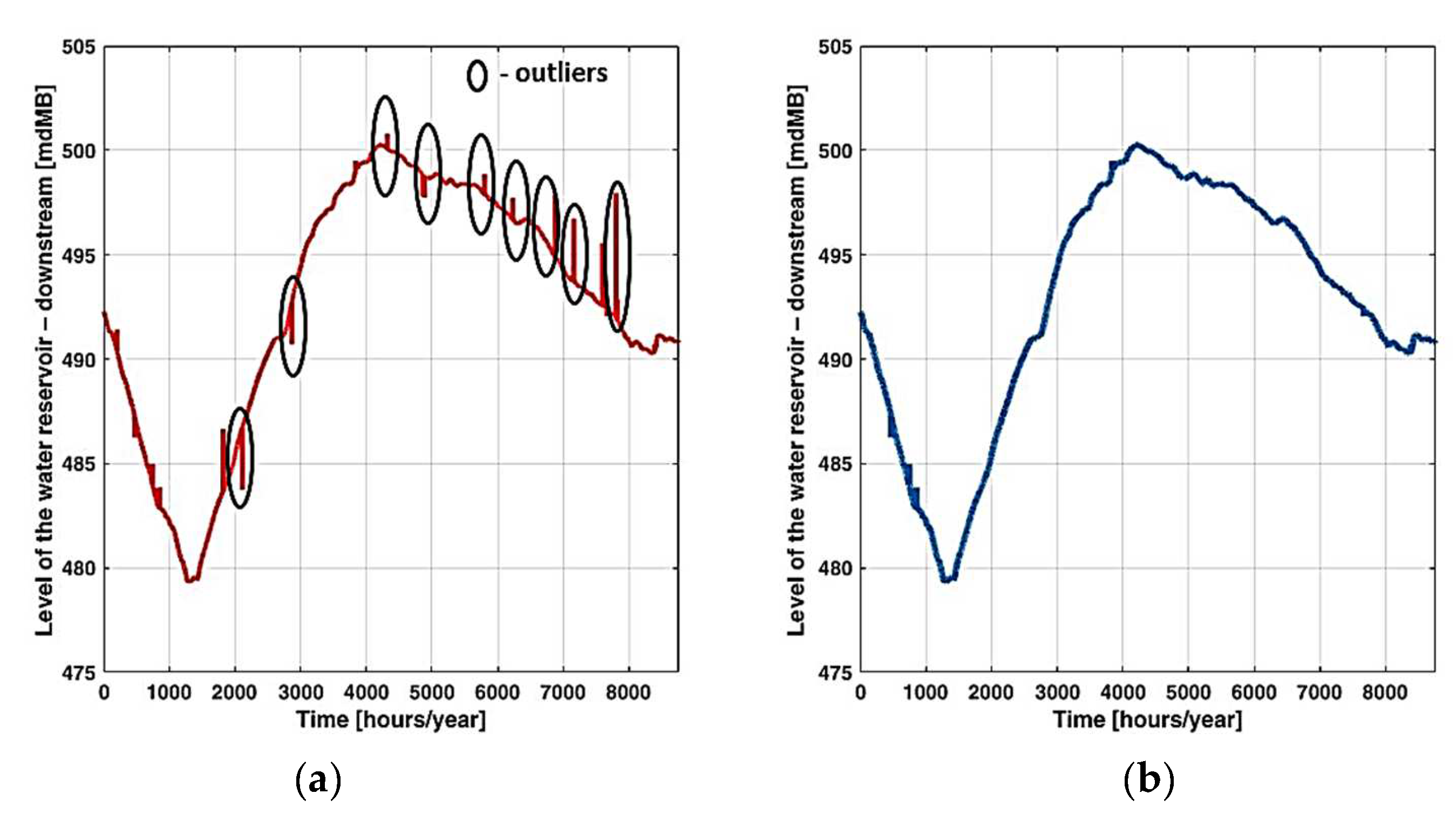
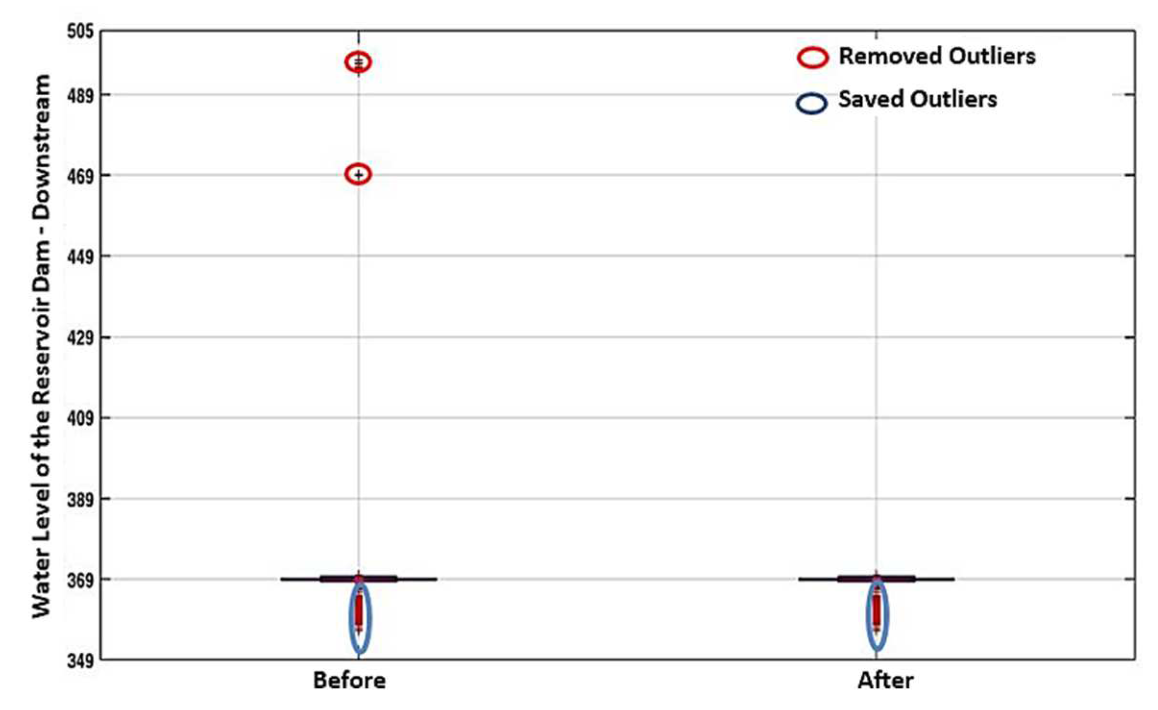
• Performing an advanced statistical analysis and outliers’ detection,
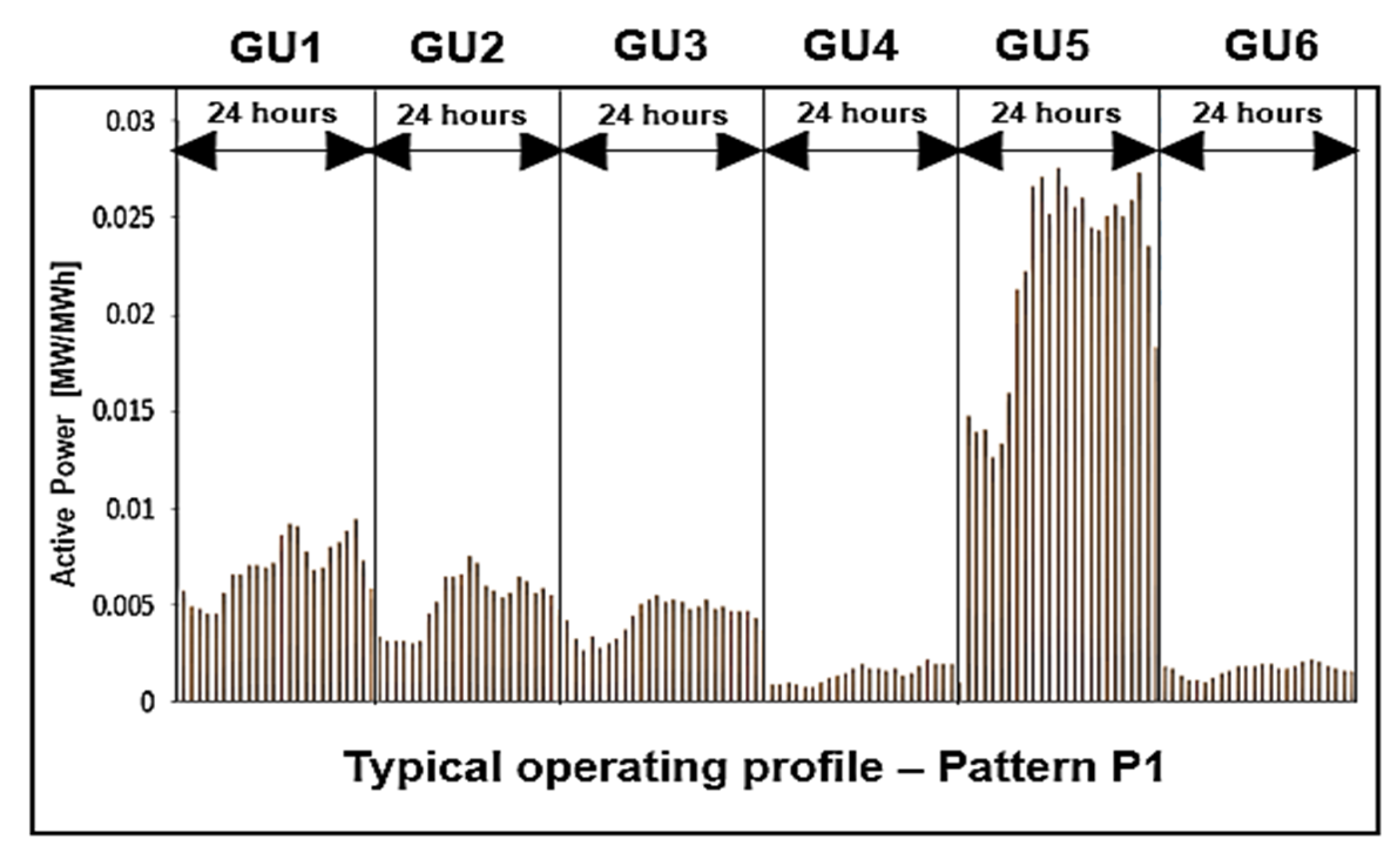
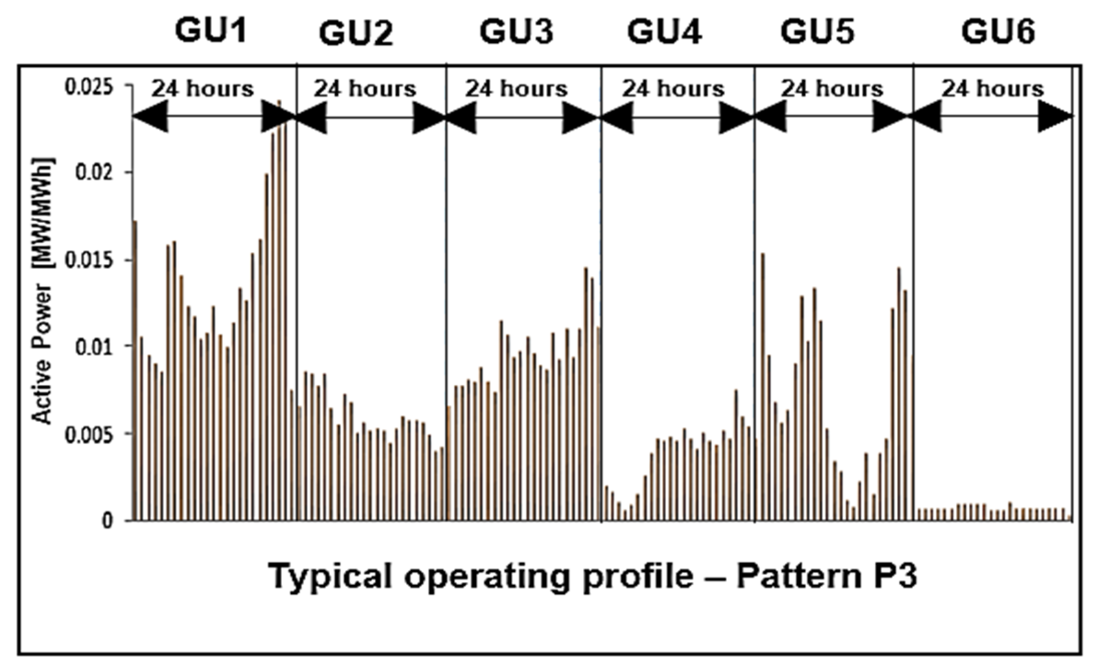
• Identifying the operating regimes and hourly typical operating profiles,
• Developing the strategies for loading the generation units that consider the number of hours of operation and the minimization of the amount of water used to satisfy the power required by the system.

The framework can offer comparative information for a time horizon longer than one year, allowing the quick identification of key performance indicators that characterize the operation of the hydropower plant.

The remainder of the paper includes four sections. Section 2 presents the theoretical aspects regarding the integration of Knowledge Discovery and Data Mining in the smart SCADA, Section 3 integrates the details on the multi-task framework integrated into the Data Mining-based Knowledge Discovery, Section 4 covers the case study where the proposed framework has been tested using the SCADA system’s database of a hydropower plant belonging to the Romanian HydroPower Company, and Section 5 highlights the conclusions and future work.

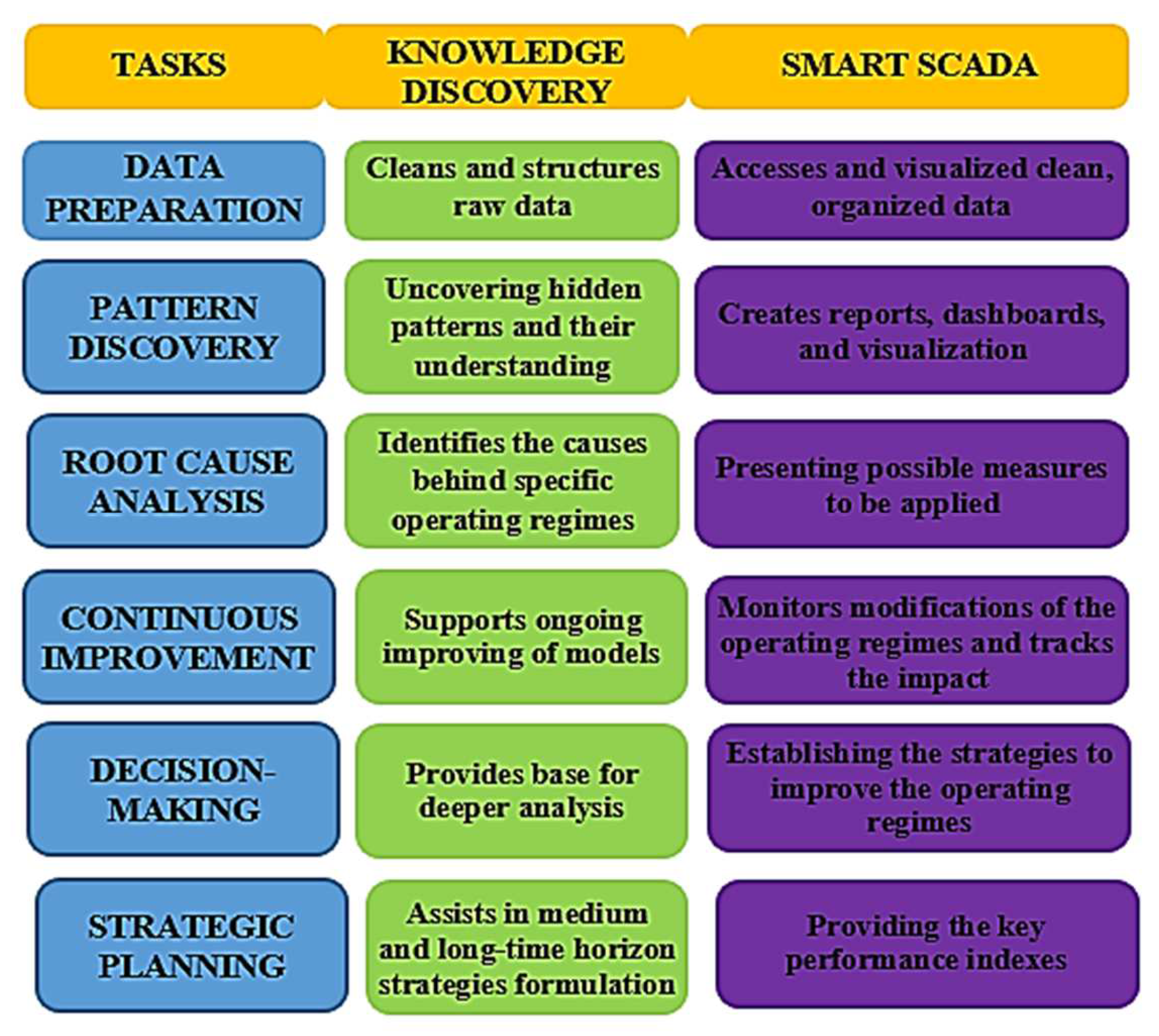
2. Knowledge Discovery and Data Mining in Smart SCADA

2.1. Knowledge Discovery vs. Data Mining

Knowledge Discovery (KD) and Data Mining (DM) have transformed the power engineering research. To carry out effective and meaningful research, a deep understanding of various aspects of data mining and knowledge discovery is necessary [23]. It includes the expertise of specialists who work in all components associated with the energy generation, transmission, and distribution of the chain representing the power system.

There are some misunderstandings about the terms data mining and knowledge discovery defined in databases. Although many specialists and researchers use DM as a synonym for knowledge discovery, DM is not the entire knowledge discovery process. In addition to being defined as data mining, it comes with other names, such as information discovery or knowledge extraction. The KD is a process that aims to identify relationships and patterns in large datasets. It is defined typically as a non-trivial process that involves identifying novel, useful, and understandable patterns. In a narrow sense, KD refers to extracting information from a data source. While it can be performed through various methods, the term refers to obtaining knowledge from textual or database data. The combined process is referred to as the KD process.

Figure 1 shows the steps of a KD process, integrating the Data Mining, and the details are introduced in the following [21,23,24].

Figure 1. The steps of a KD process.

Data Selection. KD’s initial step is data selection, which involves gathering information from the SCADA database. This process is carried out to create a raw dataset.

Data Cleaning (Preprocessing). Ensuring that the data collected are of good quality is performed through preprocessing. This process involves handling noise, missing values, and inconsistencies.

Data Transformation. After cleaning the data, it is usually necessary to transform it into something suitable for mining. This can be carried out through various methods such as feature engineering and scaling. To make it easier for the machine learning tools, the label encoding was used to convert categorical data into a more readable format.

Data Mining. The DM step involves uncovering patterns, anomalies, or relationships between the data. The DM process is composed of numerous steps, each of which is related to a specific discovery task. The extraction of knowledge involves the process of gathering and storing information. It also involves analyzing and visualizing the data, designing models for machine and human interaction, and learning how to use efficient methods. One of the most frequently used techniques is clustering, which enables us to group the data into distinct groups based on similarity.

Interpretation. After Data Mining, the next step is to interpret the results. This involves understanding the clusters (patterns) and their features.

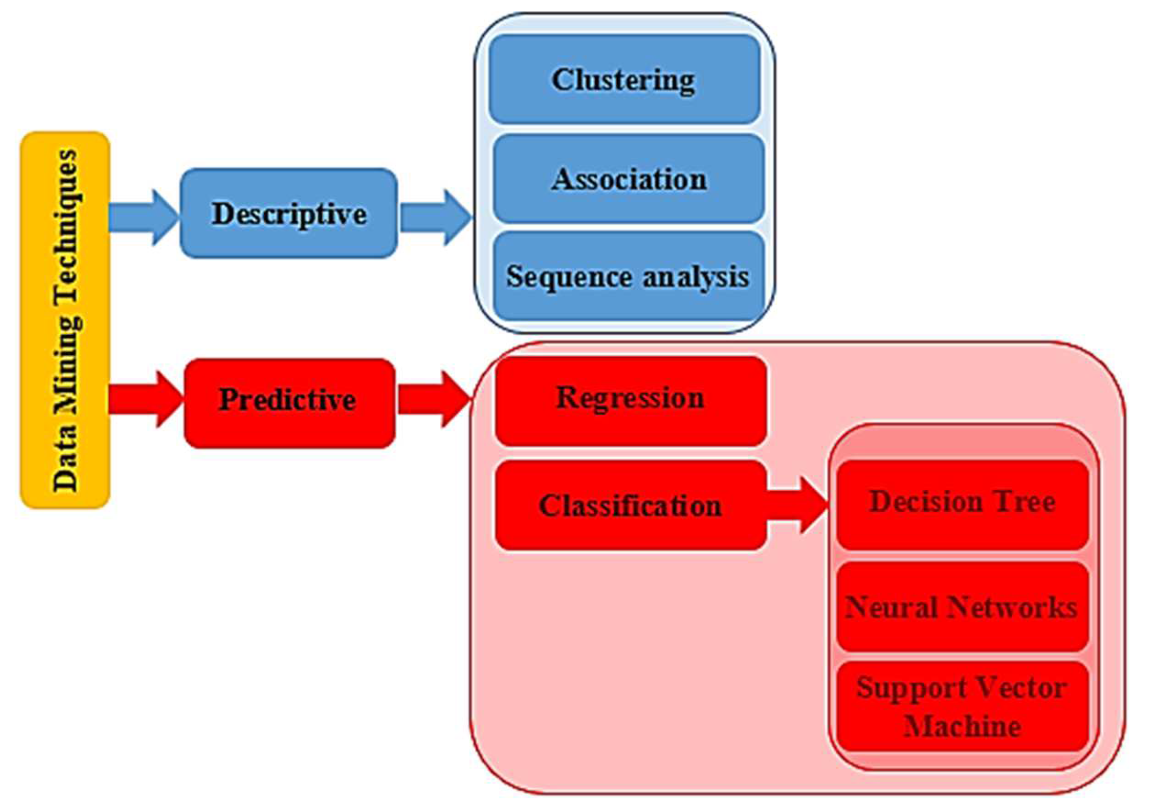
2.2. Data Mining Techniques

The Data Mining techniques are divided into two main categories: descriptive and predictive, see Figure 2 [25,26,27].

Figure 2. Data Mining techniques.

Cross-tabulation, correlation, and frequency are some of the characteristics used in the production of descriptive data mining. This process is utilized to identify the similarities between the data and the existing patterns. Another characteristic used in this type of analysis is associated with developing captivating subgroups. This is performed by analyzing the data and transforming it into meaningful information. Descriptive data mining involves techniques, such as clustering, association rule mining, and sequence discovery analysis.

Clustering. is commonly used in data mining to organize information by grouping related data points. It helps the DEMA identify patterns and similarities between different sets of information. It can be used to classify and extract patterns in the data, identify anomalies, or analyze spatial data.

Association Rules. The goal is to find the correlations in the data sets from the database. Even if the data sets come from different sources, these correlations can identify patterns that can help reveal process trends or explain the operation characteristics of the equipment/installations.

Sequence discovery analysis. The goal of sequence discovery analysis is to find interesting data sets that contain sequential patterns. This process usually involves identifying frequent patterns about a certain frequency support measure.

The second category aims to predict the future results of a given variable with a high degree of accuracy. This data mining is carried out using supervised learning techniques. There are three categories of methods that are used in this type of mining: regression, classification, and time-series analysis. The latter two are utilized in predictive analysis to model the data.

Regression. It is similar to the clustering technique in that it focuses on the relationship between a target and an independent variable. The target variables can be influenced by different predictors or independent factors, which is why a regression analysis is utilized. It predicts the outcomes based on the input fields relevant to the target.

Classification. It is carried out by identifying the various features of the data. This process helps to identify patterns and extract meaningful insights. It also helps in improving the quality of the data. The appropriate features are selected to classify it after the data has been collected and analyzed. A suitable algorithm is then chosen to implement.

• Support Vector Machine. This algorithm creates a boundary between the different classes/patterns. It identifies the features that are most important to the classification process.
• Decision Tree. The classification process is carried out using a tree-based structure. This algorithm uses a set of conditions to categorize the data. The root nodes of the structure are set for the test conditions, while the leaf nodes are for the outcome.
• Neural Network. A neural network model is a computational resource that can recognize the relationships between various data sets. These units, which act like neurons, are formed by connecting the inputs and outputs. The model considers the connection strength and outputs the information in a hidden layer. The neural network is similar to the human brain in that it requires training to be effective. Although it can be hard to interpret, the models are reliable and can even classify past training procedures.

The Smart SCADA can improve the efficiency of the hydropower plant operation by combining Knowledge Discovery and statistical analysis. Figure 3 displays the interdependencies between the Knowledge Discovery and Smart SCADA (adapted after [28]).

Figure 3. Interdependencies between the Knowledge Discovery and Smart SCADA.

Data are everything in the operation of a hydropower plant. The collection, analysis, and control actions make up the difference between classical and smart SCADA systems [29]. One of the biggest obstacles greeted by the transformation from the classic into a smart SCADA system is the lack of investment in hydropower processes. Many monitoring and control devices, representing remote terminal units and sensors from the hydropower processes, are old and should be replaced, but their upgrade is incredibly costly. The smart infrastructure integrating the data analytics modules alongside existing hardware can represent the solution for hydropower companies. If the process starts with the software part, it is much easier than replacing the hardware part. Thus, the transition from the classical to a smart SCADA system will be gradual. The goal of implementing a gradual transition is to make sure that the new system is stable before starting work on a smart SCADA infrastructure. The smart SCADA is built using knowledge discovery tools and delivers a unique and comprehensive solution for data processing from the hydropower aggregates/equipment. This holistic approach allows the fulfillment of the tasks at the hydropower plant level by the control room operator and the central level by the hydropower arrangement dispatcher.

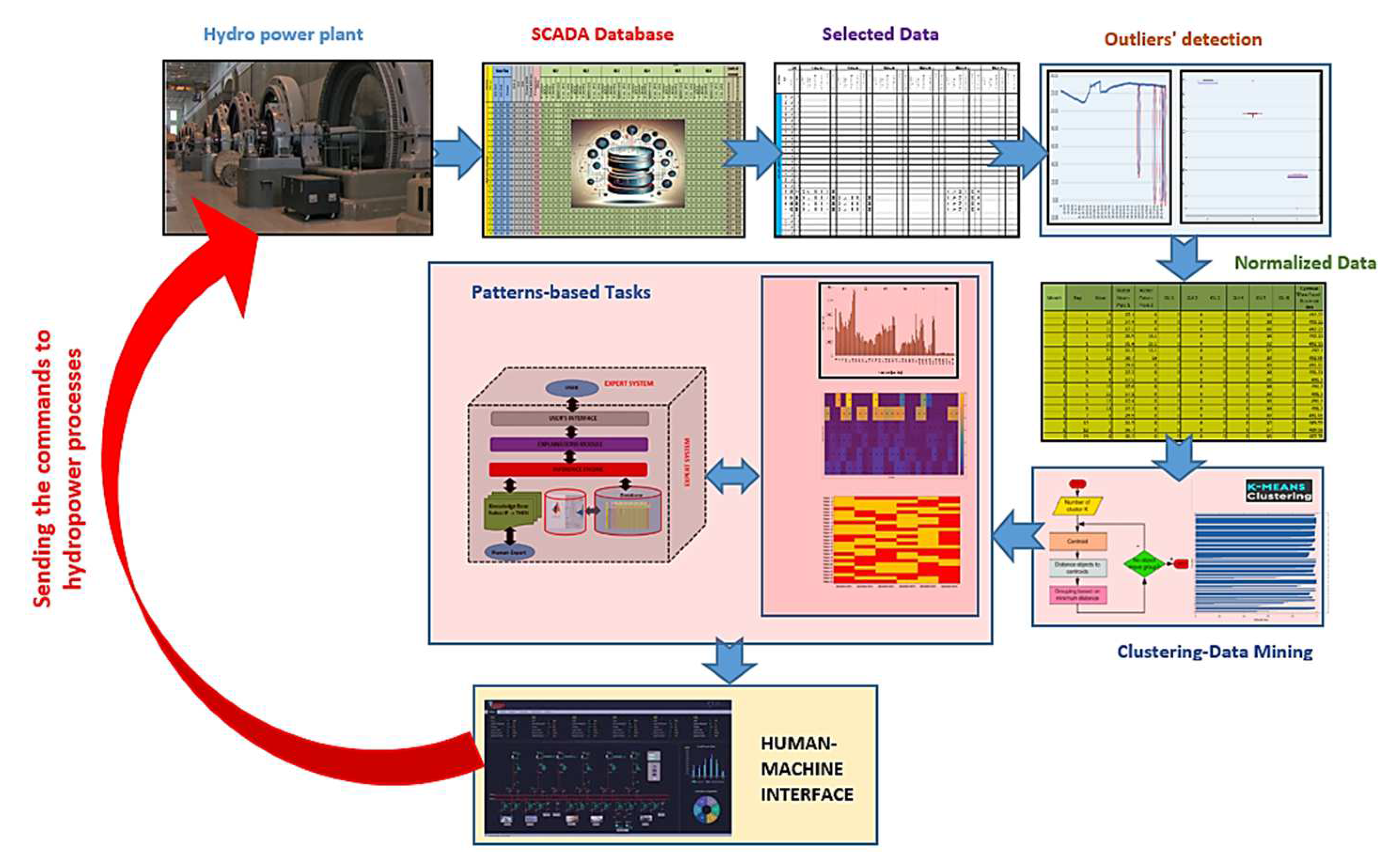
3. Multi-Task Framework Integrated into the Knowledge Discovery Module

The main steps in the multi-task framework related to developing the Knowledge Discovery module based on Data Mining to facilitate the transition from the classical to smart SCADA system in the hydropower plants are discussed in this section.

Figure 4 presents the basic structure of an automation architecture presented in [30], including the proposed Knowledge Discovery module in the SCADA system implemented at the level of the power plant.

Figure 4. The basic structure of an automation architecture including the SCADA system.

The data acquisition is performed on main hydro components (turbine, generator, power transformer, substation level), recorded in the SCADA system, and made available to the operator from the control room through the Human–Machine Interface. The Data Mining-based Knowledge Discovery module will be implemented at the SCADA level to ensure data-driven decision-making, ensuring the transition toward smart SCADA.

Figure 5 shows the flow chart of the multi-task framework integrated into the Knowledge Discovery module. Details regarding each task are provided above.

Figure 5. The multi-task framework integrated into the Knowledge Discovery module.

The SCADA system collects the water flows in the pipes that supply the turbines (WF_Pipe_1,…, WF_Pipe_n, and WF_tot_Pipes), in [m³], the active powers produced by the generation units (GUs), which are supplied through Pipe_1, …, Pipe_n (P_GU_Pipe_1, …, P_GU_Pipe_n), the requested active and reactive power of the system to the hydropower plant (P_req and Q_req), in [MW] and [MVAr]. It also contains information about the various technical parameters of the generation units, such as the active and reactive powers (P_GU1, …, P_GUn, and Q_GU1, …, Q_GUn), in [MW] and [MVAr], the stator voltage and current (Vs_GU1, …, Vs_GUn and Is_GU1, …, Is_GUn), in [kV] and [kA], the excitation voltage or current (Vex_GU1, …, Vex_GUn and Iex_GU1,…, Iex_GUn), in [V] and [A], water levels of the reservoir upstream and downstream (WLr_u and WLr_d), in [mdMB]. Appendix A includes in Table A1, as an example, the above information for a day. All variables are recorded in a table with the time details in the format month–day–hour for each year, as seen in Figure 6.

Figure 6. The fields of the SCADA database.

Task 1—Statistical analysis and outliers’ detection.

The statistical analysis is associated with exploring and presenting large amounts of data on the technical parameters based on the parameters such as mean, standard deviation, confidence degree, and quintiles-Q0 (minimum value), Q1 (25th), Q2 (50th), Q3 (75th), and Q4 (maximum value). Also, the boxplot is used to show the spread and skewness of the variables from the database through their quintiles. It can also include lines known as whiskers, which extend from the box to indicate variability outside the lower and upper limits of the dataset. Outliers with significant differences from the rest of the data can be plotted on the box-and-whisker diagram [31]. Thus, the DEMA (represented by the operator from the control room) can select the fields containing the values of the monitoring parameters. Regarding the outliers’ detection, a rules-based algorithm based on the values of the quintiles has been integrated [32,33]. These two rules refer to Q0 and Q4:

If < X^h < Q0^x > then < X^h is outlier >

(1)

If < X^h > Q4^x > then < X^h is outlier>

(2)

where X^h is the hourly value of the analyzed technical parameter and x refers to the name of the analyzed technical parameter (identically with the name of the field).

However, there are cases when the outliers identified for certain technical parameters can be associated with the different operating regimes compared to most regimes but which do not lead to the violation of the allowable limits. In these cases, an attention message will alert the DEMA, who will verify only those regimes. For all other cases, when the outliers are identified, the least squares method is applied to estimate the “true” value. The approach is based on a regression model determined for that parameter.

A comparison between more years can be performed by choosing the analysis period.

Task 2—Determining the operating regimes.

This task is based on the clustering-based data mining process. The input data are associated with a matrix structure built with the values of technical parameters selected by the DEMA. The regimes are identified through the typical operating profiles divided into the intervals associated with the generating units (GU1, …, GUn) or hourly loading patterns, including the hourly average power of each generation unit. The DEMA can choose any algorithm from the hierarchical clustering category (complete-linkage clustering, single-linkage clustering, average linkage clustering, centroid linkage clustering, median linkage clustering, or Ward linkage clustering) or K-means clustering algorithm. In hierarchical clustering, a similarity measure between the sets of observations is necessary to determine which patterns should be grouped or separated. Usually, in hierarchical clustering, the set’s similarity is determined by using a distance between the observations. It is carried out through a linkage criterion that specifies the set’s similarity.

When the DEMA requests characterization of the operating regimes through the typical operating profiles, then the matrix structure of the input data corresponding to the clustering process is identified with the fields of the active power produced by each generation unit in a certain time horizon (usually a year to cover all operating regimes).

The matrix size is H_year × (N_HPP^GU × 24 + 2), where H_year represents the number of hours when at least one generation unit worked and N_HPP^GU represents the number of the generation units from the hydropower plant. The additional columns correspond to the water levels of the reservoir—upstream and downstream.

Each obtained pattern is associated with a typical operating profile that characterizes the operating regime of the hydropower plant in certain periods (days inside a year). The DEMA can identify the operating regimes of the hydropower plant through an evolution along the time axis of the degree of hourly loading of all generating units and the water volume used in each operating regime. The DEMA can establish an operating strategy for the plant for the next day depending on the forecasting of the requested powers by the system.

The input data matrix is different when the DEMA’s requests are as the operating regimes to be characterized through hourly loading patterns. The structure is identified with the fields of the active power produced by each generation unit in a certain time horizon (usually a year to cover all operating regimes). The size of the matrix is H_year × (N_HPP^GU + 2), where H_year and N_HPP^GU have the same signification as above. The last two columns correspond to the water levels of the reservoir.

Task 3—Developing the strategies to load the generation units.

The task is associated with an expert system that uses the operating regimes to be characterized by hourly loading patterns determined above and the number of hours of operation. This last information is recorded in a database and considered in the decision-making process to avoid overloading the generation units over a long period, which leads to minimizing the number of maintenance operations. Using a water amount to satisfy the power required by the system represents the main objective. The main components of the expert system are presented synthetically in the following [34,35].

• The knowledge base is composed of two main elements: the rules base (which contains the knowledge required to solve problems) and the facts base (the patterns obtained in the clustering-based data mining are recorded in this base).
• The inference engine can determine the mode in which knowledge derived from the rules base is utilized to interpret the data from the information base. It can perform various tasks, such as confirming or rejecting a hypothesis or the solution of a problem.
• The editor of the knowledge base provides the DEMA with the ability to update and inspect the information base’s content, particularly its rules base’s content.
• The explanation system can provide explanations for the stages in the Expert System’s reasoning.

4. Case Study

The proposed framework has been tested using the SCADA system’s database of a hydropower plant belonging to the Romanian HydroPower Company.

The plant, identified through the red circle in Figure 7, is the first from a hydro arrangement located on an important river in eastern Romania. The plant has six Francis-type units. The first water pipe supplies the last two units, and the second piper the first four units. The first four units have a total installed power of 27.5 MW, while units five and six have 50 MW.

Figure 7. The hydro arrangement of which the analyzed plant is a part (adapted after [36,37]).

The SCADA database includes fields completed at every hour with the following technical parameters: the individual water flows of each pipe, the total water flow of the two pipes, the total produced power of the first four-generation units (GU1–GU4), the produced power by the GU5, the produced power by the GU6, the total produced active and reactive power by the plant, the frequency, the stator voltage, the stator current, the produced active and reactive powers, the excitation voltage, the excitation current of each generation unit, and water levels of the reservoir (upstream and downstream).

The SCADA file associated with a day from the database containing the fields highlighted above is shown in Figure 8. The signification of the blank cells corresponds with the case of the non-loading of the generation unit. The obtained results at the year level for each task integrated into the proposed framework are presented in the following.

Figure 8. SCADA file associated with a day from the database.

The DEMA can see after data processing the summary information on the operation of the plant regarding the number of hours and the total energy produced by each generation unit (GU1–GU2), see Figure 9.

Figure 9. The summary information regarding the operation of the plant regarding the number of hours and the total energy produced by each generation unit.

Table 1 presents the extracted results from the advanced statistical analysis containing the mean (m), standard deviation (σ), and quintiles (Q0, Q1, Q2, Q3, and Q4) for each technical parameter from the database. The values have been calculated only for the hours when at least one unit was in operation. Also, the DEMA has available boxplots from which outliers are identified quickly.

Table 1. The extracted results from the statistical analysis.

Statistical Parameters		m	σ	Q0	Q1	Q2	Q3	Q4
Water flow	WF_Pipe1 [m3/s]	36.42	9.75	18.70	31.50	34.50	36.30	74.40
	WF_Pipe2 [m3/s]	29.92	14.02	13.40	17.30	30.80	36.60	78.20
	Total [m3/s]	56.14	21.35	10.50	44.50	54.10	70.80	133.20
Active and reactive powers	GU1-GU4 [MW]	29.60	13.54	0.90	18.00	30.00	37.00	78.00
	GU5 [MW]	34.33	3.09	29.00	31.00	35.00	37.00	40.00
	GU6 [MW]	31.51	2.01	1.00	30.00	31.00	33.00	40.00
	Total [MW]	56.34	20.39	13.00	45.00	56.00	72.00	126.00
	Total [MVAr]	6.39	5.90	1.00	2.00	3.00	10.00	30.00
Frequency	[Hz]	49.99	0.02	49.10	49.98	50.00	50.01	50.40
GU 1	Vs [kV]	10.43	0.71	1.40	10.40	10.40	10.50	50.00
	Is [kA]	0.96	0.11	0.08	0.90	0.95	1.00	1.90
	P [MW]	17.20	1.89	0.90	15.00	17.00	18.00	22.00
	Q [Mvar]	2.60	1.99	1.00	1.00	1.00	5.00	11.00
	Vex [V]	88.28	8.80	8.00	80.00	90.00	95.00	110.00
	I ex [A]	287.91	17.29	100.00	280.00	290.00	300.00	360.00
GU 2	Vs [kV]	10.48	0.38	1.10	10.50	10.50	10.50	10.70
	Is [kA]	0.96	0.10	0.70	0.90	0.95	1.05	1.20
	P [MW]	17.35	1.86	14.00	16.00	17.00	19.00	21.00
	Q [Mvar]	2.58	1.99	1.00	1.00	1.00	5.00	21.00
	Vex [V]	89.84	7.80	70.00	85.00	90.00	95.00	110.00
	I ex [A]	289.65	15.01	245.00	280.00	290.00	300.00	320.00
GU 3	Vs [kV]	10.41	0.42	1.60	10.40	10.50	10.50	10.70
	Is [kA]	0.91	0.08	0.70	0.85	0.90	0.95	1.15
	P [MW]	16.48	1.41	13.00	15.00	16.00	17.00	20.00
	Q [Mvar]	2.76	2.00	0.50	1.00	1.00	5.00	10.00
	Vex [V]	89.60	40.80	65.00	80.00	90.00	95.00	870.00
	I ex [A]	289.21	58.37	115.00	280.00	290.00	300.00	2980.00
GU 4	Vs [kV]	10.45	0.09	10.10	10.40	10.50	10.50	10.60
	Is [kA]	0.92	0.08	0.75	0.85	0.90	1.00	1.10
	P [MW]	16.59	1.36	14.00	15.00	17.00	18.00	20.00
	Q [Mvar]	2.78	1.99	1.00	1.00	1.00	5.00	5.00
	Vex [V]	87.38	8.87	60.00	80.00	90.00	95.00	105.00
	I ex [A]	290.13	15.75	260.00	280.00	290.00	300.00	330.00
GU 5	Vs [kV]	10.41	0.52	1.40	10.40	10.50	10.50	10.70
	Is [kA]	1.89	0.17	0.85	1.70	1.90	2.05	2.70
	P [MW]	34.33	3.09	29.00	31.00	35.00	37.00	40.00
	Q [Mvar]	2.56	1.96	1.00	1.00	1.00	5.00	10.00
	Vex [V]	104.78	17.89	10.00	100.00	100.00	110.00	1110.00
	Iex [A]	332.53	108.88	235.00	315.00	330.00	340.00	3210.00
GU 6	Vs [kV]	10.49	0.07	10.30	10.50	10.50	10.50	10.60
	Is [kA]	1.70	0.07	1.50	1.65	1.70	1.75	1.85
	P [MW]	31.52	1.33	29.00	30.00	31.00	33.00	33.00
	Q [Mvar]	2.07	1.77	1.00	1.00	1.00	5.00	5.00
	Vex [V]	94.47	6.15	80.00	90.00	95.00	100.00	110.00
	I ex [A]	303.34	10.77	280.00	300.00	300.00	310.00	340.00
Water level	WLr_u [mdMB]	492.66	5.86	479.28	489.80	493.40	497.99	500.80
	WLr_d [mdMB]	368.21	5.90	356.43	368.90	369.06	369.20	497.48

Two situations are presented in the following. The first refers to the loading of the generation units when the outliers identified associated with the different operating regimes compared to most regimes did not lead to the violation of the allowable limits, see Figure 10. In these cases, an attention message is launched to the DEMA, who must verify the regimes and establish if any disturbance appeared.

Figure 10. The boxplots corresponding to the loading of the generation units over a period of one year.

The second situation belongs to the downstream level of the water reservoir recorded, where more outliers have been identified exceeding the upper limit. For these values, the least squares method has been applied to estimate the “true” value.

In the case of the outliers below Q0, these depend on the upstream level of the water reservoir, which did not lead to the violation of the allowable limits. Figure 11 and Figure 12 present the results obtained in these cases (with and without outliers over the maximum limit).

Figure 11. The values corresponding to the level of the water reservoir—downstream ((a) taken from the database containing outliers; (b) after data processing, without outliers).

Figure 12. The boxplots corresponding to the level of the water reservoir—downstream.

The second task refers to determining the operating regimes identified through the typical operating profiles divided into the intervals associated with the generating units (GU1, …, GU6) and hourly loading patterns, including the hourly average power of each generation unit. This task is based on the clustering-based data mining process.

The input data have been associated with a matrix structure built with the values of hourly active powers of all six generation units selected from the database from three successive years (2017–2019). The K-means clustering algorithm has been used to obtain the typical operating profiles presented in Figure 13, Figure 14, Figure 15 and Figure 16.

Figure 13. The typical operating profile of the hydropower plant assigned to pattern P1.

Figure 14. The typical operating profile of the hydropower plant assigned to pattern P2.

Figure 15. The typical operating profile of the hydropower plant assigned to pattern P3.

Figure 16. The typical operating profile of the hydropower plant assigned to pattern P4.

Appendix A includes in Table A2, Table A3, Table A4 and Table A5 the hourly values of each operating regime (identified through the Patterns P1–P4) containing the typical operating profiles divided into the intervals associated with the generating units (GU1, …, GU6). The input data used to obtain hourly loading patterns contain the following fields: water flows on the two pipes, the loading of each generator unit, and the upstream and downstream water level of the reservoir.

The K-means clustering algorithm has been used to extract the patterns, and the optimal number has been 25. Figure 17, Figure 18 and Figure 19 show how the hydropower plant has been operated based on the obtained patterns of hourly loading of the generation units in three consecutive years, 2017–2019.

Figure 17. The patterns obtained for the hourly loading of the generation units in 2017.

Figure 18. The patterns obtained for the hourly loading of the generation units in 2018.

Figure 19. The patterns obtained for the hourly loading of the generation units in 2019.

Annex A includes in Table A6 and Table A7 details of the patterns regarding the hourly loading of the generation units and their features regarding the operating conditions in an analyzed three-year period. This task improves the quality of the obtained solutions and the decision-making processes that are involved in the loading of the generation units.

The third task is based on an expert system involved inside the module that analyzes the hourly patterns and operating conditions of the units to determine the optimal loading solution depending on the number of operating hours and the power requested by the system. Figure 20, Figure 21 and Figure 22 present the obtained results for a representative day from 2020.

Figure 20. The active power requested by the system.

Figure 21. The active power distributed among the six GUs—the strategy adopted by the DM without the Knowledge Discovery module.

Figure 22. The active power distributed among the six GUs—the strategy adopted by the DM based on the Knowledge Discovery module.

It can be observed that the loading of the six GUs is different in the developed strategy compared with the experience-based strategy adopted by DEMA. Table 2 presents the differences between the experience-based strategy and the expert system-based developed strategy. The signification of the colors is the following:

Table 2. The differences between the experience-based strategy and expert system-based strategy.

Hour	P_GU1 [MW]	P_GU2 [MW]	P_GU3 [MW]	P_GU4 [MW]	P_GU5 [MW]	P_GU6 [MW]
1	+16	0	−16	0	0	0
2	+16	0	−16	0	0	0
3	+16	0	−16	0	0	0
4	+16	0	−16	0	0	0
5	+16	0	−16	0	0	0
6	+16	0	−16	0	0	0
7	+16	0	−16	0	0	0
8	−1	+17	+1	+17	−34	0
9	−1	+17	+1	+17	−34	0
10	−1	+17	+1	+17	−34	0
11	−1	0	−1	0	−34	+36
12	−1	0	−1	0	−34	+36
13	+16	0	−16	0	0	0
14	+16	0	−16	0	0	0
15	+16	0	−16	0	0	0
16	16	0	−16	0	0	0
17	0	0	+2	0	+38	−40
18	0	0	+2	0	+38	−40
19	+16	0	−16	0	0	0
20	+15	+16	0	+15	0	−46
21	+15	+16	0	+15	0	−46
22	+15	+16	0	+15	0	−46
23	+15	+16	0	+15	0	−46
24	+15	+16	0	+15	0	−46

• Red color is associated with the generation units that have been loaded in the experience-based strategy but not considered in the case of the expert system-based strategy (the sign is “-“).
• Blue color is associated with the generation units that have been loaded in the expert-based strategy but not considered in the case of the experience-based strategy (only with the sign “+“).
• Green color is associated with the generation units loaded in the expert-based strategy, having the same (value “0”) or having another loading in the expert-based strategy (with signs “+“ or “−“).
• Yellow color is associated with the generation units that have not been loaded in either strategy.

The proposed strategy adopted a loading of the first four GUs between 60 and 72% of the rated power with the loading of GU5 and GU6 only for powers required by the system with higher values. These generation units will be available for ancillary services.

Table 3 presents the specific indicators for each GU obtained for operating the HPP in 2020 with the proposed strategy regarding the total operating time, the total energy production, and the average loading.

Table 3. The specific indicators for each GU obtained for operating the HPP in 2020.

Generation Unit	GU1	GU2	GU3	GU4	GU5	GU6	HPP
Operating time [hours]	3460	1970	1520	1484	1271	3255	12960
Energy production [TWh]	72.33	40.60	29.3	28.26	46.37	161.85	378.71
Average loading [MW]	21	21	19	19	36	50	166

A comparison between results obtained with the adopted expert system-based strategy in 2020 and those obtained with the experience-based strategy in 2017 revealed an increase in the average loading for all six GUs with 21.5% (GU1), 18.9% (GU2), 16.9% (GU3), 14.8% (GU4), 6.3% (GU5), and 57.7% (GU6). The smallest increase has been observed in the case of GU5, the most elevated has been obtained for GU6, and between 14.8% and 21.5% for the first four GUs. However, the higher loading of UG6 was because it was in maintenance operation for two years and worked for very few hours during that time. The total energy production has increased by 20.8% from 313.6 TWh to 378.7 TWh, although the total operating time of all GUs decreased by 5.1% from 13,653 h to 12,960 h. The years 2018 and 2019 are not considered in our analysis because GU6 stopped in 2018 and had a few hours of operation in 2019.

5. Conclusions

As the world moves toward a more sustainable energy future, the need for more reliable and dispatchable sources of electricity is increasing. An important factor that can help improve the optimal operation of hydropower plants is associated with quick data processing and extracting hidden patterns. Knowledge discovery can represent an efficient tool for addressing various challenges, among which is the optimal operation of hydropower plants.

This paper proposes a framework that combines data mining and knowledge discovery to help the transition from a traditional SCADA system to a smart one in hydropower plants. It will allow the DEMA (operators from the control room) to identify the outliers and implement effective strategies to minimize water consumption and maximize power generation. Based on the advanced statistical tools, the framework will also help them identify the optimal operating conditions for the plant. The performance has been tested in a Romanian hydropower plant using the SCADA database. It allowed the control room operators to obtain comparative information on the plant’s performance over a longer time horizon (in our case study, three years). The results of the tests revealed the utility of a knowledge discovery module in helping the control room operators improve the efficiency of their operations by transitioning toward smart SCADA systems. Thus, a comparison between results obtained with the adopted expert system-based strategy in 2020 and those obtained with the experience-based strategy in 2017 revealed an increase in the average loading at the level of the HPP from 133 MW to 166 MW (representing the sum of powers produced by all six GUs), which means that the HPP was loaded from 64% to 80% of the total installed power of 210 MW. Also, the total energy production has increased by 20.8%, although the total operating time of all GUs decreased by 5.1%.

The future of work is characterized by developing a new task associated with the uncertainty modeling of two variables: the hourly powers requested by the system and the upstream level in the water reservoir. The modeling of the first variable is based on the results obtained with a forecasting method, having the input data rainfall, temperature, and historical values recorded in the SCADA database. The operating regime of the hydro cascade, of which the plant is a part, and the historical data from the other plants represent the factors used in the developed models for the second variable. This new task will be a new component of the Data Mining-based Knowledge Discovery Module to determine quickly the best strategy to load the generation units in uncertain conditions.

References

- International Hydropower Association. World Hydropower Outlook. Opportunities to Advance Net Zero. 2024. Available online: https://www.hydropower.org/publications/2024-world-hydropower-outlook (accessed on 5 September 2024).
- Parvez, I.; Shen, J.; Hassan, I.; Zhang, N. Generation of Hydro Energy by Using Data Mining Algorithm for Cascaded Hy-dropower Plant. Energies 2021, 14, 298. [Google Scholar] [CrossRef]
- International Energy Agency. Hydropower Special Market Report Analysis and Forecast to 2030. 2021. Available online: https://iea.blob.core.windows.net/assets/83ff8935-62dd-4150-80a8-c5001b740e21/HydropowerSpecialMarketReport.pdf (accessed on 5 September 2024).
- Essenfelder, A.H.; Larosa, F.; Broccoli, D.; Mazzoli, P.; Bagli, S.; Luzzi, V.; Mysiak, J.; dalla Vallw, F. Smart Climate Hydro-power Tool: A Machine-Learning Seasonal Forecasting Climate Service to Support Cost–Benefit Analysis of Reservoir Management. Atmosphere 2020, 11, 1305. [Google Scholar] [CrossRef]
- Garbea, R.; Scarlatache, F.; Grigoras, G.; Neagu, B.C. Extracting the Operating Characteristics of Hydropower Plants Using a Clustering-based Efficient Methodology. In Proceedings of the IEEE 9th International Conference on Modern Power Systems (MPS), Cluj-Napoca, Romania, 16–17 June 2021. [Google Scholar]
- International Finance Corporation. Hydroelectric Power. A Guide for Developers and Investors. 2024. Available online: https://documents1.worldbank.org/curated/en/917841468188335073/pdf/99392-WP-Box393199B-PUBLIC-Hydropower-Report.pdf (accessed on 5 September 2024).
- International Renewable Energy Agency. Renewable Energy Technologies: Cost Analysis Series. Hydropower. 2012. Available online: https://www.irena.org/-/media/Files/IRENA/Agency/Publication/2012/RE_Technologies_Cost_Analysis-HYDROPOWER.pdf (accessed on 5 September 2024).
- Eker, O.F. Data Science for Industry: Hydropower Condition Monitoring and Predictive Maintenance. 2022. Available online: https://medium.com/@omerfarukeker/data-science-for-industry-hydropower-condition-monitoring-and-predictive-maintenance-49952215fdd7 (accessed on 31 July 2024).
- Quaranta, E.; Aggidis, G.; Boes, R.; Comoglio, C.; De Michele, C.; Ritesh Patro, E.; Georgievskaia, E.; Harby, A.; Kougias, I.; Muntean, S.; et al. Assessing the energy potential of modernizing the European hydropower fleet. Energy Convers. Manag. 2021, 246, 114655. [Google Scholar] [CrossRef]
- Betti, A.; Crisostomi, E.; Paolinelli, G.; Piazzi, A.; Ruffini, F.; Tucci, F. Condition Monitoring and Predictive Maintenance Methodologies for Hydropower Plants Equipment. Renew. Energy 2021, 171, 246–253. [Google Scholar] [CrossRef]
- European Commission. 2050 Long-Term Strategy. Striving to Become the World’s First Climate-Neutral Continent by 2050. Available online: https://climate.ec.europa.eu/eu-action/climate-strategies-targets/2050-long-term-strategy_en (accessed on 5 September 2024).
- Ovarro. Five Ways SCADA Systems Can Benefit Sustainability: Although Hidden in the Background, SCADA Systems Are Crucial to Energy Savings. 2024. Available online: https://www.linkedin.com/pulse/five-ways-scada-systems-can-benefit-sustainability-although-hidden-sbdae/ (accessed on 31 July 2024).
- Yang, S.; Stempfle, T.; Thiede, S.; Lanza, G. Approach for the Development of a Sustainability-oriented Implementation Strategy of Smart Automation Technologies. Procedia CIRP 2024, 122, 849–854. [Google Scholar] [CrossRef]
- Vagnoni, E.; Gezer, D.; Anagnostopoulos, I.; Cavazzini, G.; Doujak, E.; Hočevar, M.; Rudolf, P. The New Role of Sustainable Hydropower in Flexible Energy Systems and its Technical Evolution Through Innovation And Digitalization. Renew. Energy 2024, 230, 120832. [Google Scholar] [CrossRef]
- Feng, Z.K.; Niu, W.J.; Zhang, R.; Wang, S.; Cheng, C.-T. Operation Rule Derivation of Hydropower Reservoir by K-Means Clustering Method and Extreme Learning Machine Based on Particle Swarm Optimization. J. Hydrol. 2019, 576, 229–238. [Google Scholar] [CrossRef]
- Zhang, F.; Guo, J.; Yuan, F.; Qiu, Y.; Wang, P.; Cheng, F.; Gu, Y. Enhancement Methods of Hydropower Unit Monitoring Data Quality Based on the Hierarchical Density-Based Spatial Clustering of Applications with a Noise–Wasserstein Slim Generative Adversarial Imputation Network with a Gradient Penalty. Sensors 2024, 24, 118. [Google Scholar] [CrossRef] [PubMed]
- Luo, W.; Xu, J.; Zhou, Z. Mobile Information Systems, Retracted: Design of Data Classification and Classification Management System for Big Data of Hydropower Enterprises Based on Data Standards, Mobile Information Systems. 2022. Available online: https://onlinelibrary.wiley.com/doi/10.1155/2022/8103897 (accessed on 31 July 2024).
- Ahmed, I.; Dagnino, A.; Bongiovi, A.; Ding, Y. Outlier Detection for Hydropower Generation Plant. In Proceedings of the IEEE 14th International Conference on Automation Science and Engineering (CASE), Munich, Germany, 20–24 August 2018. [Google Scholar]
- Valencia, A.M.; Caratar, J.; Caicedo, G.; Chamorro, C. Proposal for a KDD-Based Procedure to Obtain a Set of Intelligent Systems Training Applied to the Identification of Failures in Hydroelectric Power Plants. J. Appl. Res. Technol. 2021, 18, 376–389. [Google Scholar] [CrossRef]
- Zhang, W.; Ge, Y.; Liu, G.; Qi, W.; Xu, S.; Peng, Z.; Li, Y. Clustering and Decision Tree Based Analysis of Typical Operation Modes of Power Systems. Energy Rep. 2023, 9, 60–69. [Google Scholar] [CrossRef]
- Garbea, R.; Scarlatache, F.; Grigoras, G.; Neagu, B.C. Integration of Data Mining Techniques in SCADA System for Optimal Operation of Hydropower Plants. In Proceedings of the IEEE 13th International Conference on Electronics, Computers and Artificial Intelligence (ECAI), Pitesti, Romania, 1–3 July 2021. [Google Scholar]
- Sahin, M.E.; Ozbay Karakus, M. Smart Hydropower Management: Utilizing Machine Learning and Deep Learning Method to Enhance Dam’s Energy Generation Efficiency. Neural Comput. Appl. 2024, 36, 11195–11211. [Google Scholar] [CrossRef]
- Shu, X.; Ye, Y. Knowledge Discovery: Methods from Data Mining and Machine Learning. Soc. Sci. Res. 2023, 110, 102817. [Google Scholar] [CrossRef] [PubMed]
- Monika; Shauib, M. Implementation Platforms and Strategy for the Knowledge Discovery from the Data. In Proceedings of the International Conference on Computational Modelling, Simulation and Optimization (ICCMSO), Pathum Thani, Thailand, 23–25 December 2022. [Google Scholar]
- Ghongade, T.G.; Khobragade, R.N. Evaluation on Utilization and Emaciation of Data Mining Techniques in Information System. In Proceedings of the OPJU International Technology Conference on Emerging Technologies for Sustainable Development (OTCON), Raigarh, Chhattisgarh, India, 8–10 February 2023. [Google Scholar]
- Järvinen, P.; Siltanen, P.; Kirschenbaum, A. Data Analytics and Machine Learning. In Big Data in Bioeconomy; Södergård, C., Mildorf, T., Habyarimana, E., Berre, A.J., Fernandes, J.A., Zinke-Wehlmann, C., Eds.; Springer Nature: Cham, Switzerland, 2021; pp. 129–146. [Google Scholar]
- Garbea, R.; Grigoras, G. Clustering-Using Data Mining-based Application to Identify the Hourly Loading Patterns of the Generation Units from the Hydropower Plants. In Proceedings of the IEEE International Conference and Exposition on Electrical and Power Engineering (EPE), Iasi, Romania, 20–22 October 2022. [Google Scholar]
- Odrynska, A. What is Data Mining: Definition, Process, Techniques and Role in Business Intelligence. 2023. Available online: https://www.alphaservesp.com/blog/what-is-data-mining-definition-process-techniques-and-business-intelligence (accessed on 31 July 2024).
- Onlogic. Setting Up Smart SCADA for Digital Transformation. 2024. Available online: https://www.onlogic.com/blog/smart-scada-digital-transformation (accessed on 5 September 2024).
- Kaur, S.; Kathpal, N.; Munjal, N. Role of SCADA in Hydro Power Plant Automation. Int. J. Adv. Res. Electr. Electron. Instrum. Eng. 2015, 4, 8085–8090. [Google Scholar]
- Mirzargar, M.; Whitaker, R.T.; Kirby, R.M. Curve Boxplot: Generalization of Boxplot for Ensembles of Curves. IEEE Trans. Vis. Comput. Gr. 2023, 20, 2654–2663. [Google Scholar] [CrossRef] [PubMed]
- Chelaru, E.; Grigoras, G. Decision Support System to Determine the Replacement Ranking of the Aged Transformers in Electric Distribution Networks. In Proceedings of the IEEE 12th International Conference on Electronics, Computers and Artificial Intelligence (ECAI) Proceedings, Bucharest, Romania, 25–27 June 2020. [Google Scholar]
- Neagu, B.C.; Grigoras, G.; Scarlatache, F. Outliers Discovery from Smart Meters Data Using a Statistical Based Data Mining Approach, In Proceedings of the IEEE 10th International Symposium on Advanced Topics in Electrical Engineering (ATEE), Bucharest, Romania, 23–25 April 2017.
- Wang, Z.; Wang, S.; Zhang, S.; Zhan, J. An Expert System Based on Data Mining for a Trend Diagnosis of Process Parameters. Processes 2023, 11, 3311. [Google Scholar] [CrossRef]
- Dandea, V.; Grigoras, G. Expert System Integrating Rule-Based Reasoning to Voltage Control in Photovoltaic-Systems-Rich Low Voltage Electric Distribution Networks: A Review and Results of a Case Study. Appl. Sci. 2023, 13, 6158. [Google Scholar] [CrossRef]
- Dunca, G.; Ghergu, C.M.; Rosioru, O.; Bucur, M.D. Analysis of the Areas with Optimal Working of Aggregates in CHE Stejaru, Symposium on Informatics, Automation and Telecommunications in Energy, Sinaia, Romania. 2010. Available online: https://www.researchgate.net/publication/281646497_Analiza_zonelor_cu_functionare_optima_ale_agregatelor_din_CHE_Stejaru (accessed on 31 July 2024). (In Romanian).
- Cojoc, G.M. Analysis of The Hydrological Regime of the Bistrita River in the Context of Hydrotechnical Developments; Terra Nostra Publishing House: Iasi, Romania, 2016. [Google Scholar]