Complex Network Modeling and Analysis of Microfracture Activity in Rock Mechanics

Abstract

This study employs rock triaxial acoustic emission laboratory tests to investigate the activity of microfractures in plagiogranite from the Yebatan hydropower station dam area. By integrating interdisciplinary theories—including spatiotemporal single-link groups, fractal theory, complex networks, and graph theory—we develop a complex network model of rock microfractures. Results demonstrate that the microfracture network, characterized by the average degree (<k>) and clustering coefficient (<c>), undergoes distinct evolutionary stages during rock deformation and failure. The complex network parameters <k> and <c> undergo abrupt increases and decreases. These changes serve as characteristic indicators of the transition from stable to unstable states in rock deformation and failure, providing new insights into predicting rock failure and instability.

1. Introduction

The study of rock fracture mechanics has evolved significantly since Griffith’s pioneering work in the 1920s, which attributed brittle rock failure to pre-existing microcracks [1]. Subsequent research, particularly from the 1960s onward, categorized the rock failure process into five stages—crack closure, elastic deformation, stable growth, unstable propagation, and final failure—based on stress–strain curve analysis [2,3,4,5,6] These stages were later refined through the standardization of acoustic emission (AE) rates, offering deeper insights into microcrack evolution and cohesion loss [7,8]. However, traditional methods like stress–strain analysis and AE signal monitoring have limitations in revealing the complex spatiotemporal evolution and correlation of microfractures during rock deformation and failure.

While stress–strain analysis determines rock deformation stages, it does not reveal failure locations or microfracture activity. AE signals during rock deformation and failure offer valuable information for identifying failure locations and stages. The amplitude and frequency of AE signals correlate with natural earthquake magnitude and frequency, prompting the application of seismological methods to rock mechanics [9,10,11]. AE technology aids in predicting rock deformation and failure [12,13,14,15,16]. However, current research on rock microfractures primarily focuses on fracture description and statistical analysis of AE events, energy, and micromechanical properties, lacking correlation analysis of microfractures [17,18,19,20,21,22].

Network science, a method for analyzing large datasets, captures inherent correlations and applies to various disciplines. The introduction of small-world networks by Watts and Strogatz and scale-free networks by Barabási and Albert advanced complex network theory [23,24]. These networks exhibit small-world, self-organization, self-similarity, and scale-free properties, enabling topological analysis.

Complex networks are widely used in studying seismic activity due to the clustering and correlation of earthquakes [25,26,27,28,29,30]. Microfractures during rock deformation and failure are a form of microseismic activity, making complex network analysis relevant to rock mechanics.

In rock mechanics, complex network theory has been applied to understand microfracture behavior. Bao and Wu used it to simulate microfracture propagation, while Wang et al. analyzed rock fracture network parameters like degree distribution and clustering coefficients [31,32]. Zhang et al. further explored the dynamic failure characteristics of rock under different preloading conditions [33]. Recently, Zhang et al., Yan et al. and Liu et al. combined experiments and simulations to study rock fracture network evolution, linking microfracture nucleation and propagation to network topology [34,35,36].

Drawing on complex network applications in seismological research, this study innovatively models rock microfractures as a complex network, treating fracture points as nodes and their interactions as edges [37,38]. Our approach offers several distinct advantages over previous methods. First, by integrating complex network theory with spatiotemporal single-chain groups, fractal theory, and graph theory, we provide a more comprehensive and dynamic understanding of microfracture evolution. This integration allows us to capture the intricate spatiotemporal relationships between microfractures, which traditional methods often fail to reveal. Second, our dynamic network model can track the evolution of microfractures in real-time, offering a more accurate and timely prediction of rock failure. This is particularly crucial for ensuring the safety of engineering projects where early warning of rock instability is essential. Third, by analyzing network parameters such as the average degree and clustering coefficient, we can identify critical transitions from stable to unstable states in rocks. This capability enhances our ability to forecast rock behavior under stress, providing valuable insights for practical applications in rock mechanics. Unlike previous studies that focused on describing and statistically analyzing microfractures, our approach bridges the gap between theoretical exploration and practical application, demonstrating the potential of complex network models in solving real-world rock mechanics problems.

The rest of this paper is structured as follows: Section 2 outlines the experimental methods, including sample preparation, testing equipment, and triaxial acoustic emission test procedures. Section 3 introduces the complex network model for rock microfractures, covering the theoretical framework and methodology. Section 4 analyzes the results, focusing on the microfracture network’s evolution and dynamic parameter changes during rock deformation and failure. Section 5 concludes with key findings, practical implications, and future research directions.

2. Experimental Methods and Testing Procedures

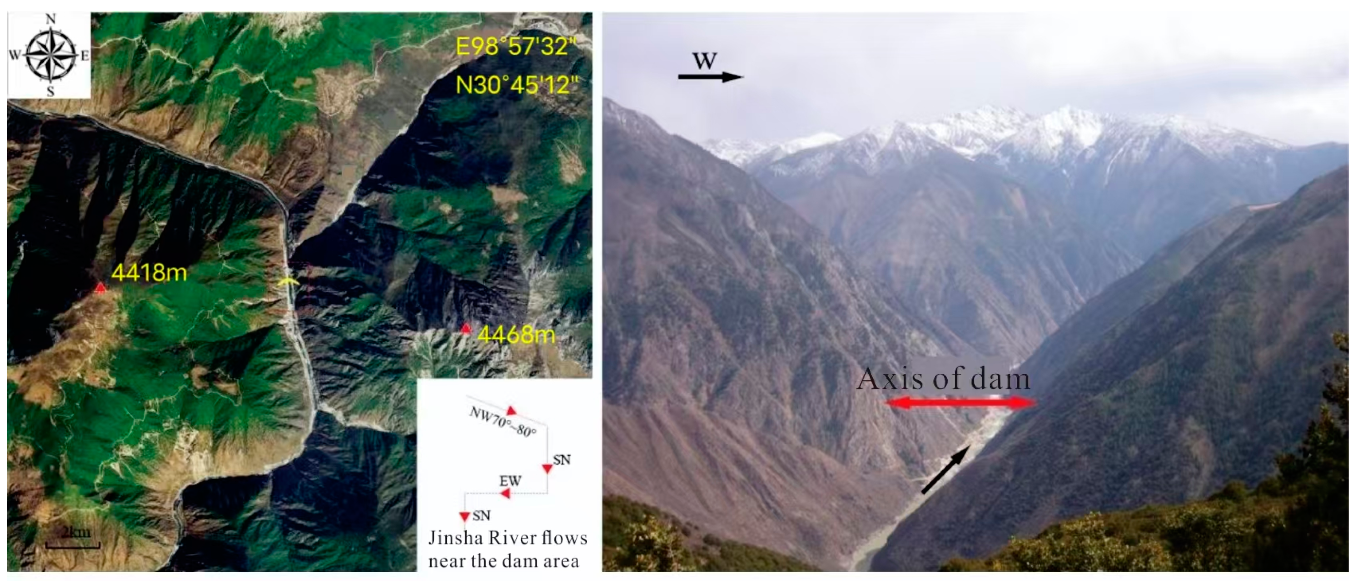
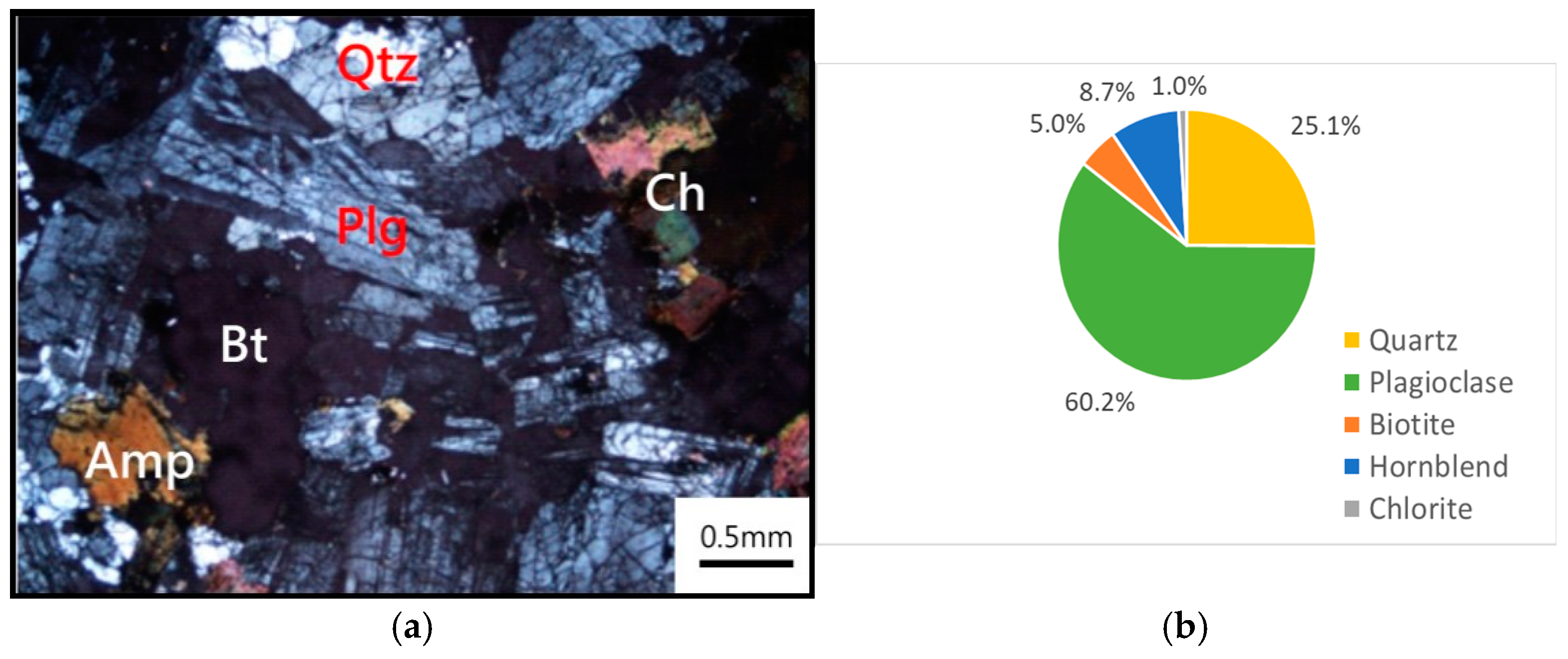
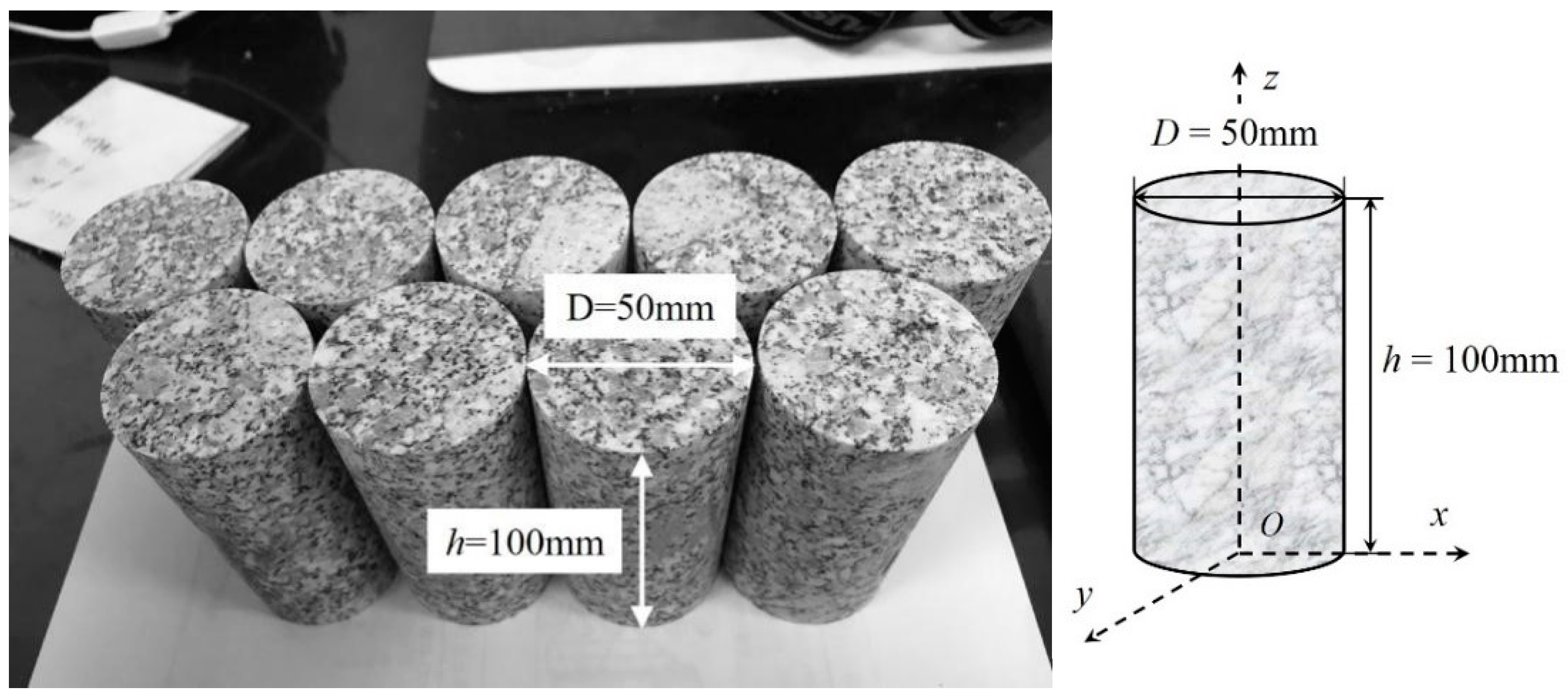
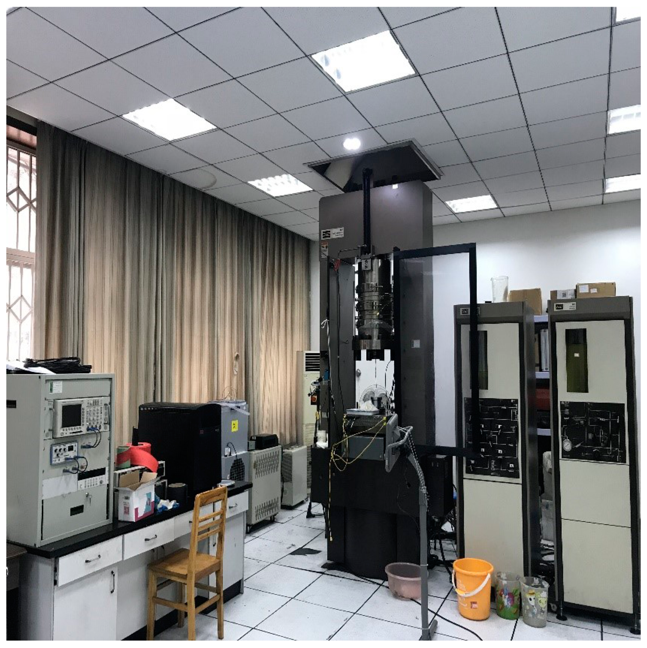
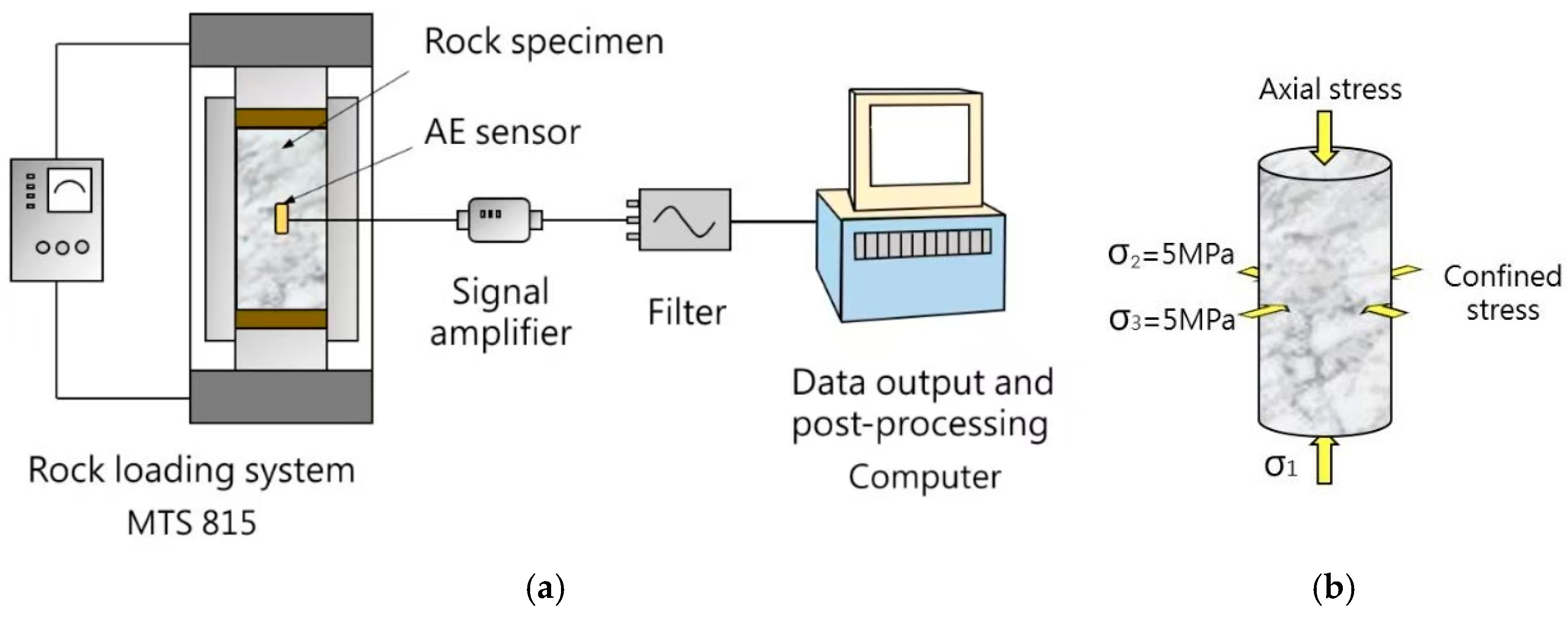
2.1. Samples and Test Equipment

The original rock samples were sourced from fresh rock at the Yebatan Hydropower Station dam site, situated 75 km west of Baiyu County in the upper reaches of the Jinsha River. The dam site is characterized by a deeply incised valley with steep slopes and narrow width, typical of a high mountain and deep valley topography (Figure 1). The tectonic and gravity stress superposition at the dam site has resulted in high initial ground stress, with a surrounding rock strength ratio of 4–5 and a maximum measured in-situ stress of 37.57 MPa. The rock samples are middle-acid intrusive granites of the Variscan Age (γδ₃⁴), exhibiting semi-idiomorphic fine-medium-fine granular and massive structures. Their main mineral components are plagioclase and quartz, which are generally hard and brittle, with a Mohs hardness of 6–7 and strong weathering resistance (Figure 2).

According to the current standard “Rock Test Regulations for Hydropower Engineering” (DL/T5368-2007 [39]), the diameter of the cylinder should be 48–54 mm, and the height-to-diameter ratio of the sample should be 2.0–2.5 mm. In this study, the rock blocks were processed into complete cylindrical samples according to this specification. The end diameter of the standard sample was D = 50 mm, and the height along the length was h = 100 mm. Some of the rock samples and their schematic diagrams are shown in Figure 3.

Rock triaxial acoustic emission tests were performed on an MTS815 rock testing machine(The MTS815 rock testing machine is manufactured by MTS Systems Corporation, which is headquartered in Eden Prairie, Minnesota, USA) at the Laboratory of Rock Mechanics, College of Water Resources and Hydropower, Sichuan University (Figure 4). The rock test system is composed of a loading system, a measuring system, and a controller. The acoustic emission system used for monitoring was the DiSP Acoustic Emission Test System, which has 16 channels. The test system mainly consisted of the following parts: an acoustic emission card (PC), an acoustic emission host system, an acoustic emission sensor, an acoustic emission preamplifier, and acoustic emission processing software.

2.2. Testing Program

The loading mode and stress path adhere to the test specifications outlined in the Engineering Rock Mass Test Method (GBT50266-2013 [40]) and the Rock Test Regulations of Hydropower and Water Conservancy Engineering (DL/T5368-2007), among others. The rock test procedure follows the steps illustrated in Figure 5.

Under hydrostatic pressure conditions with a predetermined confining pressure value of 5 MPa, the loading mode involves applying equal principal stresses σ₁ = σ₂ = σ₃. The loading rate for this process is set at 0.05 MPa/s.

The confining pressure on the rock sample is stabilized and maintained at a constant level. Subsequently, axial pressure is applied using stress control, with a loading rate of 1.0 MPa/s. The axial pressure, represented by σ₁, continuously increases until reaching 80% of the peak strength of the rock sample.

Once σ₁ has reached 80% of its peak strength, the load is applied through circumferential strain control at a loading rate of 0.02 mm/min. This process continues until the axial stress no longer decreases with increasing axial strain.

Throughout the entire testing process, synchronous acoustic emission monitoring was conducted simultaneously.

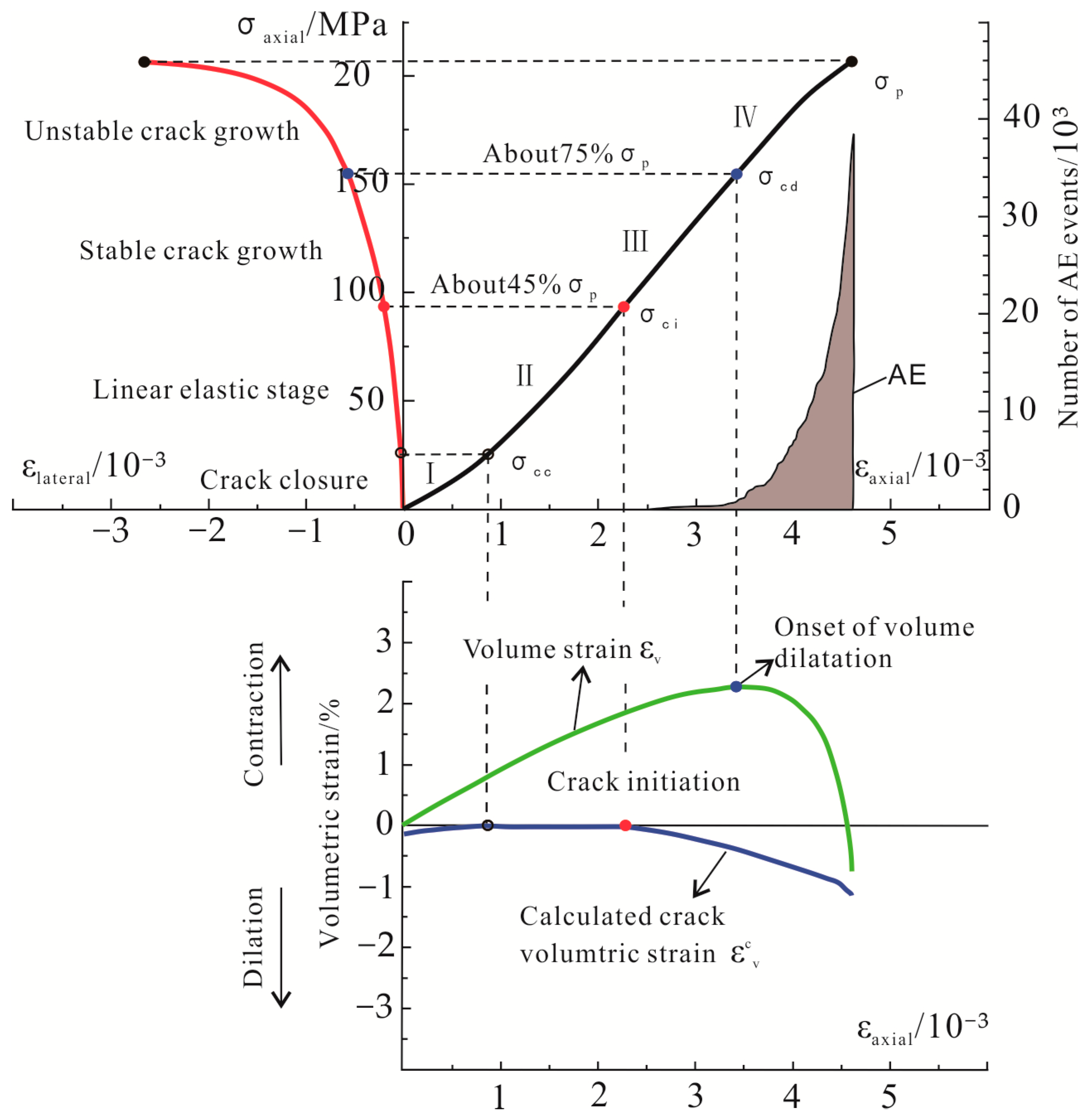
2.3. Test Results and Preliminary Analysis

We can obtain the stress–strain curve and cumulative quantity curve of the acoustic emission of granite according to the test results (Figure 5). This paper studies the stage before the peak stress of granite (σ_p = 205.96 MPa) and focuses on the microfracture of rock before failure; for example, the elastic modulus of granite is E = 5.40 × 10⁴ MPa, and Poisson’s ratio is µ = 0.120. Then, the volumetric strain and elastic volumetric strain of the rock can be calculated by the following:

$${\epsilon }_v={\epsilon }_v^e+{\epsilon }_v^c$$

(1)

$${\epsilon }_v={\epsilon }_x+{\epsilon }_y+{\epsilon }_z{\epsilon }_1+{\epsilon }_3$$

(2)

where ${\epsilon }_v$ is the volumetric strain, ${\epsilon }_v^e$ is the elastic volumetric strain, and ${\epsilon }_v^c$ is the crack volumetric strain. The volumetric strain consists of elastic volumetric strain and crack volumetric strain. The crack volumetric strain is caused by crack closure, initiation, and expansion. ε₁ is the axial strain, and ε₃ is the circumferential strain; in the test, ε₂ = ε₃. According to the generalized Hooke’s law, the crack volumetric strain can be calculated as follows:

$${\epsilon }_v^c={\epsilon }_v-{\displaystyle \frac{1-2\mu }{E}}\left({\sigma }_1+2{\sigma }_3\right)$$

(3)

where E is the elastic modulus of the granite and µ is Poisson’s ratio in this test. According to the calculation results, we obtain the relationship between the axial strain and other parameters.

The stress–strain curve before reaching the peak stress can be divided into several main stages according to the volumetric strain and crack volumetric strain: crack compaction, linear elastic deformation, stable crack growth, and unstable crack growth. The statistical results of the cumulative AE events reveal that the microfractures in the first two stages are relatively calm, but the number of microfractures in the fourth stage is very large. In particular, the number of microfractures increases sharply when the rock is near the peak stress before failure. At present, this feature is generally regarded as the precursor of rock fracture. The general characteristics of the AE or microfractures are shown in Figure 6. However, the behavior of microfractures cannot be statistically analyzed from the perspective of the stress–strain relationship and AE parameters.

3. Construction of the Rock Microfracture Network

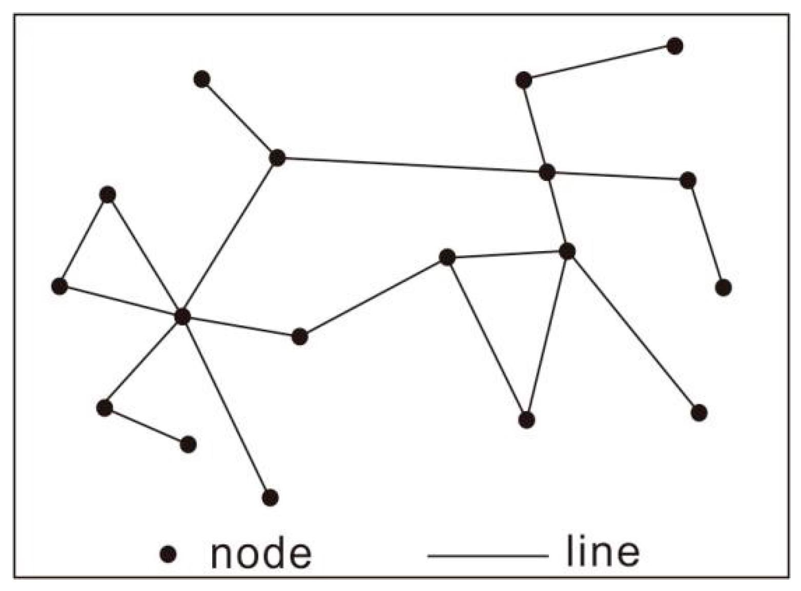
3.1. Introduction to Graph Theory and Complex Networks

Networks are ubiquitous in nature and human society, comprising nodes and links that connect them. These networks can represent individuals and their interconnections, whether they are tangible objects in Euclidean space, such as power grids, the internet, transportation networks, or neural networks, or abstract entities defined in conceptual space, such as social networks or collaborative networks in various industries, including research. Graph theory, a subdiscipline of discrete mathematics, serves as the primary method for studying networks. A fundamental natural definition of a graph is a set of points connected in some manner by a set of lines, as depicted in Figure 7.

All varieties of networks can be depicted by graphs, where nodes symbolize individual elements in the network, and edges denote deterministic relationships among connected elements. Thus, a network diagram can elucidate a system comprehensively via diverse individuals and connections. In this model, G represents the complex network, N is the set of nodes (rock fracture points), and K is the set of edges (interactions between fracture points). In general, complex network models can be expressed as follows:

$$\mathrm{G}=(\mathrm{N},\mathrm{K})$$

(4)

where N represents the set of network members (vertices or nodes) ≡{n1, n2, …, nN}; K represents the set of network member relationships (edges or connections), ≡{l1, l2, …, lN}. N = denotes the total number of complex network members (vertices or nodes), and any complex network graph can be represented by an N × N square connection matrix A:

$$A=\left[a_{ij}\right]=\left[\begin{array}{ccc}{a}_{11}& \mathrm{L}& a_{1N}\\ \mathrm{M}& \mathrm{O}& \mathrm{M}\\ a_{N1}& \mathrm{L}& a_{NN}\end{array}\right]$$

(5)

When there is a connecting edge between node i and node j, and I ≠ j, a_ij = 1; otherwise, a_ij = 0. Obviously, matrix A is a matrix of 01. For any i ∈ [1,N], a_ii = 0, this matrix helps in quantifying the interactions between nodes, where each element A ij indicates the presence or absence of a connection. It is more convenient and faster to calculate network parameters in batches by representing the network by a matrix.

3.2. Basic Parameters of Complex Networks

The fundamental physical parameters of networks include degree, shortest path, clustering coefficient, between centrality, and more. The dynamic evolution of a network can be measured by observing changes in these characteristic parameters. Typically, the basic physical quantities of complex networks include the following items.

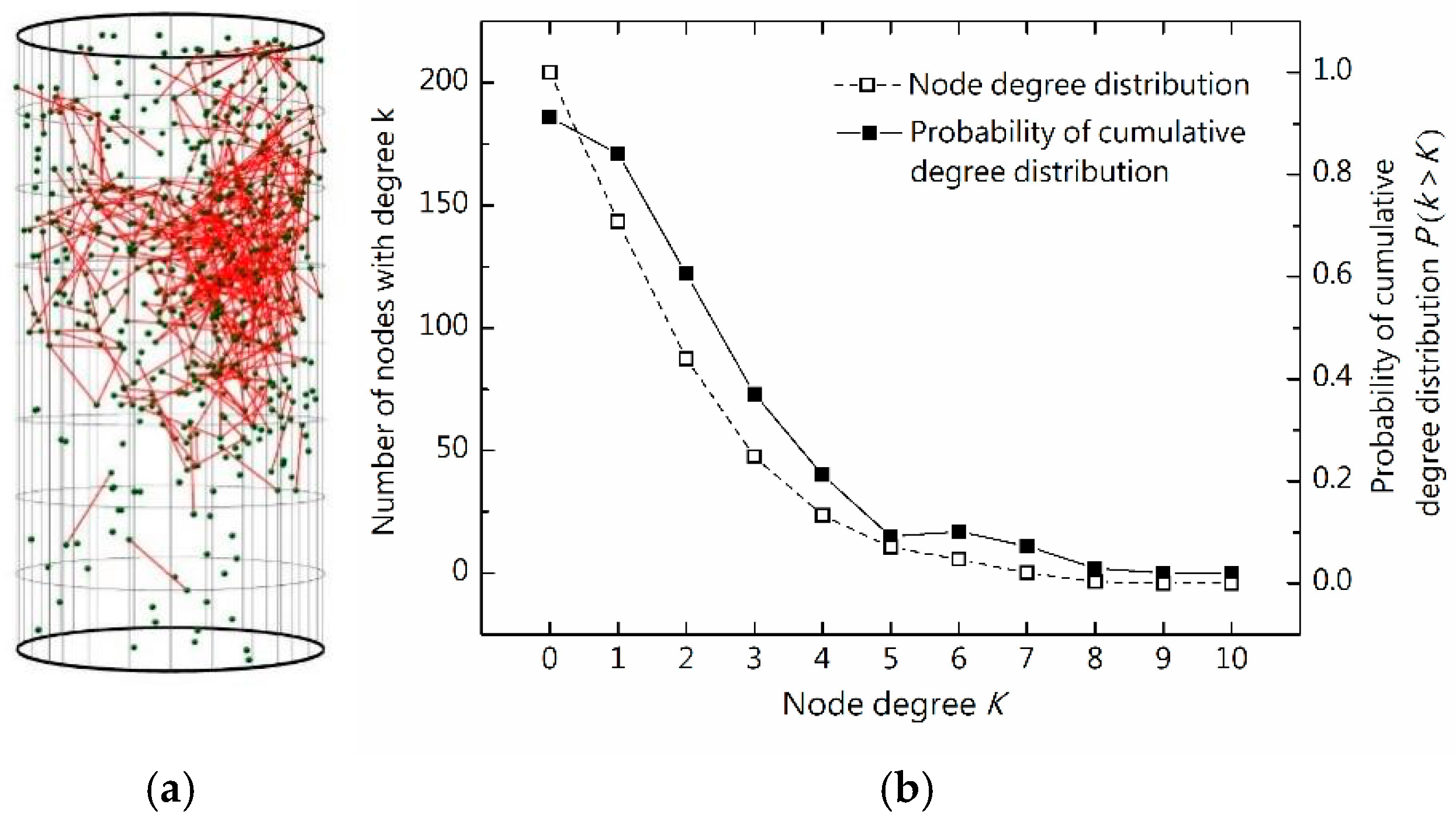
3.2.1. Degree and Degree Distributions

The node degree refers to the count of edges directly linked to a node, indicating the number of other nodes directly connected to it, denoted as k. The degree distribution elucidates the statistical distribution of degrees across all nodes in the network, expressed as p(k). p(k) also represents the likelihood that any node’s degree equals k under the random consistency principle. The node degree serves to illustrate the communication capacity and resource utilization of individual network members, and it can also reveal the scale-free characteristics of complex networks [24]. The degree k_i of any node i in the network can be calculated using the connection matrix according to Equation (6). The degree k_i quantifies the number of direct connections node i has within the network.

$$k_i=\sum _{j=1}^n a_{ij}$$

(6)

The average degree of all nodes in the network was calculated according to Equation (7) <k>, the average degree provides a measure of the overall connectivity within the network.

$$⟨k⟩={\displaystyle \frac{1}{n}}\sum _{j=1}^n k_i$$

(7)

3.2.2. Shortest Path

The shortest path is the number of edges that connect the shortest distance between two nodes i and j, expressed by d_ij. The average shortest path refers to the average of the shortest paths between all points and other points, which can represent the connectivity of the network and is represented by L. The average shortest path L of the complex network can be calculated through the connection matrix A according to Equation (8):

$$L={\displaystyle \frac{1}{N(N-1)}}\sum _{i,j\in N,i\ne j} d_{ij}$$

(8)

3.2.3. Clustering Efficiency

Clustering efficiency, denoted by c, represents the clustering of nodes within a network. k_i denotes the degree of node i, indicating the number of edges connected to it. Thus, node i can potentially have k_i (K_I − 1)/2 edges with other nodes. However, in reality, there are only e_i edges among these k_i nodes. The clustering coefficient c_i of node i is calculated as the ratio of the actual number of edges e_i to the maximum possible number of edges k_i (K_I − 1)/2, as follows:

$$c_i={\displaystyle \frac{2e_i}{k_i\left(k_i+1\right)}}$$

(9)

The matrix calculation can be expressed as Equation (10):

$$c_i={\displaystyle \frac{\sum _{j,m} a_{ij}{a}_{jm}{a}_{mi}}{k_i\left(k_i+1\right)}}={\displaystyle \frac{\sum _{j=1}^n \sum _{m=1}^n a_{ij}{a}_{jm}{a}_{mi}}{k_i\left(k_i+1\right)}}$$

(10)

The average clustering efficiency of the network is calculated according to Equation (11):

$$⟨c⟩={\displaystyle \frac{1}{n}}\sum _{j=1}^n c_i$$

(11)

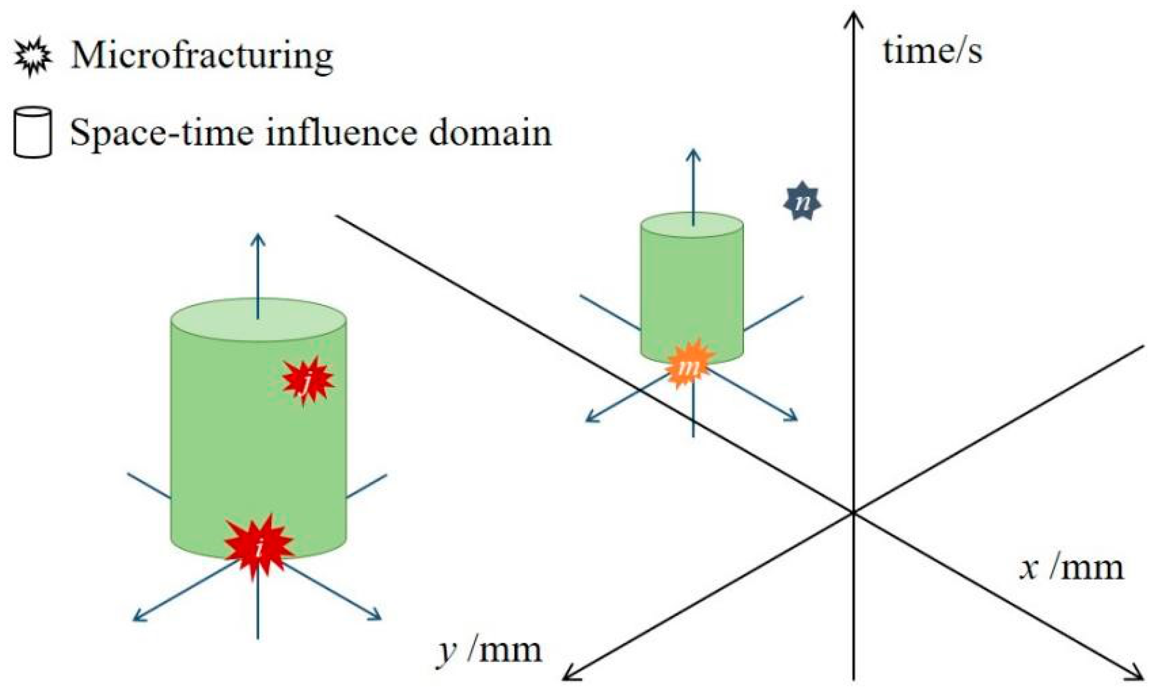
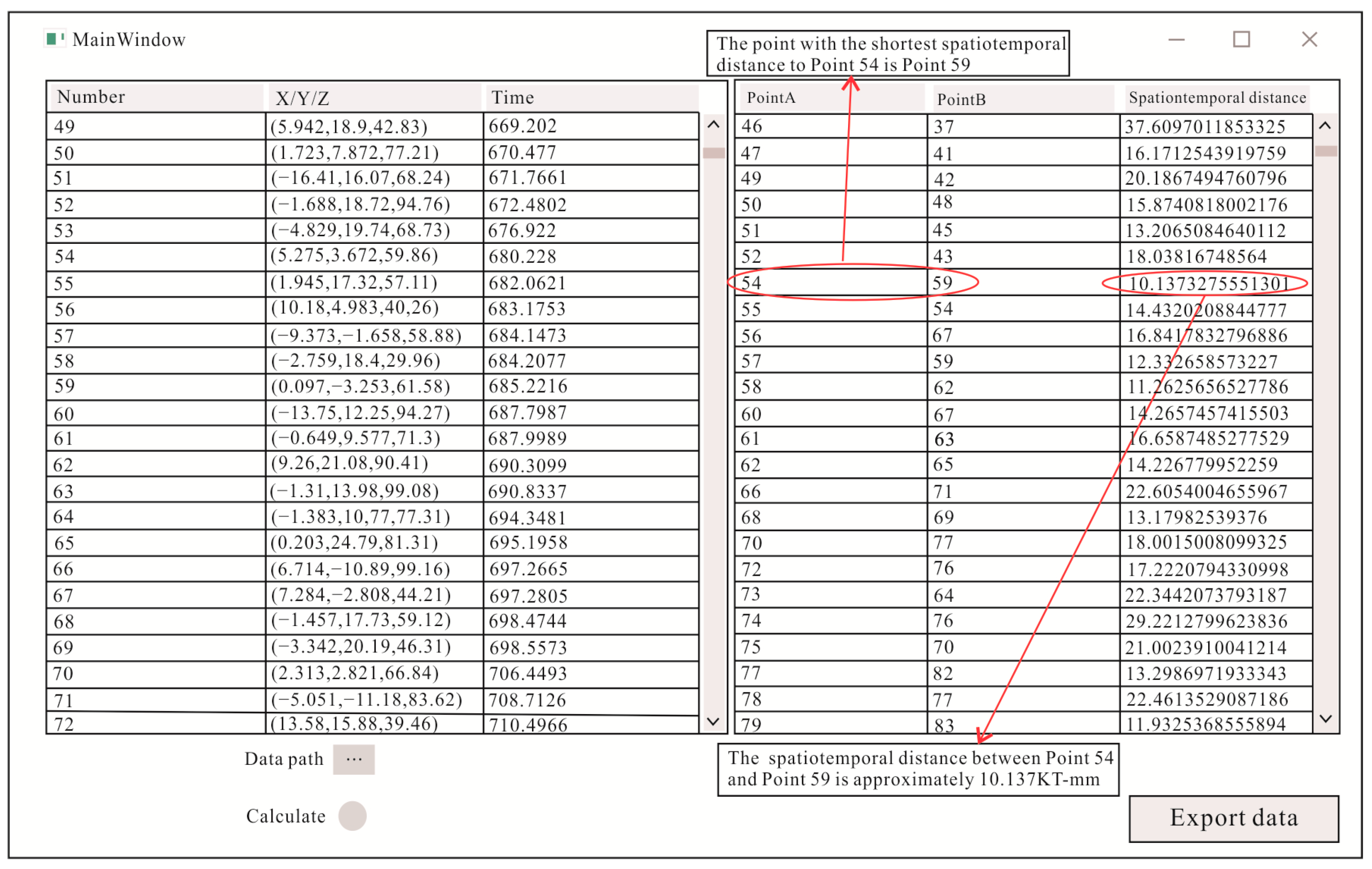
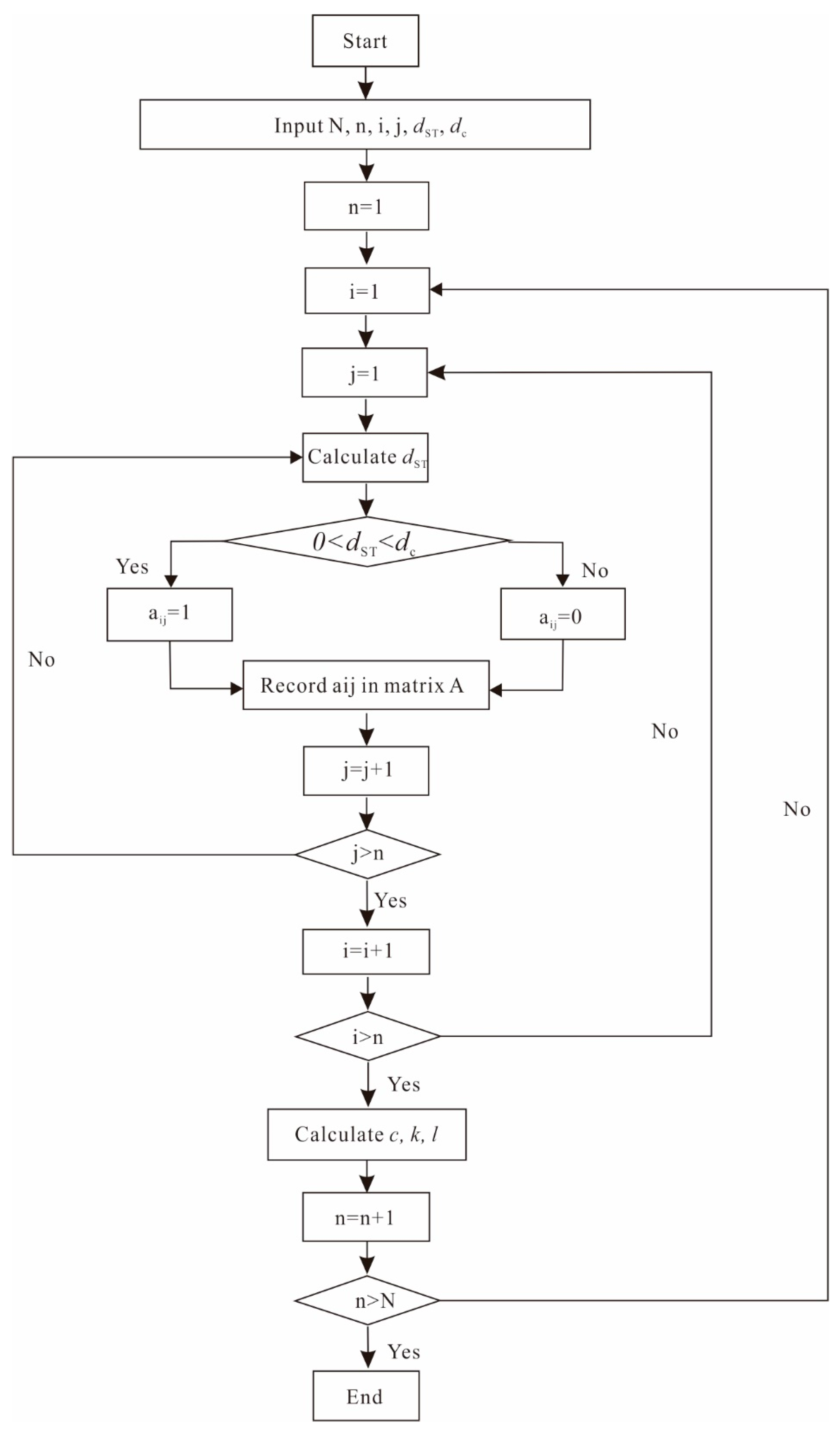
3.3. Space–Time Single-Link Cluster

The single-link group method is commonly employed in seismology to evaluate the spatial clustering characteristics of vibrations. Currently, this method involves identifying the closest source point to each seismic starting point in space, connecting edges between them to form a single-link, and ultimately constructing a focal event sequence within a defined region comprising points and single-links. However, it is evident that earthquake occurrence is not solely determined by spatial proximity. For example, in the analysis of major earthquakes, despite the Diexi and Wenchuan earthquakes being about 100 km apart, their incidence spans over 74 years, with no established connection between them. Thus, when examining rock fracture properties, relying solely on spatial distance to calculate single-links inadequately captures the correlation between fracture points. According to space–time window theory [41], the occurrence of earthquake aftershocks is closely related to both space and time. Similarly, in the study of rock fractures, the occurrence of subsequent microfractures is affected by the spatiotemporal properties of the previous microfractures.

Space–time single-link clustering is one such method for calculating the temporal and spatial clustering of earthquakes [42]. This method involves adding a time factor to the construction of a single-link group, determining the shortest space–time bond length between each break point by solving the time-space distance, and calculating the cluster attribute of the break point (Space–time single-link group theory (Figure 8)). A possible microrupture event i has a certain influence region in both time and space. For example, rupture point j is within the influence range of rupture i in both time and space, so microruptures i and j are correlated, whereas microrupture events m and n are not correlated.)

The structure of the microfracture spatiotemporal single-link group is established. In the process of rock deformation and failure, the most basic properties of microfracture events are the occurrence time and spatial coordinates, both of which can be directly obtained through rock acoustic emission positioning tests.

The spatiotemporal coordinates i (xi, yi, zi, ti) of any AE break point can be obtained according to the AE location test data. The time interval tij and the space distance dij (i ≠ j; i, j ∈ [1, n], where n is the total number of break points) (

Table 1. AE location test data.

(n)	x	y	z	Time
i	xi	yi	zi	ti
j	xj	yj	zj	tj
…	…	…	…	…

):

$$t_{ij}=t_j-t_i$$

(12)

$$d_{ij}=\sqrt{{\left(x_j-x_i\right)}^2+{\left(y_j-y_i\right)}^2+{\left(z_j-z_i\right)}^2}$$

(13)

The space–time bond length d_ST is the space–time distance between any two rupture events, which can be obtained by the time interval tij and spatial distance dij between the two rupture points [42]:

$$d_{ST}=\sqrt{d_{ij}^2+C\cdot t_{ij}^2}$$

(14)

where d_ST is the spatiotemporal distance between two acoustic emission events in mm ST; d_ij is the distance between two acoustic emission events, in mm; C is the spatiotemporal correlation constant, 1 mm·s^–1, is taken according to the relevant literature on seismology; t_ij is the time interval between two acoustic emission events, in s.

For any event in the microrupture event sequence [1, n], if the time series number of the event is m, then the spatiotemporal distance between the event and all other events can form a disordered finite set M = {dm1, dm2, dm3, …, dmn}. If the smallest element in the set M is dmn, then event n is the event with the shortest space–time distance from event m, and a space–time single-link is established between event m and event n; that is, dmn = min {dm1, dm2, dm3, …, dmn}. Through the above method, the spatiotemporal single-links between all microfracture points in the process of rock deformation and failure can be obtained, and the ST-SLC single-link group framework of rock failure can be constructed.

By writing a program in MATLAB 2019a (The software version number for MATLAB 2019a is R2019a), one can import the acoustic emission test data of the rock with a single command. After the value of the spatiotemporal correlation constant C is input and the “Calculate” button is clicked, the computational results of the spatiotemporal single-link group are exported, as shown in Figure 9.

On the basis of the analysis results of the spatiotemporal single-link group, the single-link connection status of any microfracture point can be obtained. For example, the point with the shortest spatiotemporal distance to point 54 is point 59, and the spatiotemporal distance between them is about 10.138 mm. Each microfracture point is clearly connected by at least one spatiotemporal single-link.

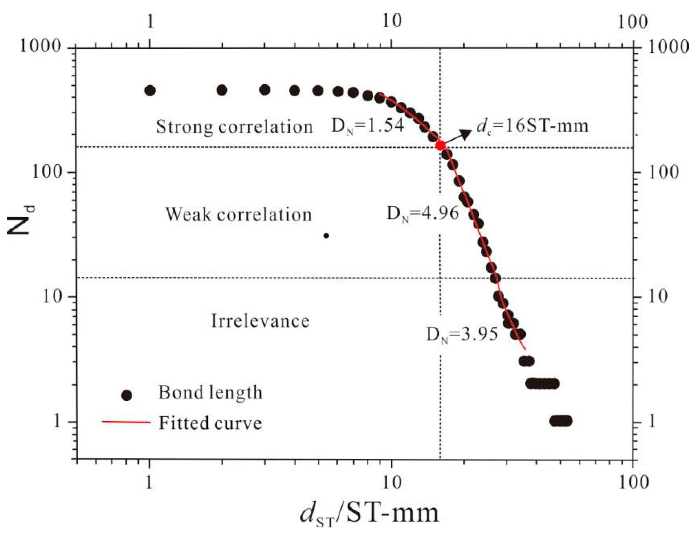
3.4. Solution of the Characteristic Bond Length d_c

In the investigation of spatiotemporal single-link group architecture (ST-SLC), the presence of discrete break points led to the emergence of single-links with notably large spatiotemporal distance values within the spatiotemporal single-link group. Such single links, however, fail to accurately represent the true correlation properties between two points and should, therefore, be discarded. This paper introduces an eigenvalue to measure the correlation of microbreak points, termed the eigenbond length (d_c), which signifies the spatiotemporal distance of rock microbreak points. When the spatiotemporal single-link length (d_ST) exceeds the characteristic bond length (d_c), the “time-space bond” between the two break points lacks practical significance, suggesting either no correlation or a very weak correlation between the two points. Conversely, when the bond length (d_ST) between the microbreak points is less than the characteristic bond length (d_c), there is a meaningful “space–time bond” between the two break points, indicating a strong correlation between them.

By calculating the spatiotemporal distance between any two adjacent points in the framework of the spatiotemporal single-link group, the spatiotemporal bond length-frequency relationship can be obtained, and the spatiotemporal bond length-d_ST-bond long frequency distribution relationship N_d can be further obtained.

According to fractal theory in mathematics, the relationship between the length and number of space–time bonds exhibits local scale-free characteristics. Within the scale-free region, the distribution of spatiotemporal bond lengths within the ST-SLC framework demonstrates a fractal structure, with its slope representing the fractal dimension (D_N). Similarly, the bond length-frequency relation also has the same fractal dimension (D_N), which can be divided into scale-free intervals with self-similarity. For example, in geotechnical or geological fields, the same D_N typically indicates the self-similarity of faults, geological structures, and other seismic events [43].

The fractal dimension can be determined by calculating the slope of the logarithmic curve of the spatiotemporal bond length and bond length frequency, as defined by Equation (15). The scale-free regions within the spatiotemporal single-link group framework can subsequently be delineated on the basis of various fractal dimensions.

$${\mathrm{D}}_{\mathrm{N}}=-\underset{d\to 0}{\lim }{\displaystyle \frac{\ln {\mathrm{N}}_{\mathrm{d}}}{\ln d}}$$

(15)

where D_N is the frequency-key length fractal dimension; d is the spacetime distance between two break points, that is, the length of the spacetime bond, in ST-mm

The N_d–ST-SLC architecture is the number of single-link frequencies in which the key is longer than d.

Following the processing of granite acoustic emission test data, the spatial and temporal single-link group framework for each sample is derived. In accordance with the aforementioned theory, the structure of rock single-link groups is analyzed, and the fractal dimension (D_N) is determined by fitting different scaling segments of the logarithmic curve of spatial and temporal bond length d_ST-bond length frequency N_d, as depicted in Figure 10. Each scale-free interval can then be categorized on the basis of different values of D_N, enabling the resolution of feature key lengths. When d_ST ≤ 16ST mm, the fractal dimension D_N ≈ 1.54; conversely, when d_ST > 16ST mm, a significant change occurs, with the fractal dimension D_N ≈ 4.96. At this juncture, d_ST = 16ST mm serves as a pivotal point for discerning shifts in the frequency distribution of key lengths, denoting the characteristic key length (d_c) as 16ST mm. Moreover, for enhanced clarity, the natural logarithm with base e can be replaced by the logarithm with base 10, yielding identical results, as per the base-change formula of the logarithmic function.

When it is challenging to directly discern the turning point of the aforementioned curve, a slope change curve can be derived by differentiating the function (Figure 11). By examining dlnd_ST/dlnnd-d_ST, it becomes evident that the number distribution of spatiotemporal bond lengths undergoes a change. Similarly, the d_ST-N_d logarithmic curve notably changes when d_ST = 16ST mm. Once the characteristic bond length is established, the correlation properties of all the acoustic emission points are determined based on the relationship between d_ST and d_c of each spatiotemporal bond length within the spatiotemporal ST-SLC framework. This serves as the foundation for constructing the intricate rock fracture network in subsequent steps.

3.5. Construction Method of the Rock Microfracture Network

The process of rock failure arises from the propagation and penetration of macroscopic cracks initiated by microfractures. Acoustic emission technology enables the monitoring of fundamental properties associated with all microfracture events in this process. By conceptualizing rock microfracture points as nodes within a network and considering the interactions between these fracture points as interconnected edges, all the acoustic emission points from rock fractures can form a network comprising numerous nodes and edges. Moreover, the network at various stages throughout the rock fracture process can be viewed as a dynamic complex network that undergoes temporal changes.

By utilizing the temporal and spatial characteristics of acoustic emission events, the length of the spatiotemporal bond between fracture points is determined, and the correlation property of fracture points is inferred based on small spatiotemporal bond lengths. The rock fracture network model is then established through MATLAB matrix operations. The edge construction method involves the following steps: if the spatiotemporal distance between any two points is less than the characteristic bond length, it is concluded that the two fracture points are correlated; thus, an edge is added between them. Conversely, if there is no correlation between two points, no edge is added. The network construction process is outlined as follows.

At the onset, there exists an initial isolated acoustic emission point. Upon adding a second point to the network, the spatiotemporal distance d₁₂ = [(x₂ − x₁)² + (y₂ − y₁)² + (z₂ − z₁)² + C (t₂ − t₁)²]^1/2 is computed to determine if d₁₂ is less than or equal to the characteristic bond length d_c. If true, an edge is added between the first point and the second point, and the value d₁₂ = d₂₁ = 1 is recorded in the 2 × 2 matrix. Conversely, if no edge is added, the value d₁₂ = d₂₁ = 0 is recorded in the matrix.

Once the number of nodes N ≥ 2, each subsequent acoustic emission point m is added. The spatiotemporal distance dmn between this new point and all existing acoustic emission points is computed (1 ≤ n < N, where N represents the total number of nodes). By assessing the relationship between dmn and the characteristic bond length d_c, the connectivity of node m with any node n is determined. Similarly, when nodes m and n are connected, a_mn = 1; otherwise, a_mn = 0.

With each addition of a node, the connection matrix A = {a_ij} expands by one order, and correspondingly, the network composed of acoustic emission points and its physical attributes undergoes changes. The outcome is a network comprising all the sound emission points and edges, constituting the complex network model of rock fracture. The complex network of rock failure dynamically evolves with the progression of rock deformation and failure. The network flowchart illustrates the modeling process (Figure 12).

There are 637 AE data points in sample GC1 before the peak, and a network model with all nodes and different numbers of edges (determined by the length of the characteristic key) can be constructed. By calculating whether there is an edge between any two nodes, the network model diagram corresponding to any loading time can be constructed with the help of the DataViewer3D data visualization tool (Figure 13). According to the solution of the network parameters, the dynamic evolution process of rock fracture development can be described.

4. Results and Discussion

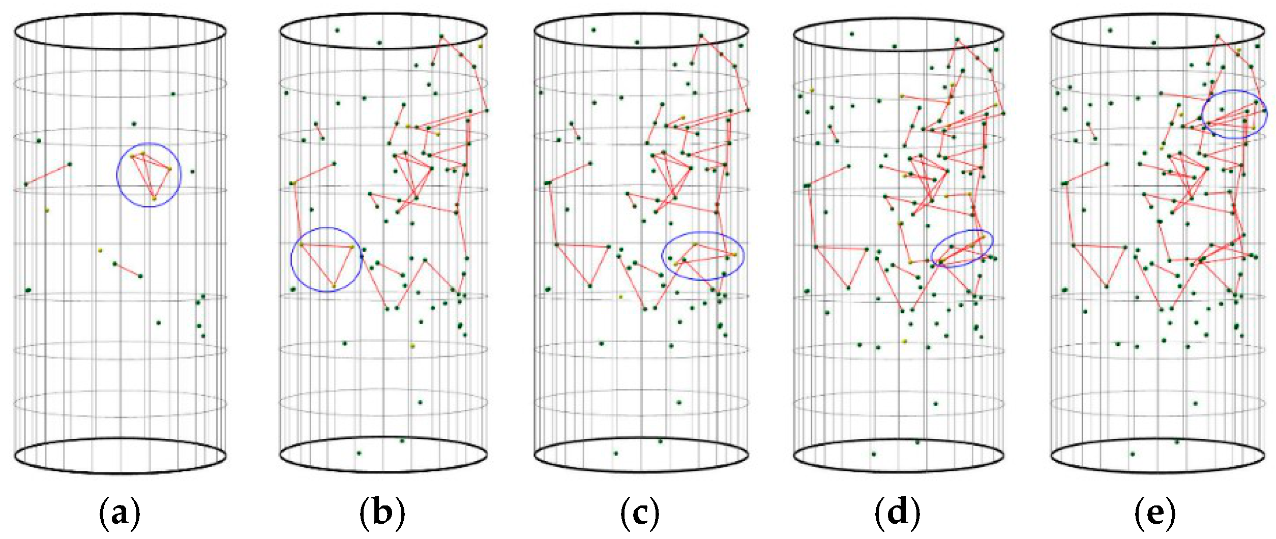
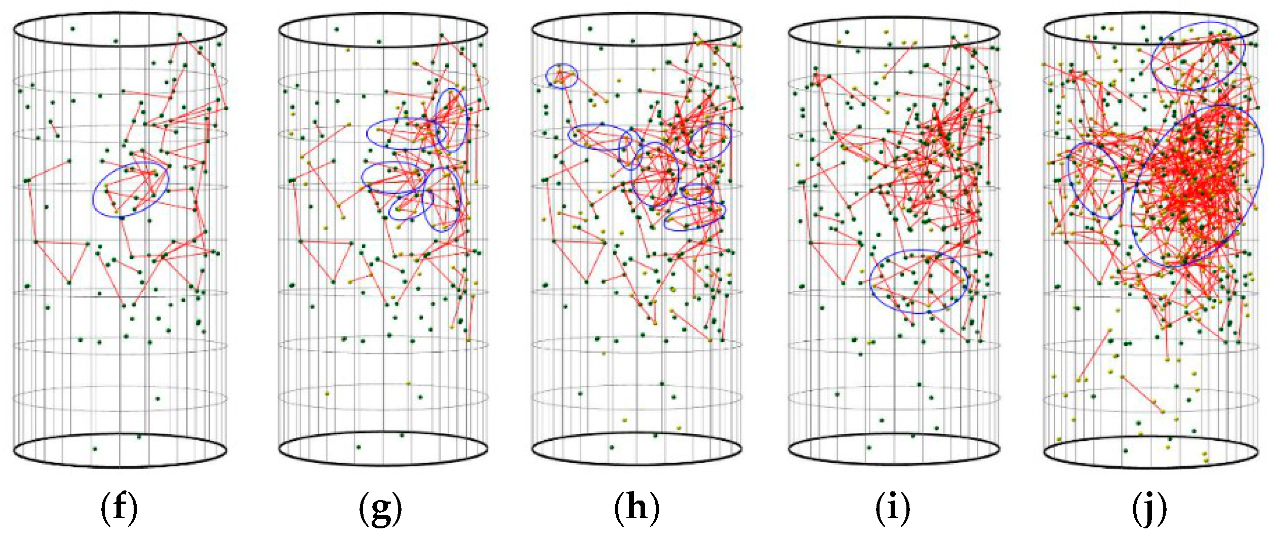
4.1. Characteristics of Rock Microfracture Networks

Numerous research findings indicate that real networks typically exhibit the following characteristics [44]: (1) Statistical behavior: Networks with many nodes often display certain statistical properties. (2) Sparsity of connections: Most networks feature numerous nodes with sparse connections. (3) Uncertainty of connections: Connections within networks tend to lie between complete regularity and randomness. (4) Complexity of dynamic behavior: Each node within the network demonstrates nonlinear dynamic behaviors such as bifurcation and chaos. Space–time evolution: The evolution of networks over space and time manifests rich and complex dynamic behaviors. Generally, research on network models concentrates on examining some of these characteristics.

This study focuses on the fracture point network at peak stress, aiming to analyze the distribution pattern of node degrees within the sample and validate the characteristics of the rock fracture network. Based on the aforementioned analysis, rupture points situated at excessively long temporal and spatial distances from other points can be deemed isolated rupture points. These rupture points are discrete and have a degree of 0. Conversely, a few fracture points serve as pivotal nodes facilitating crack propagation, exhibiting a “Hub” function by connecting multiple microcracks. These fracture points demonstrate high clustering with other points and consequently exhibit a significantly large degree of connectivity.

In the fracture point network of sample GC1 under peak stress, the average node degree is 1.67, with the highest node degree recorded at 8. Specifically, 2 nodes exhibit a degree of 8, whereas 11 nodes have a degree of 7, collectively accounting for about 2% of the total fracture points. Moreover, a significant portion of the nodes (479) have a degree less than or equal to 2, accounting for more than 75% of the total. Overall, most rupture points show small degrees, indicative of the “extension type” or isolated category, whereas a minority exhibit high degrees, representing core nodes generated by “aggregation”. As shown in Figure 14, both the number of nodes and the cumulative distribution probability decrease consistently with increasing degree, with the rate of decrease gradually diminishing. This pattern aligns with a power-law distribution (f(x) = X^–α, (α > 0)), highlighting the scale-free properties characteristic of a typical complex network [36].

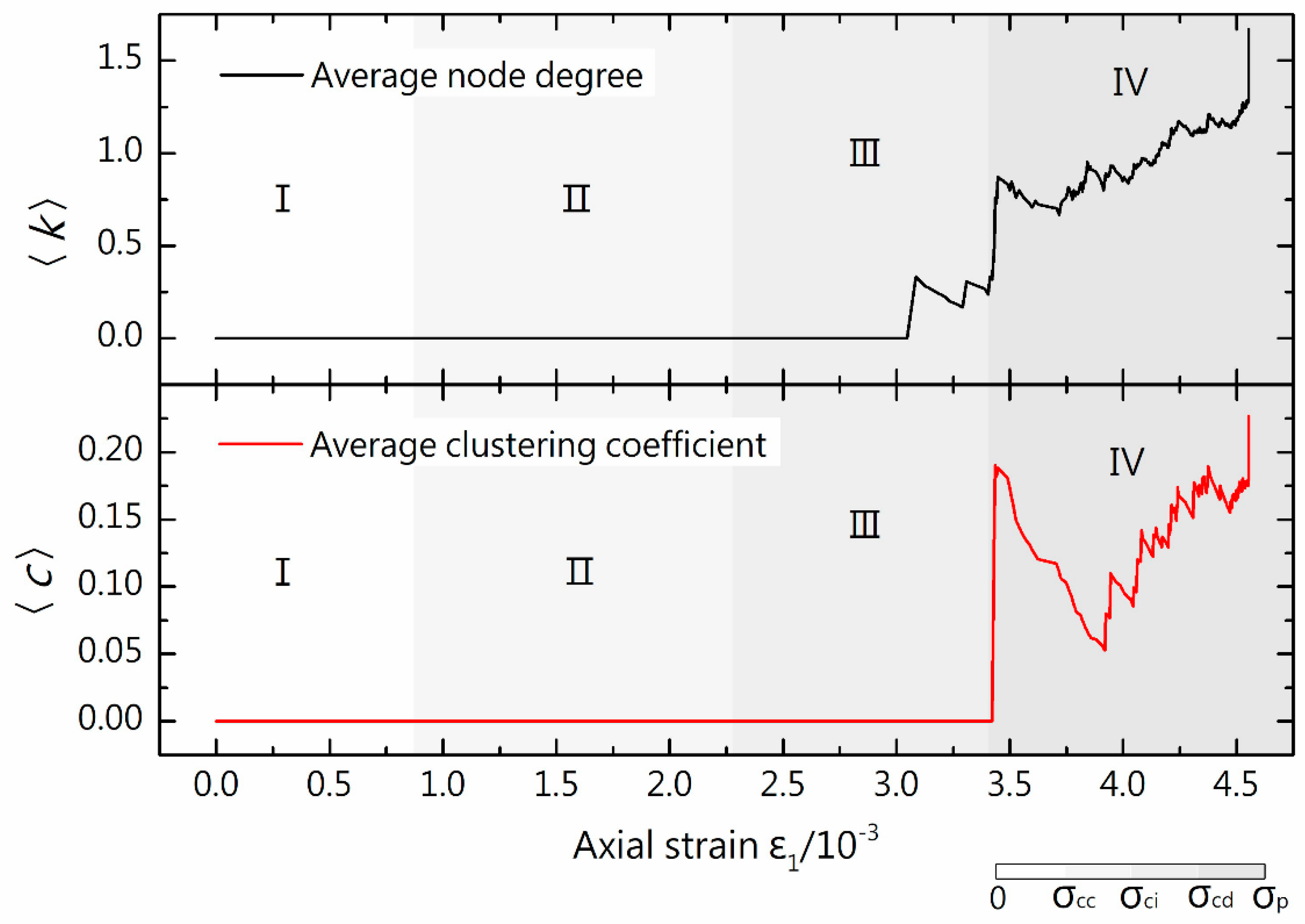
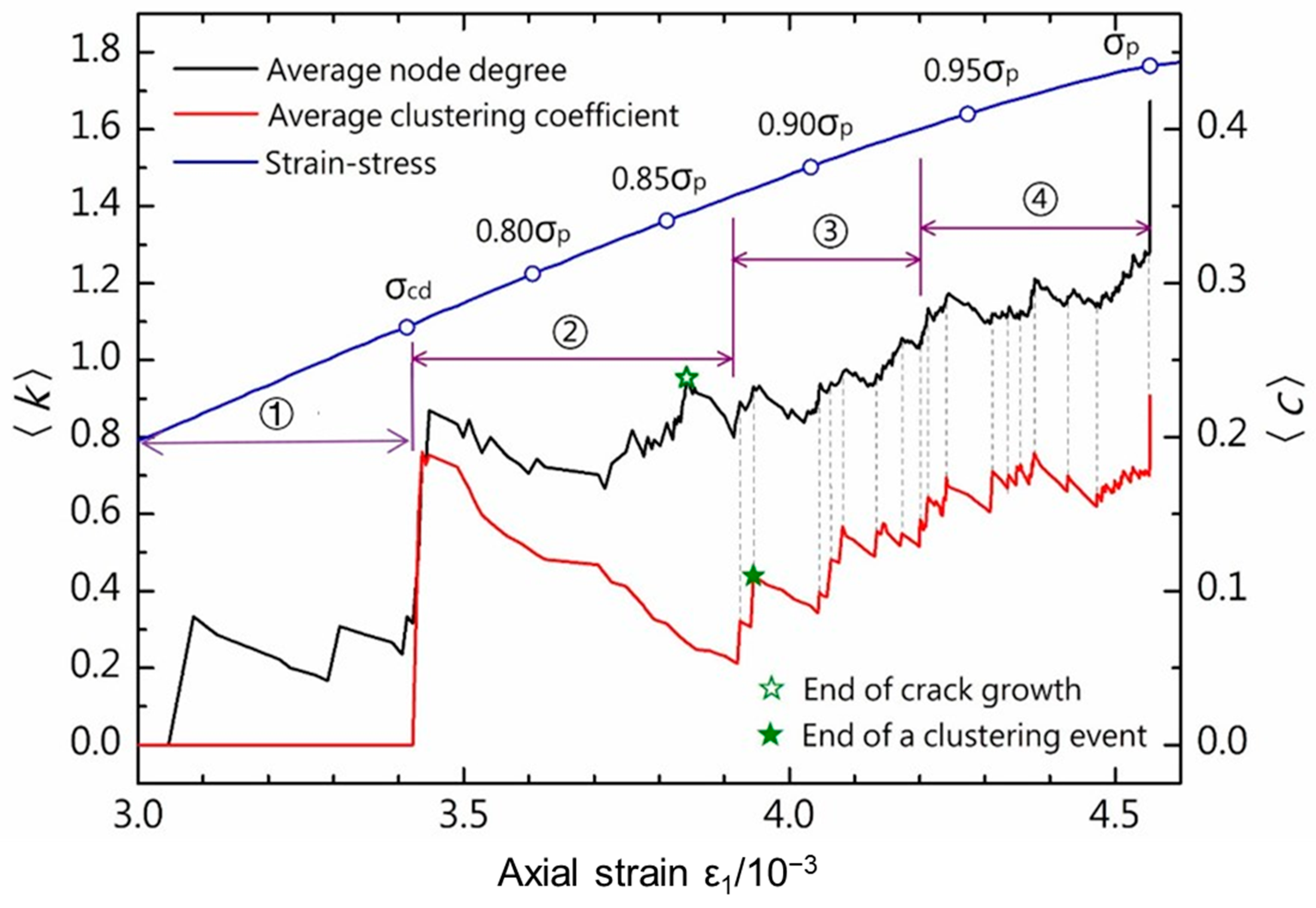
4.2. Dynamic Evolution Characteristics of the Rock Microfracture Network

Any real network is time-dependent. Combined with the theory of network dynamics, the evolving microfracture network can more accurately represent the change in rock microfracture activity. We choose two notations, the average degree <k> and the average clustering coefficient <c>, to describe the properties of the microfracture network. Through the changes in <k> and <c>, the specific process of rock fracture can be analyzed from the perspective of network evolution.

<k> and <c> can be solved via Equations (6) and (11).

According to the definition of network notations, the node degree is the connected edges of the nodes, which indicates that one fracture event can affect other events in the network; the clustering coefficient describes the clustering degree of nodes, which indicates the aggregation property of microfractures in the network. Several simple graphs are used to illustrate the relationship between network evolution and changes in two characteristic parameters (

Table 2. Change in notations when the two-node network becomes a three-node network (In the table, the black circle represents the fracturing point, and the short red segment represents the correlation between the fracturing points).

Network Graph (2 Nodes)	Notations	Evolved Network Graph (3 Nodes)	Notations
	<k> = 0, <c> = 0		<k> = 0, <c> = 0
			<k> = 0.67, <c> = 0
			<k> = 1.33, <c> = 0
	<k> = 1, <c> = 0		<k> = 0.67, <c> = 0
			<k> = 1.33, <c> = 0
			<k> = 2, <c> = 1

).

In the fracture point network, there are only two types of relationships between any two fracture points: either they are related or they are unrelated. When a fracture point is isolated, its node degree is 0, resulting in an average degree of 0. Conversely, when two fracture points are related, the degree of both nodes is 1, yielding an average degree of 1. Upon the occurrence of a third fracture point, three possible relationships emerge between the third fracture point and the first two fracture points: (1) related to both, (2) unrelated to both, and (3) related to one of them. Hence, there are four possible outcomes in total. Notably, the increase in the average degree is associated with the interrelatedness of the fracture points, indicating the connection of microfractures or the propagation of microcracks within the network. On the other hand, the increase in the clustering coefficient is solely linked to the presence of closed loops, which is indicative of the rapid occurrence of continuous fracture events over a short time and distance or the aggregation of microfractures.

As deduced from the preceding analysis, the alterations in notations effectively capture the evolution behavior of the microfracture network. Furthermore, the characteristic parameters of the network at any given time can be computed utilizing the parameters recorded by the acoustic emission sensor (Figure 15).

During the early and middle stages of the loading test, microfractures in the rock manifested in a random manner, exhibiting strong discreteness, with no evident correlation between fracture points. Consequently, both the average degree and average clustering coefficient of the microfracture network remain at 0 during this period. This scenario persists until the middle stage of stable crack growth. As microcracks continue to proliferate, the average values undergo a sudden increase. However, the appearance of random isolated fracture points subsequently causes a decrease in the average value. During this phase, characterized by relatively stable and slow crack growth, there is no aggregation; therefore, the average clustering coefficient remains unchanged and equals 0. As the deformation of a sample approaches the expansion point, the rate of microcrack initiation and growth experiences a sudden surge, leading to sudden clustering. Consequently, both the average clustering coefficient and average degree undergo a sudden increase to very high levels. In the stage of unstable crack growth, <k> and <c> increase and decrease repeatedly, but in general, they increase.

4.3. Analysis of Microfracture Activity

To explain the behavior of microfractures in detail, we separate the changing part of the curve and establish a model of the microfracture network at multiple times in this stage.

Apart from the peak value observed in the average clustering coefficient curve, each microfracture clustering event is also associated with a noticeable peak value on the average degree curve. As microcracks begin to cluster, the deformation of the rock transitions into an unstable crack growth stage. Subsequently, microcracks continue to propagate, expand, cluster, overlap, and exhibit other behaviors. Overall, on the basis of the variation patterns of the average degree and average clustering coefficient of microfractures, the microfracture process of granite can be divided into four main stages, as depicted in Figure 16.

Silence period (75%σ_p): During the compaction stage (I) and linear elastic stage (II) of the granite sample, as well as the initial and middle stages of the stable crack growth stage (III), acoustic emission events are rare and discrete. The occurrence of fracture points is highly random, with only a few appearing sporadically. As the sample approaches the expansion point, localized finite expansion occurs at the fracture points, leading to the formation of random microcracks.

Microcrack growth period (75%σ_p to 87%σ_p): During the transition from the stable crack growth stage to the unstable crack growth stage, there is a localized expansion of microcracks within the rock. This leads to a notable aggregation event of microcracks. Concurrently, the volumetric strain of the granite increases, causing the rock volume to shift from contraction to dilation, indicating the onset of the unstable crack growth stage. During this period, the primary activity of microfractures was expansion and continuation. The average degree of the microfracture network continuously fluctuates, indicating that fracture points in the rock appear randomly and are related to each other. Additionally, the average clustering coefficient of the network only exhibits a few maximum values (2 times), suggesting that microfractures in the rock experience limited aggregation events. Therefore, in the early stage of unstable crack growth, the main activity of microfractures is connectivity propagation.

The cluster increasing period (87%σ_p to 95%σ_p): When microcracks expand to a certain extent, because of damage accumulation, the sum of the dissipated energy released by stable crack growth and the elastic strain energy stored by rock deformation is not enough to meet the mechanical energy absorbed by the rock, and more microcracks occur in the rock interior faster. Faster and more microfractures exhibit more obvious aggregation. During this period, the activity of microfractures is more obvious than that in the previous stage, and clustering events mainly occur around the initial clustering events. According to the previous analysis, the clustering of nodes can greatly improve the average value of nodes. Therefore, owing to the occurrence of random fractures and expansion, the average degree of the microfracture network will fluctuate, and with increasing strain, the microfracture aggregation will increase, and the average degree will increase overall. In summary, the behavior of microcracks changes to rapid growth and local aggregation.

Centralized clustering and overlapping period (after 95%σ_p to after σ_p): As several distinct local aggregations of microcracks occur, the internal damage within the rock accumulates to a very high level. During this phase, due to significant aggregation events, the average degree of the microcrack network increases to a relatively high level. Additionally, the average clustering coefficient decreases but more intensively changes, indicating a reduction in isolated microcrack events and an increase in cracks with rapid growth and microfracture clustering events. During this period, microcracks cluster more intensively, primarily concentrated near the final fracture surface. As the peak value approaches, the average clustering coefficient experiences an exponential increase, indicating that many microcracks cluster together, extensive crack interactions, rapid crack expansion, and rock near failure.

The aforementioned behaviors of microfractures are directly observable from the network diagram (Figure 17). The small ball marks the location of the microfracture, the yellow ball marks the location of the recent microfracture, and the blue circle marks the location of the clustering. Several main clustering events (a) ~ (j) are located in different periods, among which (a) ~ (b) belong to the microcrack growth period, (c) ~ (g) belong to the cluster increasing period, and (h) ~ (j) belong to the centralized clustering and overlapping period.

The onset of initial clustering follows the emergence of local microcracks, which are primarily situated near the shear diagonal of the rock samples. During microcrack growth, a few instances of random clustering occur, with more prevalent growth behaviors observed. Figure 16 shows that crack propagation does not align with the initial crack growth direction but exhibits a zigzag pattern based on the maximum tensile stress criterion. Each microcrack expansion is confined to a short distance, tending toward stability. As clustering intensifies, microfracture aggregation gradually shifts from a random distribution near the microcracks to initial clustering, marking the beginning of ‘nucleation’ formation. Moreover, microfractures still exhibit localized expansion, with expansions focused near clustering events. As more microfractures expand and cluster around the initial event, ‘nucleation’ gradually occurs, serving as a precursor to macrofailure surface breakthrough. When approaching 95% of the peak stress (σ_p), microfractures not only cluster near ‘nucleation’ but also expand and accumulate at an angle to the main fracture surface, resulting in secondary fracture surface formation. Eventually, many microfractures with rapid expansion and accumulation appear in the diagonal shear zone of the rock sample, constituting the main fracture surface.

4.4. Limitations and Uncertainties

This study presents a novel approach to understanding the behavior of microfractures in rock formations using complex network theory. Despite the robust methodology and insightful findings, it is essential to acknowledge the limitations and uncertainties inherent in our research. These considerations are crucial for the accurate interpretation of our results and for informing future studies in this field.

4.4.1. Limitations

Specific Rock Type and Testing Conditions: Our experiments were conducted on plagiogranite samples from the Yebatan hydropower station dam area. The results, therefore, may not be directly applicable to other rock types or geological conditions without further investigation.

Sample Size and Representativeness: While we have endeavored to ensure representative sampling, the finite number of samples used in this study imposes limitations on the generalizability of our findings. A larger and more diverse sample set could reveal additional nuances in microfracture behavior.

Experimental Setup: The laboratory environment and the controlled conditions under which the tests were conducted might not fully replicate the complexities of in situ stress states and geological processes. This discrepancy could influence the observed microfracture dynamics.

4.4.2. Uncertainties

Measurement Errors: Although we utilized state-of-the-art acoustic emission monitoring and precise testing equipment, there is always a margin of error associated with these measurements. These errors could affect the accuracy of the network model parameters derived from the data.

Data Interpretation and Model Assumptions: The construction of a complex network model relies on certain assumptions regarding the relationships between microfractures and network nodes/edges. The interpretation of these relationships introduces a level of uncertainty that should be considered when evaluating the model’s predictions.

Statistical Variability: Statistical analysis of the network parameters, such as the average degree and clustering coefficient, involves calculations on the basis of the data collected. The variability within the data could lead to different outcomes if the studies were replicated with a different sample set.

In conclusion, while these limitations and uncertainties present challenges, they also highlight areas for future research. We recommend that subsequent studies address these limitations through expanded sample sizes, diverse geological applications, and further advancements in experimental techniques and modeling approaches. By doing so, the understanding of microfracture behavior in rock formations can be enriched, leading to more accurate predictions of rock failure and instability.

5. Conclusions

This study integrates interdisciplinary theories—spatiotemporal single-link clusters, fractal theory, and graph theory—to develop a complex network model for rock microfractures using triaxial acoustic emission tests. The model offers new insights into predicting rock failure and enhancing engineering safety by analyzing microfracture evolution during rock deformation. It aids engineers in understanding failure mechanisms and designing better safety measures. In practical terms, it effectively monitors and forecasts rock stability in underground projects like tunnels and mines. By analyzing on-site acoustic emission data, the model identifies early instability warnings, enabling proactive accident prevention. The main conclusions are as follows:

(i) The degree of distribution of microfracture networks follows a power law, typical of complex networks. Most microfracture points have low connectivity, with few points forming a highly connected “core,” indicating significant aggregation during rock deformation and failure;

(ii) The rock microfracture network evolves significantly during deformation and failure. Initially, nodes are sparse and discrete, with low average degree and clustering coefficient. These parameters increase suddenly and continuously in the mid-loading stage, showing an upward trend. Notably, there’s a marked rise in both the average degree and clustering coefficient in the late loading stages;

(iii) The average degree, represented by the characteristic parameter <c>, and the average clustering coefficient <k> of the rock microfracture network serve as indicators of microcrack propagation and the aggregation of fracture points during the rock fracture process. These results strongly reflect these phenomena;

(iv) Microcrack activity begins in the middle stage of stable crack growth, especially near the expansion point, acting as a precursor to unstable crack growth. The process divides into three stages: propagation (~87%σ_p), increased clustering (87%σ_p to 95%σ_p), and concentrated interaction (after 95%σ_p). Initially, microcracks expand with weak clustering, but in later stages, intensified clustering and secondary rupture occur. When stress exceeds 95%σ_p, extensive microfracture aggregation and rapid expansion happen, often leading to macrocrack formation;

(v) The abrupt increase in the characteristic parameter <c> (at about 95% of the peak stress, σ_p) of the rock microfracture network serves as an indicator of imminent rock failure.

Based on these findings, future research could explore the following directions:

(i) Expanding the Sample Size: Investigating microfracture networks in rocks from different geological settings to generalize the findings and enhance the model’s applicability;

(ii) Integrating with Other Geomechanical Models: Combining the complex network model with other geomechanical models to provide a more comprehensive understanding of rock behavior under various stress conditions;

(iii) Real-Time Monitoring Applications: Developing real-time monitoring systems using the complex network model to predict rock instability in practical engineering scenarios, such as underground mining and tunneling.

References

1. Griffith, A.A. VI. The phenomena of rupture and flow in solids. Philosophical transactions of the royal society of London. Ser. A Contain. Pap. A Math. Or Phys. Character 1921, 221, 163–198. [Google Scholar] [CrossRef]
2. Bieniawski, Z.T. Mechanism of brittle fracture of rock: Part I—Theory of the fracture process. Int. J. Rock Mech. Min. Sci. Geomech. Abstr. 1967, 4, 395–406. [Google Scholar] [CrossRef]
3. Brace, W.F.; Paulding, B.W., Jr.; Scholz, C.H. Dilatancy in the fracture of crystalline rocks. J. Geophys. Res. 1966, 71, 3939–3953. [Google Scholar] [CrossRef]
4. Hoek, E.; Bieniawski, Z.T. Brittle fracture propagation in rock under compression. Int. J. Fract. Mech. 1965, 1, 137–155. [Google Scholar] [CrossRef]
5. Lajtai, E.Z. Brittle fracture in compression. Int. J. Fract. 1974, 10, 525–536. [Google Scholar] [CrossRef]
6. Martin, C.D.; Chandler, N.A. The progressive fracture of Lac du Bonnet granite. Int. J. Rock Mech. Min. Sci. Geomech. Abstr. 1994, 31, 643–659. [Google Scholar] [CrossRef]
7. Eberhardt, E.; Stead, D.; Stimpson, B. Quantifying progressive pre-peak brittle fracture damage in rock during uniaxial compression. Int. J. Rock Mech. Min. Sci. 1999, 36, 361–380. [Google Scholar] [CrossRef]
8. Rudajev, V.; Vilhelm, J.; Lokajı́ček, T. Laboratory studies of acoustic emission prior to uniaxial compressive rock failure. Int. J. Rock Mech. Min. Sci. 2000, 37, 699–704. [Google Scholar] [CrossRef]
9. Mogi, K. Magnitude-frequency relation for elastic shocks accompanying fractures of various materials and some related problems in earthquakes. Bull. Earthq. Res. Inst. 1962, 40, 831–853. [Google Scholar]
10. Scholz, C.H. The frequency-magnitude relation of microfracturing in rock and its relation to earthquakes. Bull. Seismol. Soc. Am. 1968, 58, 399–415. [Google Scholar] [CrossRef]
11. Gutenberg, B.; Richter, C.F. Frequency of earthquakes in California. Bull. Seismol. Soc. Am. 1944, 34, 185–188. [Google Scholar] [CrossRef]
12. Dong, L.; Zhang, Y.; Bi, S.; Ma, J.; Yan, Y.; Cao, H. Uncertainty investigation for the classification of rock micro-fracture types using acoustic emission parameters. Int. J. Rock Mech. Min. Sci. 2023, 162, 105292. [Google Scholar] [CrossRef]
13. Lajtai, E.Z. Microscopic fracture processes in a granite. Rock Mech. Rock Eng. 1998, 31, 237–250. [Google Scholar] [CrossRef]
14. Lei, X.; Kusunose, K.; Rao MV, M.S.; Nishizawa, O.; Satoh, T. Quasi-static fault growth and cracking in homogeneous brittle rock under triaxial compression using acoustic emission monitoring. J. Geophys. Res. Solid Earth 2000, 105, 6127–6139. [Google Scholar] [CrossRef]
15. Lei, X.L.; Kusunose, K.; Nishizawa, O.; Cho, A.; Satoh, T. On the spatio-temporal distribution of acoustic emissions in two granitic rocks under triaxial compression: The role of pre-existing cracks. Geophys. Res. Lett. 2000, 27, 1997–2000. [Google Scholar] [CrossRef]
16. Lockner, D.; Byerlee, J.D.; Kuksenko, V.; Ponomarev, A.; Sidorin, A. Quasi-static fault growth and shear fracture energy in granite. Nature 1991, 350, 39–42. [Google Scholar] [CrossRef]
17. Cai, M.; Morioka, H.; Kaiser, P.K.; Tasaka, Y.; Kurose, H.; Minami, M.; Maejima, T. Back-analysis of rock mass strength parameters using AE monitoring data. Int. J. Rock Mech. Min. Sci. 2007, 44, 538–549. [Google Scholar] [CrossRef]
18. Gong, H.; Wang, G.; Luo, Y.; Li, X.; Liu, T.; Song, L.; Wang, X. Shear fracture behaviors and acoustic emission characteristics of granite with discontinuous joints under combinations of normal static loads and dynamic disturbances. Theor. Appl. Fract. Mech. 2023, 125, 103923. [Google Scholar] [CrossRef]
19. Li, G.G. Analysis of seismic activity network characteristics based on K-kernel analysis. Acta Seismol. Sin. 2015, 37, 239–248. [Google Scholar]
20. Xie, N.; Tang, H.M.; Yang, J.B.; Jiang, Q.H. Damage evolution in dry and saturated brittle sandstone revealed by acoustic characterization under uniaxial compression. Rock Mech. Rock Eng. 2022, 55, 1303–1324. [Google Scholar] [CrossRef]
21. Zeng, P.; Ji, H.; Sun, L.; Zhang, Z.; Gao, Y.; Jiang, H.; Li, C. Experimental study on irreversibility of acoustic emission of rocks under different confining pressures its characteristics before main fracture. Chin. J. Mech. Eng. 2016, 35, 1333–1340. [Google Scholar]
22. Zhai, M.; Xu, C.; Xue, L.; Cui, Y.; Dong, J. Loading rate dependence of staged damage behaviors of granite under uniaxial compression: Insights from acoustic emission characteristics. Theor. Appl. Fract. Mech. 2022, 122, 103633. [Google Scholar] [CrossRef]
23. Watts, D.J.; Strogatz, S.H. Collective dynamics of ‘small-world’ networks. Nature 1998, 393, 440–442. [Google Scholar] [CrossRef]
24. Barabási, A.L.; Albert, R. Emergence of scaling in random networks. Science 1999, 286, 509–512. [Google Scholar] [CrossRef]
25. Wang, W.X.; Wang, B.H.; Yin, C.Y.; Xie, Y.B.; Zhou, T. Traffic dynamics based on local routing protocol on a scale-free network. Phys. Rev. E—Stat. Nonlinear Soft Matter Phys. 2006, 73, 026111. [Google Scholar] [CrossRef]
26. Bassett, D.S.; Bullmore, E.D. Small-world brain networks. Neurosci. 2006, 12, 512–523. [Google Scholar] [CrossRef]
27. Newman, M.E. Fast algorithm for detecting community structure in networks. Phys. Rev. E—Stat. Nonlinear Soft Matter Phys. 2004, 69, 066133. [Google Scholar] [CrossRef]
28. Abe, S.; Suzuki, N. Dynamical evolution of the community structure of complex earthquake network. Europhys. Lett. 2012, 99, 39001. [Google Scholar] [CrossRef]
29. Chorozoglou, D.; Papadimitriou, E.; Kugiumtzis, D. Investigating small-world and scale-free structure of earthquake networks in Greece. Chaos Solitons Fractals 2019, 122, 143–152. [Google Scholar] [CrossRef]
30. He, X.; Zhao, H.; Cai, W.; Liu, Z.; Si, S.Z. Earthquake networks based on space–time influence domain. Phys. A Stat. Mech. Its Appl. 2014, 407, 175–184. [Google Scholar] [CrossRef]
31. Bao, H.; Wu, Y. Application of complex network theory to simulate microfracture propagation in rocks. Int. J. Rock Mech. Min. Sci. 2010, 47, 456–464. [Google Scholar] [CrossRef]
32. Wang, Y.; Li, X.; Zhang, B. Analysis of fracturing network evolution behaviors in random naturally fractured rock blocks. Rock Mech. Rock Eng. 2016, 49, 4339–4347. [Google Scholar] [CrossRef]
33. Zhang, A.; Xie, H.; Zhang, R.; Ren, L.; Zhou, J.; Gao, M.; Tan, Q. Dynamic failure behavior of Jinping marble under various preloading conditions corresponding to different depths. Int. J. Rock Mech. Min. Sci. 2021, 148, 104959. [Google Scholar] [CrossRef]
34. Zhang, X.; Wang, J.; Gao, F.; Wang, X. Numerical study of fracture network evolution during nitrogen fracturing processes in shale reservoirs. Energies 2018, 11, 2503. [Google Scholar] [CrossRef]
35. Yan, G.; Zhang, F.; Ku, T.; Hao, Q.; Peng, J. Experimental study and mechanism analysis on the effects of biaxial in-situ stress on hard rock blasting. Rock Mech. Rock Eng. 2023, 56, 3709–3723. [Google Scholar] [CrossRef]
36. Liu, Y.; Wang, Y.; Li, X. Failure characteristics of rock samples with prefabricated cracks under dynamic and static loads. Int. J. Rock Mech. Min. Sci. 2022, 146, 105188. [Google Scholar] [CrossRef]
37. Zhu, X.; Liu, G.; Gao, F.; Ye, D.; Luo, J. A complex network model for analysis of fractured rock permeability. Adv. Civ. Eng. 2020, 2020, 8824082. [Google Scholar] [CrossRef]
38. Tian, Y.; Wang, Y.; Li, X. Preliminary study on dynamic mechanical properties and energy dissipation laws of 3D printed cracked rocks. Int. J. Rock Mech. Min. Sci. 2022, 151, 105205. [Google Scholar] [CrossRef]
39. DL/T5368-2007; Code for Rock Tests of Hydroelectric and Water Conservancy Engineering. China Electric Power Press: Beijing, China, 2007.
40. GBT50266-2013; Standard for Test Methods of Engineering Rock Mass. Ministry of Housing and Urban-Rural Development of the People’s Republic of China: Beijing, China, 2013.
41. Gardner, J.K.; Knopoff, L. Is the sequence of earthquakes in Southern California, with aftershocks removed, Poissonian? Bull. Seismol. Soc. Am. 1974, 64, 1363–1367. [Google Scholar] [CrossRef]
42. Frohlich, C.; Davis, S.D. Single-link cluster analysis as a method to evaluate spatial and temporal properties of earthquake catalogues. Geophys. J. Int. 1990, 100, 19–32. [Google Scholar] [CrossRef]
43. Biegel, R.L.; Sammis, C.G.; Dieterich, J.H. The frictional properties of a simulated gouge having a fractal particle distribution. J. Struct. Geol. 1989, 11, 827–846. [Google Scholar] [CrossRef]
44. Boccaletti, S.; Latora, V.; Moreno, Y.; Chavez, M.; Hwang, D.U. Complex networks: Structure and dynamics. Phys. Rep. 2006, 424, 175–308. [Google Scholar] [CrossRef]
Figure 1. Topography and geomorphological map of dam site area.
Applsci 15 05242 g001
Figure 2. (a) Rock mineral identification and (b) mineral composition proportions.
Applsci 15 05242 g002
Figure 3. Rock sample photo and schematic diagram.
Applsci 15 05242 g003
Figure 4. MTS815 rock testing machine.
Applsci 15 05242 g004
Figure 5. (a) Rock loading system; (b) specimen.
Applsci 15 05242 g005
Figure 6. Illustrates the stress–strain curve of granite before reaching the peak stress σp, divided into four key stages. These stages are critical for understanding the microfracture activity in rocks under deformation: (I) crack compaction, (II) linear elastic deformation, (III) stable crack growth, and (IV) unstable crack growth. The curve, combined with the cumulative acoustic emission events, provides insights into the rock’s deformation and failure mechanisms, helping to predict rock behavior and assess stability in engineering applications. The axial strain and lateral strain are measured experimentally, and the other parameters are calculated via Equations (1) and (3).
Applsci 15 05242 g006
Figure 7. Schematic representation of a general network graph.
Applsci 15 05242 g007
Figure 8. Schematic diagram of the spatiotemporal influence domain of the fracture point (Based on S. Abe & N. Suzuki 2004 and Xuan He, 2014).
Applsci 15 05242 g008
Figure 9. Computational results of the spatiotemporal single-link group.
Applsci 15 05242 g009
Figure 10. GC1 space–time bond length dST-bond length frequency Nd logarithmic curve and fractal dimension.
Applsci 15 05242 g010
Figure 11. Slope-time bond length curve.
Applsci 15 05242 g011
Figure 12. Flowchart of the network model building program.
Applsci 15 05242 g012
Figure 13. Complex network with GC1 at peak stress (Green dots represent acoustic emission events, and red lines indicate the connections (edges) between these events).
Applsci 15 05242 g013
Figure 14. (a) Microfracture network at σp and its simple properties; (b) degree distribution and cumulative degree distribution probability of (a); (b) preliminarily proves that this network belongs to a complex network. The main characteristic of complex networks is that a large number of nodes have a small degree, while a few nodes have a large degree.
Applsci 15 05242 g014
Figure 15. Notations in the evolution of microfracture networks.
Applsci 15 05242 g015
Figure 16. The change rules of the average degree and average clustering coefficient. (before σcd ~ σp).
Applsci 15 05242 g016
Figure 17. Evolution of the microfracture network (Green dots represent acoustic emission events, red lines indicate the connections (edges) between these events, and purple circles highlight the clustering phenomena.). (a) N = 21, ε1 = 3.43627; (b) N = 83, ε1 = 3.44714; (c) N = 88, ε1 = 3.92437; (d) N = 115, ε1 = 3.94495; (e) N = 119, ε1 = 4.04766; (f) N = 122, ε1 = 4.06374; (g) N = 189, ε1 = 4.24120; (h) N = 269, ε1 = 4.37675; (i) N = 309, ε1 = 4.42737; (j) N = 637, ε1 = 4.55394.
Applsci 15 05242 g017aApplsci 15 05242 g017b