Parameter Identification of an Unmanned Surface Vessel Nomoto Model Based on an Improved Extended Kalman Filter

Abstract

The accurate nonlinear modeling of an unmanned surface vessel (USV) is essential for advanced control and operational performance. This paper combines the locally weighted regression (LWR) algorithm and the extended Kalman filter (EKF) for parameter identification using state data from full-scale vessel experiments. To mitigate the effects of disturbances and abrupt changes in the full-scale vessel data, LWR filtering is applied for data smoothing before parameter identification. The EKF is then used to estimate the unknown parameters in the second-order nonlinear Nomoto model of the USV. These parameters are incorporated into the Nomoto model, and simulations are conducted by inputting the same rudder inputs as in the experimental data. The predicted heading angle and yaw rate are compared with experimental results, showing that the mean absolute error (MAE) for the heading angle is within 10° and the MAE for the yaw rate is within 1.5°/s. Additionally, the coefficient of determination (R²) values for both predictions are above 0.93. The simulation results demonstrate that the combination of LWR filtering and EKF effectively identifies parameters and models the nonlinear response of the USV, achieving high accuracy in the established second-order model.

1. Introduction

In recent years, the unmanned surface vessel (USV) has garnered increasing attention as an intelligent marine vessel widely used in various fields, such as military reconnaissance, marine scientific research, and environmental monitoring. In complex marine environments, the motion of the USV is a complex time-varying system. The models commonly used to describe the USV’s maneuvering motion include the Abkowitz model [1], the Maneuvering Modeling Group model [2], and the Nomoto model [3]. Among them, the Nomoto model is relatively simple in structure and widely used due to its ease of application. The modeling methods mainly include model experiments, empirical formulas [4], computational fluid dynamics software calculations [5], and system identification [6]. Among these, system identification, as an important branch of modern control theory, offers advantages such as simplicity, efficiency, and ease of use, and has gradually become an essential research method for modeling USV motion.

With the extensive research on identification algorithms in the field of marine engineering, various identification methods, such as the Kalman filter (KF), least squares (LS), and support vector machines (SVM), have been developed. Recent years have brought to attention filtering and state estimation paradigms in systems that exhibit rapidly changing states [7]. Many scholars have conducted research related to the identification of ship maneuverability. Aimed at the inconvenience of obtaining model parameters using the traditional experimental method, the parameter identification of the unmanned marine vehicle’s (UMV) maneuvering model based on extended KF and SVM is studied to predict the maneuverability of UMV [8]. In order to further explore more efficient recognition algorithms to solve the problem of ship motion recognition modeling, a novel recognition algorithm for ship maneuvering modeling in three-dimensional space is proposed in [9] based on the recursive least squares (RLS) method, and it is validated by simulation experiments. In [10], a novel method, Gaussian process regression optimized by the genetic algorithm, is proposed for the nonparametric modeling of ship maneuvering motion, and the Mariner vessel and the container ship KCS are selected as case studies. A parameter identification method that merges experimentally monitored signals and physics-based simulation data is proposed, targeting the identification tasks in shaft seals, which are challenging due to the high-dimensional parameter space [11].

Meanwhile, Li [12] utilizes the LS method to determine the initial parameters of the ship’s mathematical model, and then correlation and sensitivity analysis are conducted to select the key parameters in the Abkowitz model. The X-exchange technique is used to convert the ship’s nonlinear response model into a linear form, and an improved LS identification algorithm is then proposed to estimate the unknown model parameters by [13]. A parameter identification scheme for the second-order nonlinear Nomoto model based on the square-root unscented Kalman filter is proposed by Meng et al. [14], and the maneuvering parameters of the self-propelled model are determined based on simulation data. In [15], a novel parameter estimation algorithm is proposed that transforms a system with colored noise into two identification models with white noise, allowing for more accurate parameter estimates than existing related algorithms. The KF is considered for linear systems with unknown structural parameters in [16], and the classical KF is then employed to predict and update the states. The maximum correntropy Kalman filter is developed to address the issue of the rapid performance degradation of the KF when faced with non-Gaussian noise in [17]. In [18], a new adaptive fast desensitized Kalman filter algorithm and adaptive fast desensitized extended Kalman filter are proposed to adjust the sensitivity-weighting matrix in the desensitized Kalman filter. To solve the estimation problem in three-dimensional space, the quaternion Kalman filter is developed by Lin et al. in [19] for quaternion-valued signals using the well-known minimum mean square error criterion under the Gaussian assumption.

In other fields, system identification is also widely used. The development of a real-time vehicle state estimator based on can bus data is presented, which considers suspension kinematics and tire dynamics while also estimating road slope and tire-road interaction characteristics in [20]. In [21], the hybrid models of the Kalman filter and neural networks for state estimation are reviewed, highlighting their academic advancements and demonstrating that these models outperform single models in terms of accuracy and generalization.

Through analysis of the above literature, it can be seen that many studies simulate disturbances such as wind, waves, and currents in maneuvering simulations, add sensor noise to mimic real operational conditions, and obtain much of the experimental data from model tests [8,9,10,11]. The data acquired through such simulations cannot accurately reflect the various physical effects involved in the motion of the USV, including the influence of its navigational state and external environmental factors. The dynamic changes in the motion data are critical for the accuracy of the final model that is constructed.

Additionally, the parameter identification algorithms proposed in [12,13,14,15] fail to effectively smooth the data. They are highly susceptible to noise and outliers, which results in inaccurate parameter estimation, and these algorithms do not adequately account for the nonlinear characteristics of the data, leading to poor model fitting and compromised identification accuracy. Many studies on the KF algorithm [16,17,18,19] assume the system is linear, which makes it significantly less effective in dealing with nonlinear dynamics. Since KF relies on an exact linear system model, it is less adaptable to nonlinear systems and cannot directly handle nonlinear state transfer and observation models, and the accuracy of the filtering estimation will be affected if the model has errors or is incomplete, which may lead to biased estimation results in practical applications.

Motivated by the above analysis, a parameter identification algorithm of the USV Nomoto model based on improved EKF is presented in this paper. The full-scale vessel data are utilized to accurately reflect the various state variables involved in USV motion, including its navigational states and the influence of external environmental factors. In order to fit a local model around each data point, the LWR algorithm is proposed by applying weighted least squares (WLS), providing a smooth estimate of the data to ensure the stability of the identification results. Additionally, the EKF is proposed by performing a first-order Taylor expansion of the nonlinear system based on the current state estimate values, which provides a linear approximation for the prediction and parameter updates. In comparison to previous studies, the key contributions of this research are outlined as follows:

(1) Full-scale vessel data are employed to more accurately capture the state variables involved in USV motion, including both navigational states and the complex influences of external environmental factors such as wind, waves, and currents.

(2) The LWR algorithm is proposed to fit a local model around each data point using weighted least squares, effectively smoothing the data and ensuring stable, reliable parameter estimates to enhance the accuracy and robustness of the identification process.

(3) The EKF is designed to approximate the nonlinear system by performing a first-order Taylor expansion based on the current state estimate values, allowing for accurate prediction of system states and efficient parameter updates, thereby improving the model’s adaptability and estimation accuracy in dynamic environments.

The rest of this paper is structured as follows: The parameter identification problem description of the USV is introduced in Section 2. In Section 3, the EKF algorithm is outlined. Identification results and analysis are conducted in Section 4. Finally, Section 5 concludes this paper.

2. Problem Description

The parameter identification of USV refers to the process of estimating and determining the unknown parameters in the USV model using real-time navigation data. The motion state data collected during USV operations, including sensor-acquired state data and corresponding control commands, are related to specific motion parameters in the USV mathematical model. By employing parameter identification algorithms, the unknown parameters in the model can be determined, leading to a more accurate USV motion model. There are three crucial steps that precede parameter identification: the establishment of the USV Nomoto model, the construction of the identification model, and the design of the LWR filtering algorithm.

2.1. The Establishment of the USV Nomoto Model

While the USV maintains stable navigation, its motion state is primarily affected by bow pitching. Typically, the amplitude and frequency of bow pitching depend on the size and rate of change of the rudder angle. When the rudder angle increases, the bow pitching response becomes more pronounced, and the vessel’s rotation speed accelerates. Conversely, when the rudder angle decreases, the bow pitching response weakens, and the rotation speed decreases. Therefore, by accurately controlling the rudder angle, the bow pitching motion of the USV can be effectively adjusted to achieve smooth navigation.

According to the literature [22], the expression in yaw direction can be expressed in the following form:

$$T_1{T}_2\ddot{r}+\left(T_1+T_2\right)\dot{r}+r+\alpha r^3=K{T}_3\dot{\delta }+K\left(\delta +{\delta }_r\right)$$

(1)

where $T_1,T_2,T_3$ are time parameters; $r$ is angular velocity; $\alpha$ is nonlinear coefficients; $K$ is gain coefficients; $\delta$ is rudder angle; ${\delta }_r$ is rudder deflection angle. The input $\delta$ and output $r$ of the second-order nonlinear Nomoto model of the USV can both be measured by the sensors onboard the USV. In this case, the maneuvering coefficients in the Nomoto model can be determined through parameter identification methods.

2.2. The Construction of the Identification Model

Parameter identification relies on the development of an identification model that accurately reflects the input-output relationship of the USV. To simplify the analysis, the mathematical model is designed in a linearized form that represents the system’s input-output relationship as expressed below:

$$\mathit{Y}=\mathit{H}\mathit{\theta }$$

(2)

where $\mathit{Y}$ is the output matrix; $\mathit{H}$ is the input matrix; $\mathit{\theta }$ is the parameter matrix.

Since Equation (1) is a continuous model, it needs to be discretized. The heading angle $\psi$ is typically easier to measure in actual navigation compared to other parameters. Therefore, the physical quantities in Equation (1) can be differentiated with respect to the heading angle using the forward difference method. The differentiation process is then substituted into the second-order nonlinear Nomoto model to complete the model discretization. Assuming that $z\left(t\right)=\psi \left(t+1\right)-\psi \left(t\right)$, the expressions could be obtained by rearranging the terms:

$$\begin{array}{ll}z\left(t+2\right)-2z\left(t+1\right)+z\left(t\right)& =(K\delta \left(t\right)h^3)/T_1{T}_2+K{\delta }_r{h}^3/T_1{T}_2+K{T}_3\left[\delta \left(t+1\right)-\delta \left(t\right)\right]h^2/T_1{T}_2\\ & -z\left(t\right)h^2/T_1{T}_2-\left(1/T_1+1/T_2\right)\left(z\left(t+1\right)-z\left(t\right)\right)h-\alpha z{\left(t\right)}^3/T_1{T}_2\end{array}$$

(3)

where $h$ is the time interval. To transform Equation (3) into Equation (2), the following matrix could be designed as follows:

$$\left\{\begin{array}{l}{\mathit{Y}}_o=\left[z\left(t+2\right)-2z\left(t+1\right)+z\left(t\right)\right]\\ {\mathit{H}}_o=\left[h^3\delta \left(t\right),h^3,h^2\left(\delta \left(t+1\right)-\delta \left(t\right)\right),\right.\\ \left.-h^{2}z\left(t\right),-h\left(z\left(t+1\right)-z\left(t\right)\right),-z{\left(t\right)}^3\right]\\ {\mathit{\theta }}_o={\left[K/T_1{T}_2,K{\delta }_r/T_1{T}_2,K{T}_3/T_1{T}_2,1/T_1{T}_2,1/T_1+1/T_2,\alpha /T_1{T}_2\right]}^{\mathrm{T}}\end{array}\right.$$

(4)

where ${\mathit{Y}}_o$ is the output matrix of the USV Nomoto model; ${\mathit{H}}_o$ is the input matrix; ${\mathit{\theta }}_o$ is the parameter matrix.

Based on the experimental data, the input matrix and output matrix can be calculated, and then the parameter matrix can be identified. The specific parameter calculation formulas are as follows:

$$\left\{\begin{array}{l}K=\mathit{\theta }(1)/\mathit{\theta }(4),{\delta }_r=\mathit{\theta }(2)/\mathit{\theta }(1),T_3=\mathit{\theta }(3)/\mathit{\theta }(1),\\ \alpha =\mathit{\theta }(6)/\mathit{\theta }(4),T_1+T_2=\mathit{\theta }(5)/\mathit{\theta }(4),T_1{T}_2=1/\mathit{\theta }(4)\end{array}\right.$$

(5)

2.3. The Design of the LWR Filtering Algorithm

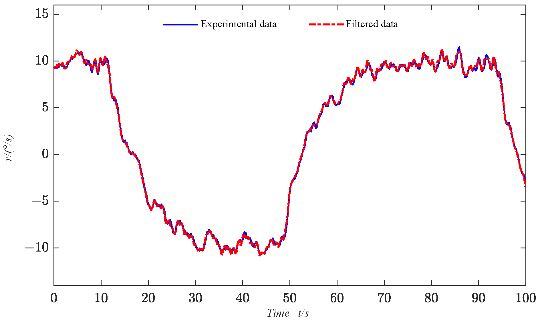
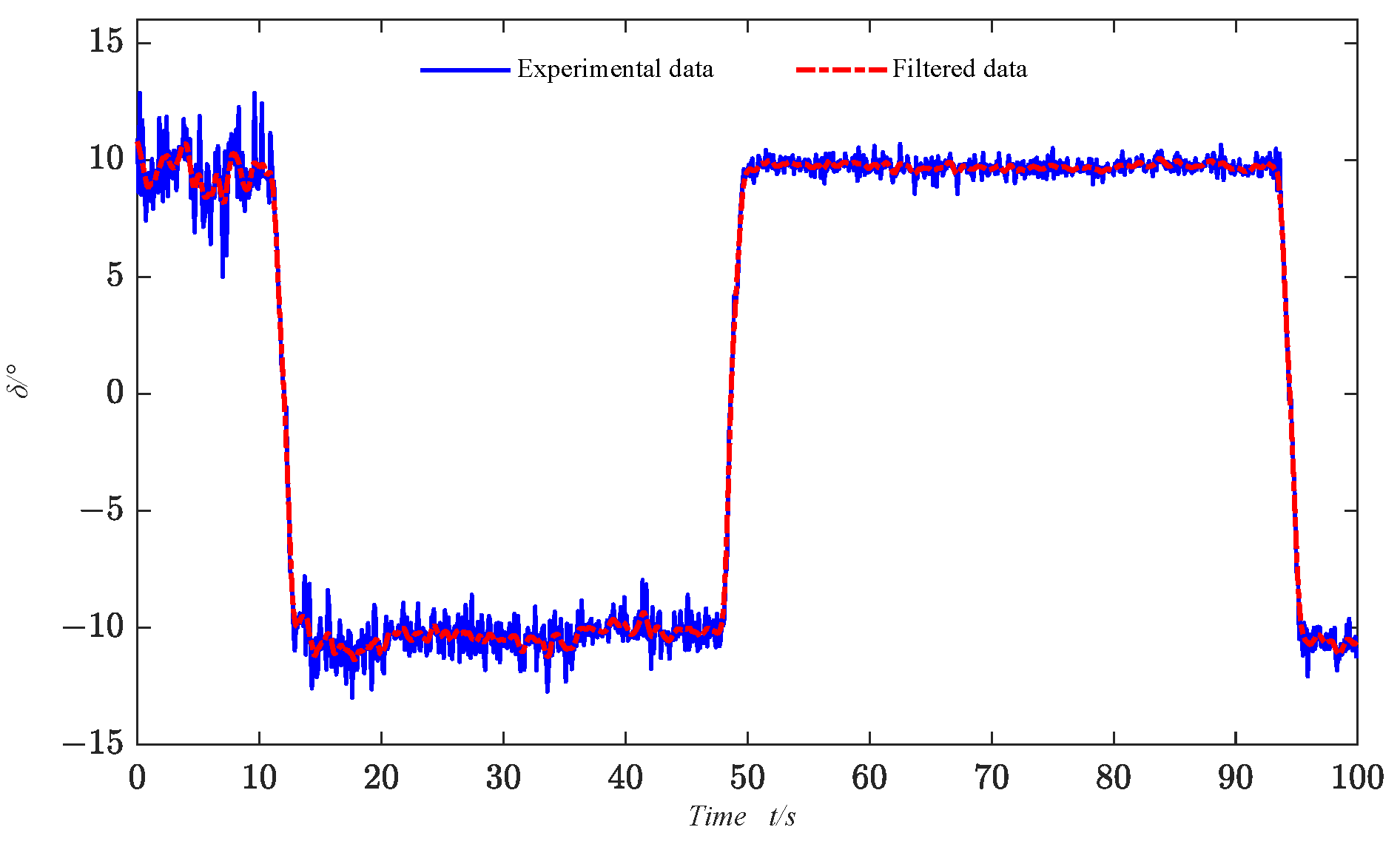
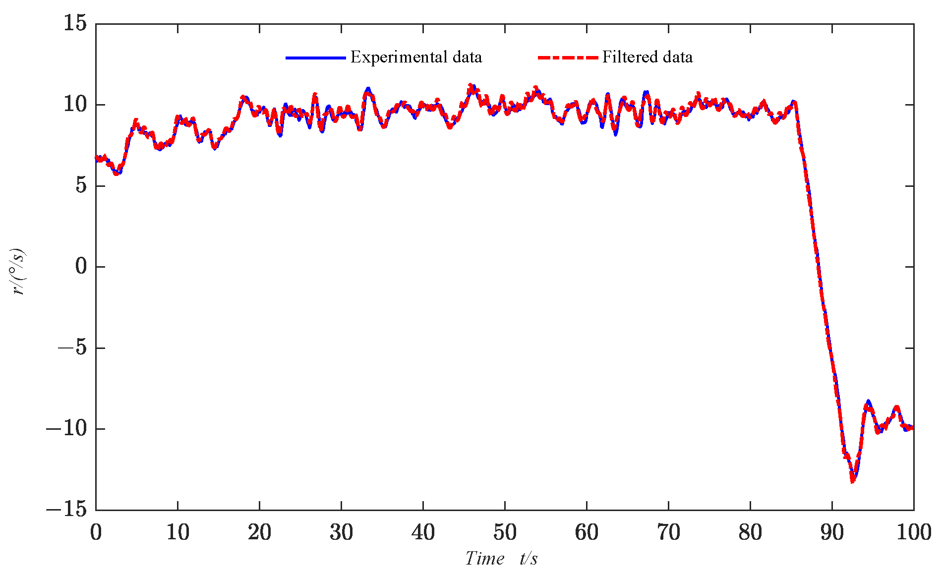
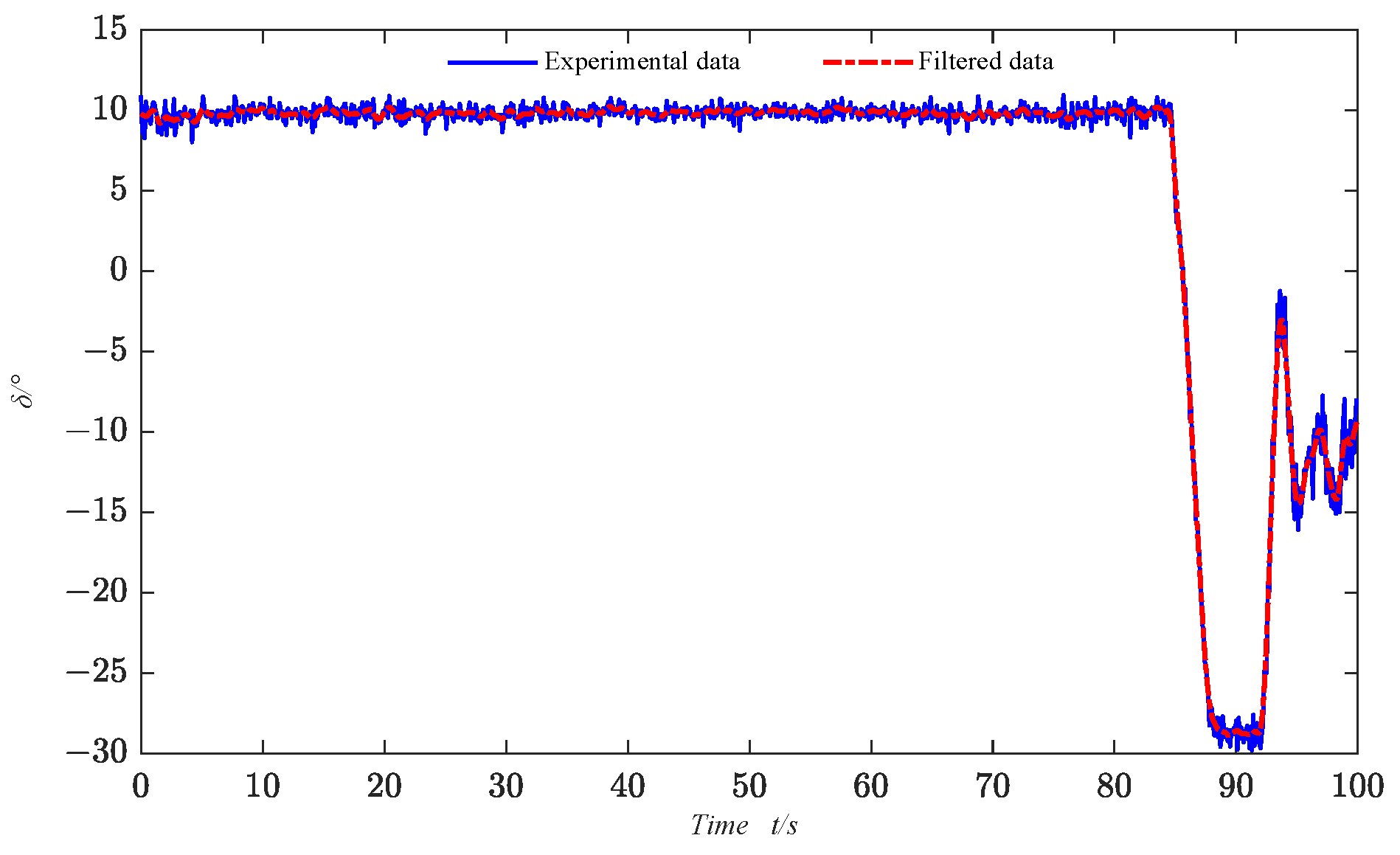
Various environmental and external uncertainties interfere with the USV’s motion during navigation, and there may be mutual influences between sensors. As a result, the collected motion state data often contain various disturbances. To improve the parameter identification results and obtain a more accurate USV maneuvering model, the sensor data are filtered. In this paper, the LWR filtering algorithm is employed to process the data.

Assuming the number of sampled data is denoted as $m_1$ and the total number of data is $l$, to facilitate the selection of the fitting position, $m_1$ is chosen as an odd number. The equation at the fitting position is then defined as:

$$G\left(x\right)={\beta }_1\left(x\right)+{\beta }_2\left(x\right)x+{\beta }_3\left(x\right)x^2+\epsilon$$

(6)

where $x$ is the time coordinate at the fitting point within the data window, and $\epsilon$ represents the random fitting error. $\mathit{\beta }\left(x\right)=[{\beta }_1(x),{\beta }_2(x),{\beta }_3(x)]$ is the parameter vector of the equation at the fitting point.

To obtain the parameter vector, weighted regression is performed on the data within the data window. In the actual filtering process, the weight at each position within the data window is determined by its distance from the fitting point. Typically, the farther the position is from the fitting point, the smaller the weight. Therefore, a cubic weighting function is used to determine the weights:

$$\left\{\begin{array}{l}W\left(k\right)={\left(1-d^3\left(k\right)\right)}^3\\ d\left(k\right)=2\left|x\left(k\right)-x\right|/(m_1-1)\end{array}\right.$$

(7)

where $x\left(k\right), \mathrm{k}=1,2,\dots ,m_1$ are time coordinates of each point within the data window.

After obtaining the weights for each position using Equation (7), a WLS algorithm is designed to estimate the coefficients in Equation (6). The following three matrices are defined based on the experimental data:

$$\left\{\begin{array}{l}\mathit{A}=\left[\begin{array}{ccc}1& x\left(1\right)& x^2\left(1\right)\\ 1& x\left(2\right)& x^2\left(2\right)\\ ⋮& ⋮& ⋮\\ 1& x\left(m_1\right)& x^2\left(m_1\right)\end{array}\right]\\ \mathit{B}={\left[\begin{array}{cccc}G\left(1\right)& G\left(2\right)& \cdots & G\left(m_1\right)\end{array}\right]}^T\\ \mathit{C}=diag\left[W\left(1\right)W\left(2\right) ··· W\left(m_1\right)\right]\end{array}\right.$$

(8)

According to Equations (6) and (8), the objective function for parameter $\mathit{\beta }\left(x\right)$ can be expressed as:

$$\min J\left(\beta \right)={\left[\mathit{B}-\mathit{A}\mathit{\beta }(x)\right]}^T·\mathit{C}·\left[\mathit{B}-\mathit{A}\mathit{\beta }(x)\right]$$

(9)

Based on the fundamental principle of the LS method, the solution formula for parameter $\mathit{\beta }\left(x\right)$ can be expressed as:

$$\beta \left(x\right)={\left({\mathit{A}}^T\varphi \mathit{A}\right)}^{-1}{\mathit{A}}^T\varphi \mathit{B}$$

(10)

According to Equation (10), the coefficients in Equation (6) can be obtained, which in turn leads to the complete filtering equation that allows the filtering of the USV motion data required for identification as described in Equation (6).

3. The Design of the EKF Algorithm

Assuming that the state equation of a discrete nonlinear system is given as follows:

$$\left\{\begin{array}{l}{\mathit{X}}_{k+1}=f({\mathit{X}}_k,{\mathit{W}}_k,k)\\ {\mathit{Z}}_k=c({\mathit{X}}_k,{\mathit{V}}_k,k)\end{array}\right.$$

(11)

where $\mathit{X}$ is the state vector; $f(•)$ is the n-dimensional nonlinear state vector transfer function; $\mathit{Z}$ is the output vector; $c(•)$ is the m-dimensional nonlinear vector-valued function; $\mathit{W}$ and $\mathit{V}$ are the system process noise and measurement noise, respectively, both being Gaussian white noises with zero mean.

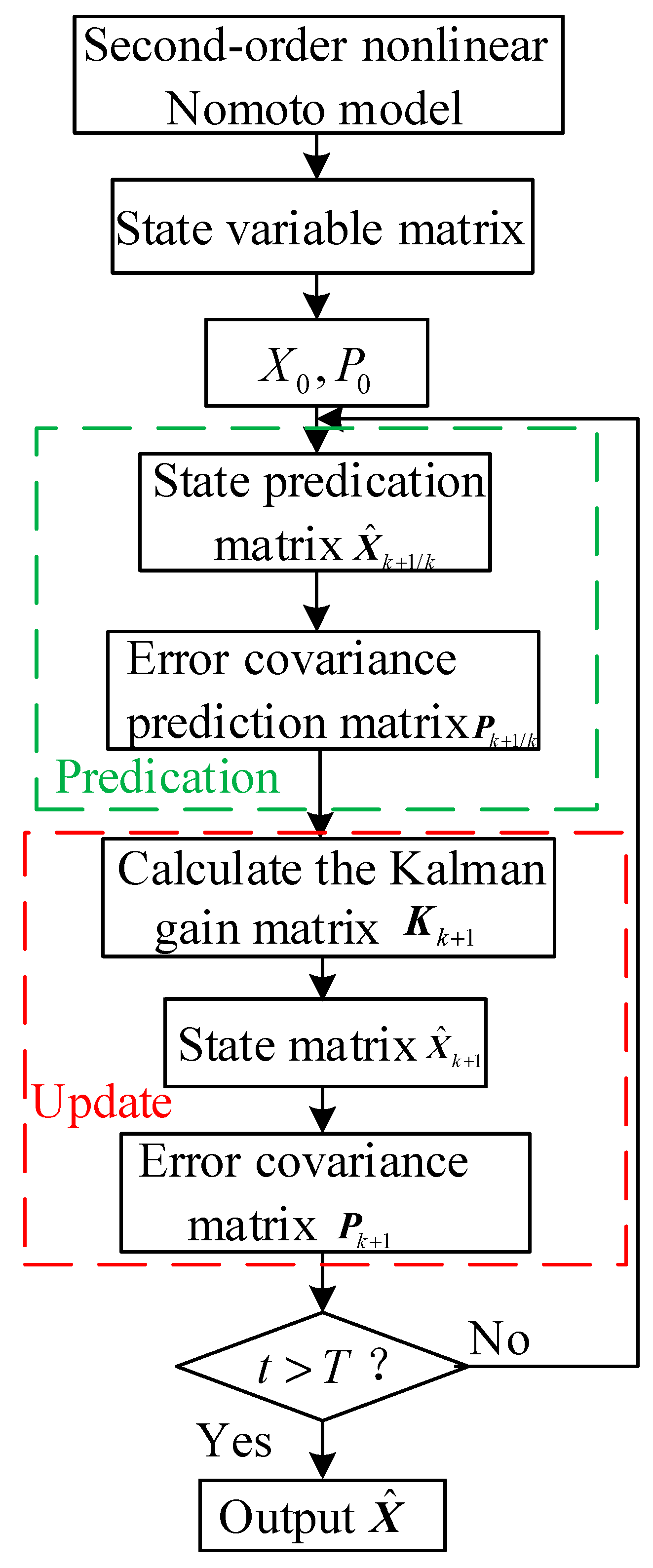
The recursive process for the parameter estimation of the system based on the EKF algorithm is shown in the following Figure 1:

When parameter identification is performed based on the EKF algorithm, the parameters to be identified need to be included in the state vector, and the identification parameters are obtained through the overall estimation of the state variables. The EKF algorithm is mainly divided into prediction and update phases, with the specific calculation formulas for each stage shown as follows:

(1) The prediction phase includes the calculation of the state matrix ${\widehat{\mathit{X}}}_{k+1/k}$ and the error covariance matrix ${\mathit{P}}_{k+1/k}$:

$$\left\{\begin{array}{l}{\widehat{\mathit{X}}}_{k+1}=f({\mathit{X}}_k,k)\\ {\mathit{P}}_{k+1/k}={\mathit{\Phi }}_{k+1/k}{\mathit{P}}_k{\mathit{\Phi }}_{k+1/k}^T+{\mathit{Q}}_{k+1}\end{array}\right.$$

(12)

(2) The update phase includes the calculation of the Kalman gain matrix ${\mathit{K}}_{k+1}$, as well as the update of the state matrix ${\widehat{\mathit{X}}}_{k+1}$ and the error covariance matrix ${\mathit{P}}_{k+1}$:

$$\left\{\begin{array}{l}{\mathit{K}}_{k+1}={\mathit{P}}_{k+1/k}{\mathit{L}}_{k+1}^T{({\mathit{L}}_{k+1}{\mathit{P}}_{k+1/k}{\mathit{L}}_{k+1}^T+{\mathit{R}}_{k+1})}^{-1}\\ {\widehat{\mathit{X}}}_{k+1}={\widehat{\mathit{X}}}_{k+1/k}+{\mathit{K}}_{k+1}[{\mathit{Z}}_k-c({\widehat{\mathit{X}}}_{k+1/k})]\\ {\mathit{P}}_{k+1}={\mathit{P}}_{k+1/k}-{\mathsf{K}}_{k+1}{\mathsf{L}}_{k+1}{\mathsf{P}}_{k+1/k}\end{array}\right.$$

(13)

In the above process, both the state equation and the measurement equation are utilized. The EKF algorithm performs measurement updates based on the measurement equation, allowing the measurement data to correct the state error and achieve higher estimation accuracy.

When designing the state vector, the parameters $\mathit{\theta }$ and $\mathit{Y}$ to be identified in Equation (4) need to be combined into a new system state variable ${\mathit{X}}_{\mathit{k}}$:

$${\mathit{X}}_{\mathit{k}}={\left[x_1 x_2 x_3 x_4 x_5 x_6 x_7\right]}^T$$

(14)

where $x$ can be written as follows:

$$\left\{\begin{array}{l}{x}_1=Y\\ x_i=\theta (i-1) , i=2,3,···,7\end{array}\right.$$

(15)

The state transition matrix of the system can be expressed as:

$${\mathit{\Phi }}_{k+1/k}=\left[\begin{array}{cccc}0& H(1)& \cdots & H(6)\\ 0& 1& \cdots & 0\\ 0& 0& \cdots & 0\\ ⋮& ⋮& \ddots & ⋮\\ 0& 0& 0& 1\end{array}\right]$$

(16)

The system state equation can be obtained from Equations (14) and (16) as follows:

$${\mathit{X}}_{k+1}={\mathit{\Phi }}_{k+1/k}{\mathit{X}}_k$$

(17)

Assuming the observation matrix can be written as follows:

$${\mathit{L}}_{k+1}=\left[1 0 0 0 0 0 0\right]$$

(18)

Combining Equations (17) and (18), the observation matrix can be obtained as follows:

$${\mathit{Z}}_{k+1}={\mathit{L}}_{k+1}{\mathit{X}}_{k+1}$$

(19)

After constructing the state equation and observation equation, the parameters in the second-order nonlinear Nomoto model can be identified through the EKF algorithm process.

4. Identification Results and Analysis

4.1. Overview of the Full-Scale Vessel

Parameter identification research is conducted in this paper based on full-scale experimental data from a USV, with the main parameters of the USV shown in

Table 1. Main parameters of USV.

Parameter	Value	Parameter	Value
Length/m	11.0	Width/m	3.20
Draught/m	0.63	Mass/kg	8000.0

:

In this paper, a real-ship experiment was conducted using a full-scale USV in the offshore waters near Sanya, Hainan Province, under two different operational conditions. The specific experimental steps are as follows:

(1) Operational Condition 1: 10°/−10° Steering Experiment: The USV was operated at its rated speed with a steering angle of 10° for 50 s, followed by a steering angle of −10° for the same duration. To minimize the impact of random occurrences, the experiment was repeated 4 times. The experimental data obtained were primarily used for the identification modeling of the USV’s maneuverability parameters and to verify the accuracy of the resulting model.

(2) Operational Condition 2: 10°/−10° Turning Experiment: The USV was operated at its rated speed with a steering angle of 10° or −10° for a duration of 50 s.

In this study, the motion data required for identification include the yaw rate, yaw angle, and steering angle. The yaw angle is measured by an inertial navigation sensor, while the steering angle is obtained from the control-end sensor. To more effectively handle nonlinear data and the dynamic performance of varying systems, we applied filtering to the experimental data collected from the sensors. The yaw rate is derived by differentiating the filtered yaw angle.

4.2. Full-Scale Vessel Data and Filtering Processing Results

The USV motion data required for identification include the rudder angle $\delta$ and the heading rate $r$. Two sets of 100-s motion data under different operating conditions are selected for the parameter identification of the USV Nomoto model. The hardware platform is a 2.59 GHz CPU and has 8 GB memory, and the software platform is OCTAVE 9.3.0. The results of the filtering of the real vessel data using LWR are shown in Figure 2, Figure 3, Figure 4 and Figure 5:

4.3. Identification Result

In order to verify the identification performance of the EKF algorithm mentioned above, parameter identification of the second-order nonlinear Nomoto model is performed based on the filtered real vessel data. The initial values are set as follows:

$$\left\{\begin{array}{l}{\mathit{X}}_0={[0.01 0.01 0.01 0.01 0.01 0.01 0.01]}^T\\ P_0={10}^6\times I_7\end{array}\right.$$

(20)

The obtained identification results are shown in

Table 2. EKF parameter identification results.

Parameter	Value	Parameter	Value
$K$	0.5770	$T_1$	2.5384
${\delta }_r$	0.0137	$T_2$	0.7097
$a$	61.7745	$T_3$	0.9460

below:

4.4. Simulation Verification

In order to verify the accuracy of the parameter identification values obtained by the EKF algorithm, the identified parameters are substituted into the second-order nonlinear Nomoto model. The same rudder angle as the real vessel data is used as the input, and the simulated heading angle and heading rate data are obtained for comparison. The results are shown in Figure 6, Figure 7, Figure 8, Figure 9, Figure 10, Figure 11, Figure 12 and Figure 13:

From the heading angle forecast results (Figure 6 and Figure 10) and the heading rate forecast results (Figure 8 and Figure 12), it can be visually observed that, under both operating conditions, the predicted curves for heading angle and heading rate closely match the experimental data. As shown in Figure 7 and Figure 11, the prediction errors for the heading angle remain within 18°, and in Figure 9 and Figure 13, the prediction errors for the heading rate stay within 8°/s. This demonstrates that the parameters identified by the EKF algorithm are highly accurate, with excellent modeling precision.

To more clearly demonstrate the accuracy of the identification and modeling performed by the EKF algorithm, the MAE and the R² are introduced as evaluation metrics for algorithm precision [23]. The calculation formulas are given as follows:

$$\left\{\begin{array}{l}\mathrm{MAE}={\displaystyle \sum _{i=1}^n\left|y_i-{\widehat{y}}_i\right|/n}\\ {\mathrm{R}}^2=1-[{\displaystyle \sum _{i=1}^n{\left(y_i-{\widehat{y}}_i\right)}^2}/{\displaystyle \sum _{i=1}^n{\left(y_i-\overline{y}\right)}^2]}\end{array}\right.$$

(21)

where $y_i$ represents the real vessel data; ${\widehat{y}}_i$ represents the simulated prediction values; $n$ denotes the number of data points; and $\overline{y}$ represents the mean of the measurement values.

MAE can measure the average error between the predicted data and the experimental data, while R² can be used to evaluate the fitting performance of the identified model. The closer R² is to 1, the higher the algorithm’s accuracy. The MAE and R² values calculated under the two operating conditions are shown in

Table 3. MAE and R² values calculation results (Case 1).

	$\mathit{\psi }$		$\mathit{r}$
Value	RLS	EKF	RLS	EKF
MAE	31.71	4.908	1.916	1.342
R2	0.864	0.996	0.868	0.945

and

Table 4. MAE and R² values calculation results (Case 2).

	$\mathit{\psi }$		$\mathit{r}$
Value	RLS	EKF	RLS	EKF
MAE	12.5625	9.8472	0.688	0.630
R2	0.9972	0.9981	0.962	0.974

and Figure 14 and Figure 15:

It can be seen from Table 3 and Table 4 that the forecast heading angle MAE indicator for both conditions using the EKF algorithm is within 10°, the forecast heading rate MAE indicator is within 1.5°/s, and the R² values for the forecast heading angle and heading rate are both above 0.94. In contrast, as shown in Figure 14 and Figure 15, the RLS algorithm results in forecast heading angle MAE indicators exceeding 10° for both conditions, the forecast heading rate MAE indicator is close to 2°, and the R² values for the forecast heading angle and heading rate are around 0.86. Compared to the RLS algorithm, the heading angle MAE values are improved by 93.95% and 21.61%, respectively, with the EKF-based approach, while the heading rate values are improved by 72.65% and 8.43%, respectively. This demonstrates that the performance of the EKF algorithm is significantly superior to that of the RLS algorithm, and the second-order nonlinear Nomoto model identified and established using the EKF algorithm closely matches the actual heading response state of the USV.

4.5. Model Generalization Ability Analysis

In order to test the generalization ability of the model, real-ship data from another set of conditions (5° turning experiment) were used for the parameter identification and modeling study of the USV. The simulation results are shown in Figure 16, Figure 17, Figure 18 and Figure 19:

The calculated MAE and R² values are shown in

Table 5. MAE and R² values calculation results (Case 3).

	$\mathit{\psi }$		$\mathit{r}$
Value	RLS	EKF	RLS	EKF
MAE	9.8304	9.3364	0.7595	0.7369
R2	0.920	0.935	0.970	0.974

and Figure 20:

As can be seen from Figure 16 and Figure 18, the forecasted curves of the heading angle and heading rate are well fitted. And it can be observed from Figure 15 and Figure 17 that the prediction error of the EKF is smaller than that of the RLS. From the calculation results in Table 5, it can be observed that the MAE indicator of the forecasted heading angle is within 9.5°, the MAE indicator of the forecasted heading rate is within 0.74°/s, and the R² values of the forecasted heading angle and heading rate are both above 0.93. However, the MAE indicator of the forecasted heading angle is over 9.8°, the MAE indicator of the forecasted heading rate is over 0.75°, and the R² values of the forecasted heading angle are below 0.93, as shown in Figure 20. Compared to the RLS algorithm, the heading angle MAE values are improved by 5.03% with the EKF-based approach, while the heading rate values are improved by 3.0%. These results demonstrate that the EKF algorithm outperforms the RLS algorithm, as the USV Nomoto model established using the EKF algorithm achieves higher accuracy in forecasting both the heading angle and heading rate. Furthermore, the EKF algorithm exhibits strong generalization ability.

To further help understand the robustness of the model, this paper sets the bow angle error to 17° and the bow angular velocity error to 2°/s as confidence intervals. The counts exceeding the confidence interval for two methods in the 10°/−10° turning experiment (Case 1), 10°/−10° turning experiment (Case 2), and 5° turning experiment were compiled, and the results are shown in the following table.

According to

Table 6. The number of values outside the confidence interval.

Case	Case 1		Case 2		Case 3
Values	${\mathit{\psi }}_{\mathit{e}}$	${\mathit{r}}_{\mathit{e}}$	${\mathit{\psi }}_{\mathit{e}}$	${\mathit{r}}_{\mathit{e}}$	${\mathit{\psi }}_{\mathit{e}}$	${\mathit{r}}_{\mathit{e}}$
EKF	11	262	0	62	134	26
RLS	479	307	125	75	173	59

, the number of bow angle errors and bow angular velocity errors exceeding the confidence interval of the EKF algorithm under three different operating conditions is significantly lower than that of the RLS algorithm. This further indicates that the EKF algorithm has stronger robustness and accuracy compared to the RLS algorithm.

4.6. Sensitivity Analysis of Hydrodynamic Coefficients Based on the Indirect Method

Sensitivity analysis is essential because it helps identify which parameters have the greatest impact on the results, thus providing important insights for optimization and decision-making. The sensitivity of the hydrodynamic coefficients to each motion state variable is defined as follows:

$$\left\{\begin{array}{l}{S}^{\psi }=[\max (|{\tilde{\psi }}^{\prime }\left(t\right)-{\psi }^{\prime }\left(t\right)|)]/SUM\\ S^r=[\max (|{\tilde{r}}^{\prime }\left(t\right)-r^{\prime }\left(t\right)|)]/SUM\\ SUM=\left([\max (|{\tilde{\psi }}^{\prime }\left(t\right)-{\psi }^{\prime }\left(t\right)|)]+[\max (|{\tilde{r}}^{\prime }\left(t\right)-r^{\prime }\left(t\right)|)]\right)\end{array}\right.$$

(22)

This method applies a specific percentage perturbation to a particular hydrodynamic coefficient and then performs a maneuvering motion numerical simulation. The change in motion state variables from the simulation results is used as the basis for calculating the sensitivity value. In this paper, a 1.1 times perturbation is applied to six parameters to observe their sensitivity, and the $S^{\psi }$ data are as follows (

Table 7. Sensitivity analysis of hydrodynamic coefficients.

Parameters	$\mathit{K}$	${\mathit{T}}_1$	${\mathit{T}}_2$	${\mathit{T}}_3$	$\mathit{\alpha }$	${\mathit{\sigma }}_{\mathit{r}}$
Original value (Case 1)	0.6660	0.6660	0.6660	0.6660	0.6660	0.6660
Perturbed value (Case 1)	0.6628	0.6681	0.6659	0.6660	0.6659	0.6662
Original value (Case 2)	0.9737	0.9737	0.9737	0.9737	0.9737	0.9737
Perturbed value (Case 2)	0.9752	0.9739	0.9736	0.9736	0.9670	0.9737
Original value (Case 3)	0.9883	0.9883	0.9883	0.9883	0.9883	0.9883
Perturbed value (Case 3)	0.9899	0.9884	0.9883	0.9881	0.9873	0.9880

):

From Table 7, it can be seen that after increasing the six parameters identified by 1.1 times under three operating conditions, the effect of changing parameter $K$ on the sensitivity parameters $S^{\psi }$ is the greatest, followed by $\alpha$ and ${\sigma }_r$, while $T_1,T_2,T_3$ have a smaller sensitivity on the model.

5. Conclusions

A motion mathematical model for the USV second-order nonlinear Nomoto model was established in this paper, and the parameters in the model were identified using the EKF algorithm combined with real-ship data. The LWR algorithm was applied to smooth and filter the collected sensor data, and the EKF algorithm was used to identify the parameters of the USV second-order nonlinear Nomoto model. The forecast of the USV trajectory demonstrated that the EKF algorithm achieves very high identification accuracy, and the established model meets the requirements for USV maneuverability prediction. Future research will focus on extending the model to account for more complex operational environments and investigating real-time data assimilation strategies to improve operational efficiency. These efforts aim to advance the practical application of the Nomoto model in various maritime scenarios.

References

1. Zhang, X.G.; Zou, Z.J. Identification of Abkowitz model for ship manoeuvring motion using ε-support vector regression. J. Hydrodyn. 2011, 23, 353–360. [Google Scholar] [CrossRef]
2. Dong, Z.P.; Zhou, W.J.; Tan, F.; Wang, B.L.; Wen, Z.Y.; Liu, Y.C. Simultaneous modeling and adaptive fuzzy sliding mode control scheme for underactuated USV formation based on real-time sailing state data. Ocean Eng. 2024, 314, 119743. [Google Scholar] [CrossRef]
3. Li, W.; Zhang, J.; Wang, F.; Zhou, H.Y. Model predictive control based on state space and rise augmentation for unmanned surface vessel trajectory tracking. J. Mar. Sci. Eng. 2023, 11, 2283. [Google Scholar] [CrossRef]
4. Clarke, D.P.; Gedling, P.; Hine, G. The application of manoeuvring criteria in hull design using linear theory. Nav. Archit. 1983, 125, 45–68. [Google Scholar]
5. Song, J.L.; Cheney, J.A.; Bomphrey, R.J.; Usherwood, J.R. Virtual manipulation of tail postures of a gliding barn owl (Tyto alba) demonstrates drag minimization when gliding. J. R. Soc. Interface 2022, 19, 20210710. [Google Scholar] [CrossRef]
6. Dong, Z.P.; Wang, B.L.; Tan, F.; Zhou, W.J.; Liu, Y.C. Online parameter identification and real-time manoeuvring prediction for a water-jet USV based on weighted multi-innovation prediction error method integrated with dynamic window strategy. Appl. Ocean Res. 2024, 153, 104260. [Google Scholar] [CrossRef]
7. Sayed, P.T.; Simon, J.; Danilo, P. Filtering structures for α-stable systems. IEEE Control Syst. Lett. 2022, 7, 553–558. [Google Scholar]
8. Dong, Z.P.; Yang, X.; Zheng, M.; Song, L.F.; Mao, Y.S. Parameter identification of unmanned marine vehicle manoeuvring model based on extended Kalman filter and support vector machine. Int. J. Adv. Robot. Syst. 2019, 16, 1729881418825095. [Google Scholar] [CrossRef]
9. Zhao, B.G.; Zhang, X.K.; Liang, C.L. A novel parameter identification algorithm for 3-DOF ship maneuvering modelling using nonlinear multi-innovation. J. Mar. Sci. Eng. 2022, 10, 581. [Google Scholar] [CrossRef]
10. Ouyang, Z.L.; Zou, Z.J. Nonparametric modeling of ship maneuvering motion based on Gaussian process regression optimized by genetic algorithm. Ocean Eng. 2021, 238, 109699. [Google Scholar] [CrossRef]
11. Yin, Y.; He, Q.; Hu, F.M.; Huang, W.F. Merging experiment data and simulation data for parameter identification of shaft seal. Measurement 2024, 236, 114863. [Google Scholar] [CrossRef]
12. Li, S.Y.; Wang, T.T.; Li, G.Y.; Zhang, H.X. Ship maneuvering model optimization for improved identification with less excitation. Ocean Eng. 2023, 280, 114540. [Google Scholar] [CrossRef]
13. Wu, J.B.; Zeng, C.H.; Hu, Y.F. Indirect adaptive robust control design for course tracking of ships subject to unknown control coefficient and disturbances. Int. J. Control. Autom. Syst. 2021, 19, 2059–2067. [Google Scholar] [CrossRef]
14. Meng, Y.; Zhang, X.K.; Zhang, X.F.; Duan, Y.T. Maneuverability indices estimation of nonlinear response model based on full-scale trial data and square root unscented Kalman filter. Ocean Eng. 2023, 286, 115699. [Google Scholar] [CrossRef]
15. Xu, L.; Ding, F.; Zhang, X.; Zhu, Q.M. Novel parameter estimation method for the systems with colored noises by using the filtering identification idea. Syst. Control Lett. 2024, 186, 105774. [Google Scholar] [CrossRef]
16. Xin, D.J.; Shi, L.F. Kalman filter for linear systems with unknown structural parameters. IEEE Trans. Cricuits Syst. II Express Briefs. 2022, 69, 1852–1856. [Google Scholar] [CrossRef]
17. Saha, J.; Bhaumik, S. Robust maximum correntropy Kalman filter. Int. J. Robust Nonlinear Control. 2024. [Google Scholar] [CrossRef]
18. Lou, T.S.; Chen, N.H.; Zhao, L.Y. Adaptive fast desensitized Kalman filter. Circuits Syst. Signal Process. 2024, 43, 7364–7386. [Google Scholar] [CrossRef]
19. Lin, D.Y.; Zhang, Q.Q.; Chen, X.F.; Wang, S.Y. Maximum correntropy quaternion Kalman filter. IEEE Trans. Signal Process. 2023, 71, 2792–2803. [Google Scholar] [CrossRef]
20. Mosconi, L.; Farroni, F.; Sakhnevych, A.; Timpone, F.; Gerbino, F.S. Adaptive vehicle dynamics state estimator for onboard automotive applications and performance analysis. Veh. Syst. Dyn. 2023, 61, 3244–3268. [Google Scholar] [CrossRef]
21. Feng, S.; Li, X.G.; Zhang, S.; Jian, Z.; Duan, H.X.; Wang, Z.P. A review: State estimation based on hybrid models of Kalman filter and neural network. Syst. Sci. Control Eng. 2023, 11, 2173682. [Google Scholar] [CrossRef]
22. Zhong, Y.M.; Yu, C.Y.; Wang, R.; Pei, T.Q.; Lian, L. Adaptive anti-noise least-squares algorithm for parameter identification of unmanned marine vehicles: Theory, simulation, and experiment. Int. J. Fuzzy Syst. 2023, 25, 369–381. [Google Scholar] [CrossRef]
23. Uyanik, T.; Yalman, Y.; Kalenderli, O.; Arslanoglu, Y.; Terriche, Y.; Su, C.L.; Guerrero, J.M. Data-driven approach for estimating power and fuel consumption of ship: A case of container vessel. Mathematics 2022, 10, 4167. [Google Scholar] [CrossRef]
Figure 1. Schematic diagram of the EKF algorithm.
Applsci 15 00161 g001
Figure 2. Filtering effect of heading angular velocity data (Case 1).
Applsci 15 00161 g002
Figure 3. Filtering effect of rudder angle data (Case 1).
Applsci 15 00161 g003
Figure 4. Filtering effect of heading angular velocity data (Case 2).
Applsci 15 00161 g004
Figure 5. Filtering effect of rudder angle data (Case 2).
Applsci 15 00161 g005
Figure 6. Prediction results of heading angle (Case 1).
Applsci 15 00161 g006
Figure 7. Prediction errors of heading angle (Case 1).
Applsci 15 00161 g007
Figure 8. Prediction results of heading angular velocity (Case 1).
Applsci 15 00161 g008
Figure 9. Prediction errors of heading angular velocity (Case 1).
Applsci 15 00161 g009
Figure 10. Prediction results of heading angle (Case 2).
Applsci 15 00161 g010
Figure 11. Prediction errors of heading angle (Case 2).
Applsci 15 00161 g011
Figure 12. Prediction results of heading angular velocity (Case 2).
Applsci 15 00161 g012
Figure 13. Prediction errors of heading angular velocity (Case 2).
Applsci 15 00161 g013
Figure 14. Calculation results (Case 1). (a) with MAE; (b) with R2.
Applsci 15 00161 g014
Figure 15. Calculation results (Case 2). (a) with MAE; (b) with R2.
Applsci 15 00161 g015
Figure 16. Prediction results of heading angle (Case 3).
Applsci 15 00161 g016
Figure 17. Prediction errors of heading angle (Case 3).
Applsci 15 00161 g017
Figure 18. Prediction results of heading angular velocity (Case 3).
Applsci 15 00161 g018
Figure 19. Prediction errors of heading angular velocity (Case 3).
Applsci 15 00161 g019
Figure 20. Calculation results (Case 3). (a) with MAE; (b) with R2.
Applsci 15 00161 g020