Featured Application
Inspection of structures, e.g., offshore/nuclear/eolic plants, bridges, and tall buildings. Inspection of archaeological sites. Placement and retrieval of sensors. Assembly of structures in places not accessible/safe for humans.
Abstract
The precise control of an aerial manipulator presents a formidable challenge due to the inherent mobility of its base, which is subject to both external disturbances and dynamic disturbances due to manipulator motions. In this paper, we introduce two Closed-Loop Inverse Kinematics (CLIK) control algorithms tailored to aerial manipulators. The first algorithm operates at the velocity level and uses the Generalized Jacobian for inverse kinematics, while the second one operates at the acceleration level. We evaluate their performance in a simulated environment, replicating real-world challenges such as the wind effect, sensors noise, uncertainty of the system inertial parameters, and impulsive forces at the end-effector. Trajectory tracking simulated experiments are carried out for a two- and three-degree-of-freedom (DOF) aerial manipulator tracking a circular trajectory with its end-effector. Both algorithms demonstrate promising results in coping with external disturbances and variations in the inertial parameters, enhancing the precision of the trajectory tracking control. The acceleration-level algorithm shows overall better performance compared to the velocity-level one in the face of greater implementation complexity and computational burden.
1. Introduction
In recent years, a notable interest in the adoption of autonomous systems, such as aerial manipulators, has grown. They can be used for the execution of safety-critical and resource-intensive tasks within various industrial domains. These applications encompass a wide range of activities, including the inspection, assembly, and maintenance of mechanical structures, as well as general inspection and maintenance duties where the enhanced maneuverability of aerial manipulators can be exploited [1,2].
An Unmanned Aerial Manipulator (UAM) consists of a robotic manipulator attached to an Unmanned Aerial Vehicle (UAV). Multicopters with multiple rotors, which are capable of stable hovering, are the most common choice for the base configuration, ensuring stability while the manipulator executes its tasks [3]. Various designs have been considered for the robotic manipulator, from task-specific grippers to hyper-redundant arms [1,3], lightweight manipulators [4], and additional arms to stabilize the UAV [5].
The coupling of kinematics and dynamics between UAV and manipulator presents a particular challenge in achieving the precise positioning and control of the end-effector, especially for complex tasks like grasping, due to the motion of the UAV during the maneuver. Two main strategies exist for the control of a UAM: in the coupled strategy, the dynamics of the whole system is considered [6], while in the decoupled strategy, the manipulator and the UAV have distinct control systems [1].
Certain approaches aim to reduce the base motion at the mechanical design level, employing counter-balancing mechanisms or mass distribution strategies [7], while other methods exploit the kinematic redundancy of the manipulator to minimize the dynamic disturbance transferred from the manipulator to the UAV [8,9]. On the other hand, in space robotics, the control of floating-base manipulators has been addressed assuming the conservation of momentum [10] to compensate for base motions. In this field, inverse kinematic control algorithms based on the Generalized Jacobian enable the precise positioning of the end-effector. An adaptation of the Generalized Jacobian for aerial manipulation is detailed in [9], where gravity and UAV control forces are also considered.
CLIK (Closed-Loop Inverse Kinematics) [11] strategies have already been applied to aerial manipulation. In [12], a first-order CLIK algorithm fed by an impedance control module generates reference values for joint angles, UAV position, and its attitude. In [13], a second-order CLIK algorithm working on joint angles, UAV position, and attitude is used. A first-order CLIK algorithm with integral action is introduced in [14]. In [15], the CLIK algorithm with the adjoint of an integral action is used to control the robotic arm, and the UAV is controlled by a distinct non-linear controller; the UAV controller also generates a reference for the torque between the UAV and the robotic arm, and then this torque demand is fulfilled as a secondary task in the CLIK algorithm.
In this paper, we propose two novel methods for the solution of the inverse kinematics of serial aerial manipulators to perform trajectory tracking tasks. Both methods are derived from CLIK schemes for fixed-base manipulators and are adapted to take into account UAV motion. These algorithms are used to compute the joint trajectories corresponding to the desired end-effector trajectory; these then constitute the reference input for some feedback kinematic control scheme at the level of joint velocities or accelerations that ensures the desired precision even in the presence of modeling uncertainties and/or unknown disturbances.
The proposed methods for the solution of the inverse kinematics consider and compensate for UAV motions caused by the reaction forces/torques due to the robotic arm motion and by known forces/torques (gravity, control forces and torques). At the same time, the feedback of CLIK algorithms is used to compensate for modeling errors and other disturbances. The combination of these two techniques is a novel contribution to the field of aerial manipulation.
The first algorithm operates at the velocity level and is based on the Generalized Jacobian method adapted to aerial manipulators [9]. As for CLIK algorithms, they include a feedback term on the joint velocities to compensate for the position error of the end-effector due to unknown disturbances and modeling errors. Then, we implement an acceleration-level algorithm with feedback on the joint accelerations to control the aerial manipulator. The two proposed methods are implemented and validated in MATLAB (release 2023b) for a UAM subject to the following disturbances: unpredicted aerodynamic forces, noise in sensors measurement, and errors between the inertial parameters of the system used in the solution of the inverse kinematics and the real UAM ones. We also test the system response to impulsive disturbance forces at the end-effector.
The UAV and aerial manipulator dynamics are presented in Section 2. The two CLIK algorithms for aerial manipulators are introduced in Section 3: the first-order algorithm with feedback on the joint velocities of the robotic arm and the second-order algorithm with feedback on the joint accelerations. The simulation setup for the validation of the proposed methods and the models for disturbances and measurements noise are presented in Section 4. Section 5 reports the simulation results, which demonstrate the trajectory tracking and disturbance rejection capabilities of our methods.
2. System Modeling
Our system is an octocopter drone with a planar serial robotic arm mounted beneath it. The UAV base and the arm are modeled as two distinct but dynamically coupled systems, i.e., the motion of each of the two systems affects the other because of the reaction forces and torques they exchange at their mechanical interface. These two systems are controlled separately: (1) the UAV is controlled through a Proportional–Integral–Derivative (PID) algorithm to maintain its hovering state, while (2) the arm is controlled through a CLIK algorithm that also takes into account the base movements.
In the following subsections, first, the dynamic model of the base and its control are presented, and then the kinematics and dynamics of the flying-base manipulators are derived. These models are the foundation of the control algorithms described in Section 3.
2.1. UAV Base Dynamics and Control
The UAV is modeled as a rigid body of mass with a moment of inertia around its barycenter of . Its parameters are based on those of the commercial octocopter S1000 Spreading Wings manufactured by DJI (Shenzhen, China).
In the discussion of the system dynamic model, the following reference frames are used: the fixed inertial reference frame, denoted by the subscript , and the body-fixed reference frame, denoted by the subscript , whose origin is positioned on the base Center of Gravity (CoG). The vertical axis of the body frame, is set to be parallel to the thrust force direction and is parallel to the inertial frame vertical axis, when the UAV is in a hovering state. The inertial frame vertical axis, is aligned with the gravity force vector and points in the opposite direction. These reference frames are illustrated in Figure 1.
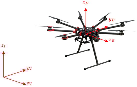
Figure 1.
Reference frames for the UAV (DJI S1000). The inertial reference frame is denoted by the subscript , while the body-fixed reference frame is denoted by the subscript .
For the sake of simplicity, we consider a planar problem where the UAV is constrained to move in the plane. The state of the UAV is described through the following generalized coordinates: is the horizontal position of its CoG in the inertial frame, is its vertical position, and is the roll angle (about the axis).
The simplified dynamics of the UAV [16] are described by the following equations:
where and are the thrust control force and the rolling control torque exerted by the propellers, respectively, and is the gravitational acceleration.
These control actions are determined through a PID controller, which aims to minimize the UAV vertical displacement and roll angle, i.e., correct any deviations from the hovering state. The PID controller equations are as follows:
It has to be noticed that, since multicopters are underactuated systems, the horizontal position of the UAV cannot be controlled independently but only by applying a combination of thrust force and roll torque. The coefficients of the PID controller used in the simulations are summarized in Table 1 [9].

Table 1.
Coefficients of the UAV PID controller.
The UAV base, in addition to the reaction torque and force due to the movement of the manipulator, is subject to the action of the following external forces:
- Gravity ();
- The net thrust, and roll torque, determined by the control law (exerted through the propellers);
- Aerodynamic disturbances (, modeled in Section 4).
The generalized coordinates and the external forces/torques (except the manipulator reaction force/torque) acting on the UAV are illustrated in Figure 2.
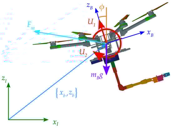
Figure 2.
Generalized coordinates, reference frames, and external forces/torques applied to the UAV. Control forces are in red, gravity force is in purple, and aerodynamic force is in cyan.
2.2. Kinematics of Flying-Base Manipulators
In our model, a planar serial manipulator with revolute joints is mounted on the UAV. The axes of the revolute joints are perpendicular to the working plane. The first revolute joint (the one that connects the manipulator to the base) is vertically aligned with the UAV CoG, at a distance .
The configuration of the robotic manipulator is described by the vector of joint angles, , where is the number of the manipulator degrees of freedom (DOFs). We denote with the length of the -th link and with the distance between joint and the CoG of link . The first revolute joint is joint 0. We assume the barycenters to be exactly in the middle of links, so that .
Figure 3 illustrates the symbols just introduced.
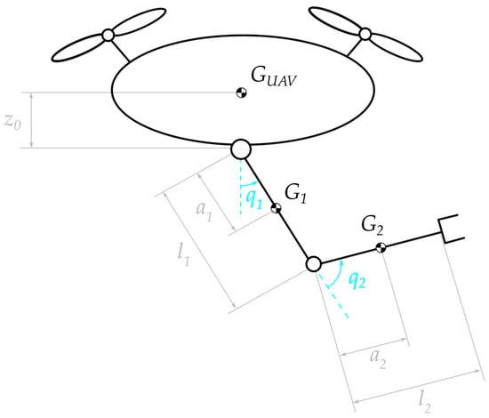
Figure 3.
Schematic illustration of the aerial manipulator and its geometrical parameters.
The inverse kinematics method we propose is based on the inverse kinematics formula for floating-base systems. In these systems, both the joint and the base velocities contribute to the end-effector velocity. The relationship between these velocities is described by the differential kinematics equation [10]:
where is the manipulator Jacobian matrix, is the base Jacobian matrix, is the vector of the linear and angular end-effector velocities, is the vector of the joint velocities, and is the vector of the base velocities. Equation (3) can be differentiated to express the relationship between the end-effector accelerations and the base/joint velocities and accelerations, enabling a solution of the inverse kinematics at the acceleration level:
For the trajectory tracking problem, we aim to follow a given end-effector velocity (or acceleration) profile. The inverse kinematics can be solved by a time discretization: at each timestep, the end-effector velocity is known, and the joint velocities are calculated by exploiting the differential kinematics equations. For fixed-base manipulators, the base velocities and accelerations are null; therefore, the inverse kinematics problem can be solved by inverting Equations (3) and (4), after the computation of the inverse of [17]. This is not sufficient for mobile-base manipulators. In this case, the velocities and accelerations of the base can be significant and must be known in order to solve the inverse kinematics problem. In the methods we present, the base motion is computed from the external forces that act on the system. Therefore, the dynamics of the system have to be considered in order to solve its inverse kinematics.
2.3. Dynamics of Flying-Base Manipulators
The dynamic model of a flying-base manipulator can be expressed in matrix form by the following equations (for more details see [18]):
where the variables are as follows:
- represents the base inertia matrix;
- represents the base–manipulator coupling inertia matrix;
- represents the manipulator inertia matrix;
- are velocity-dependent non-linear terms (Coriolis and centrifugal terms);
- is the total force/torque applied to the base;
- is the vector of the joint torques;
- is the external force/torque on the end-effector.
The inertia matrices above can also be used to express the relationship between the base and joint velocities () and the total momentum of the system () [19]:
where represent the linear and angular momentum of the system, respectively. The angular momentum is calculated with respect to the UAV CoG ().
The differentiation of the momentum formula (6) yields the following acceleration constraint:
which introduces a relationship between the system generalized velocities/accelerations and the rate of change in the total momentum, (which is directly related to the external forces/torques, acting on the system; see Equation (12) in the following section).
3. CLIK Algorithms for UAM Control
The equations developed in the previous section can be employed to build a CLIK [11] control algorithm for aerial manipulators. CLIK algorithms are a family of control strategies designed to solve the differential inverse kinematics problem for robotic manipulators in the presence of numerical drift, modeling errors, and/or unknown disturbances [17].
These kinematic control schemes calculate the joint trajectories necessary to follow an assigned end-effector trajectory [20,21]. These then constitute the reference input to some joint feedback control scheme that is not modeled in this work.
The two methods presented in this paper use the differential kinematics Formulas (3) and (4) to solve the inverse kinematics. The first method (Section 3.1) solves the inverse kinematics at the velocity level and is called the first-order algorithm, while the second one (Section 3.2) solves the inverse kinematics at the acceleration level and is called the second-order algorithm.
3.1. Velocity-Level CLIK Algorithm for UAMs
The first algorithm we present is designed to compute the joint velocities required to obtain the desired end-effector velocity, .
The method can be seen as the closed-loop version of the Generalized Jacobian method, originally developed for space robotic manipulators mounted on a floating base and modified in [9] for aerial manipulator control. It has to be noticed that in the case of aerial manipulators, it is necessary that the algorithm also takes into account the effect of external forces (effect that is instead negligible for space manipulators, for which the conservation of momentum assumption can be exploited).
The joint velocities can be derived from (3):
In order to find the joint velocities, the base velocity, is required. This can be expressed as a function of the joint velocities and the linear and angular momenta of the system using Equation (6):
Inserting Equation (9) into Equation (3), we obtain the following equation:
The matrix is called Generalized Jacobian matrix and is represented as . This matrix is the generalization of the usual Jacobian matrix (i.e., the one used for fixed-base manipulators) in the case of flying-base manipulators. It has to be noticed that, if the linear and angular momenta of the system are null and conserved, Equation (10) is formally analogous to the differential kinematics equation for fixed-base manipulators (). Given the definition of the Generalized Jacobian, Equation (8) can be rewritten as follows:
The linear and angular momenta of the system can be calculated from the principles of dynamics. In particular, the rate of change in the linear and angular momenta is related to the external forces ( and torques () acting on the system through the following equation:
where the subscript denotes the point about which the angular momentum is computed, and is the velocity of this point. In this work, the angular momentum is computed with respect to the UAV CoG, and the velocity of this point is called . Integrating (12) over time, the linear and angular momenta at time can be computed from the given momenta at time as follows:
The algorithm is implemented in discrete time in the controller. At each timestep, Equation (13) assume the following form:
The external forces/torques that are considered in the computation of the momenta and are the gravity force, and the control force and the control torque generated by the propellers. To make the computation, we define the following vectors:
- : vector from the origin of the inertial frame to the base CoG, ;
- : vector from the origin of the inertial frame to the whole system CoG, .
The external force can be computed through the following equation:
where is the rotation matrix from the base frame to the inertial frame and is the total mass of the UAM. The external torque (computed with respect to the base CoG, ) is as follows:
While the gravity and control forces can be predicted with good accuracy, other disturbances, such as aerodynamic ones, are difficult to estimate. If the estimation of these external forces/torques is incorrect, then the linear and angular momenta will not be updated correctly, and the error will propagate to joint velocities, affecting the position of the end-effector. Moreover, in real-world application scenarios, the accuracy of the computation of the Generalized Jacobian is affected by the errors in the estimation of the inertial parameters and state of the UAM, thus affecting the computation of the joint velocities (through Equation (11)).
In order to compensate for this position error, a feedback correction term, is added when computing the joint velocities. Therefore, the following equation applies:
where represents the velocities calculated through Equation (11). The feedback term is based on the task-space error, which is defined as , where is the desired position of the end-effector and is its actual position. The feedback correction term is calculated as follows:
where is a diagonal, square, and positive definite matrix of gains. Therefore, the fundamental formula of the velocity-level CLIK algorithm for UAMs can be written as follows:
This method is implemented recursively by a time discretization. At each timestep, the joint velocities are computed by the discretized form of (19):
The joint velocities are integrated numerically to find the joint angles, , which are then used to compute the end-effector position, through forward kinematics. In Equation (20), the matrices , , and and the task-space error, are computed using the joint angles and the end-effector position from the previous timestep, momenta and are calculated as shown in Equation (14), and is known from the desired trajectory.
In the case of a redundant manipulator, the Generalized Jacobian is not a square matrix and cannot be inverted. However, a minimum joint velocity solution can be found replacing the inverse of the Generalized Jacobian with its pseudoinverse in Equation (19). In this case, it is also possible to adopt the method of the Extended Generalized Jacobian or the null-space projection method developed in [9] and [8], respectively.
In order to calculate the task-space error and thus the feedback term, it is necessary to know the actual position, of the end-effector, which must be compared with the desired position, . In the controller implemented in the simulator, is computed through forward kinematics. In real experiments, it is better to obtain through sensor measurements (e.g., through a vision system) so that the algorithm is not influenced by uncertainties in the kinematic model of the system.
By comparing this algorithm with the algorithms proposed in [12,15], it is worth noticing that our method includes the dynamics of the system in the inverse kinematics equation through the use of the Generalized Jacobian and updating the linear and angular momenta with known generalized forces (see Equation (14)). On the other hand, the previous methods only include the effect of the UAV state on the Jacobian [15], or they compute the Jacobian for fixed-base manipulators [12].
3.2. Acceleration-Level CLIK Algorithm for UAMs
In this subsection, we present a novel and more sophisticated approach based on the work done for space manipulators kinematic control [22], which allows us to solve flying-base robotic systems inverse kinematics at the acceleration level.
We assume that the trajectory of the end-effector is given through its acceleration profile, , and that the generalized external forces, acting on the system are known. The momentum in Equation (7) can be rearranged to obtain the following acceleration constraint:
where is the vector containing the derivatives of the linear and angular momenta. Since we consider the angular momentum about the CoG of the base, which is a moving point, its derivative is (where and represent the linear velocity of the base CoG and that of the entire system CoG, respectively). Along with (21), we consider the kinematic Equation (4), which can be rearranged as follows:
Equations (21) and (22) can be put together to form the following linear system:
For a UAM with an -DOF manipulator, the matrix in the above equation is of dimensions . If all the external forces and torques acting on the system can be estimated accurately so that the term is sufficiently reliable, the inversion of Equation (23) leads to open-loop inverse kinematic control at the acceleration level:
If the manipulator is redundant, the solution can be obtained by using the pseudoinverse instead of the inverse of the matrix in (24).
The accurate prediction of the external forces on the system is difficult. Therefore, a more reliable control scheme can be obtained by adding a feedback term into the task-space error in :
As we are operating at the acceleration level, the feedback term can include a derivative action based on the end-effector velocity error, . The gain matrices and are diagonal and positive definite. The joint velocities, inside can be measured through sensors. The linear and angular velocities of the base, , can be measured or computed from the following momentum constraint (6):
For calculating we notice from Equation (22) that this term is equal to the acceleration of the end-effector when the generalized accelerations (, ) are null:
This acceleration is calculated through the forward recursion of the Newton–Euler recursive scheme for solving free-base manipulators inverse dynamics [22]. On the other hand, the term can be computed from Equation (21):
where corresponds to the total momentum of the system when the generalized accelerations are null.
As for the algorithm presented in Section 3.1, this inverse kinematics algorithm considers the dynamics of the UAM, now through the constraint described by Equation (21). Other CLIK algorithms presented in the literature (such as the one in [13]) only consider the geometry and state of the UAM.
4. Simulation Setup
The CLIK control algorithms described in the previous sections are implemented in a MATLAB dynamic simulator, which recursively solves the kinematics and dynamics of free-base robotic systems. The simulator was originally developed for space manipulators [23] and now has been adapted to also take into account external forces such as UAV control forces/torques, gravity, and aerodynamic disturbances that usually act on UAMs.
The MATLAB simulator code consists of two modules that run subsequently at each timestep (in all the simulations, the step size is ). The first module represents the kinematic controller; it computes either the joint velocities or accelerations (depending on which CLIK algorithm is employed) to attain the desired velocity/acceleration of the end-effector. In the second module, first, the inverse dynamics of the system is solved to determine the required joint torques for executing the specified motion. Then, the system direct dynamics is solved.
Simulations are carried out for UAMs with two-DOF and three-DOF planar robotic arms moving in the plane. Moreover, the planar dynamic model of the UAV presented in Section 2.1 is used. In this case, since the base of the UAM cannot move in the direction and the desired trajectory of the end-effector lies on the plane, the system is planar and, therefore, the CLIK algorithms presented in Section 3 are simplified accordingly.
Thanks to the simulator, it is possible to execute several simulation experiments to evaluate the performance of the different CLIK control algorithms presented in this paper. As a measure of the system performance, we choose the 2-norm difference between the desired and actual end-effector position over time, i.e., the end-effector position error norm.
Two types of simulation experiments are presented. The first type is aimed at testing the trajectory tracking performance of the system in the presence of unpredictable disturbances. In these experiments, the UAM objective is to track a circular trajectory of diameter m and to complete it in a time s. The trajectory is to be tracked following the curvilinear abscissa profile, shown in Figure 4 (refer to [24] for more details on how the profile is generated). After time , the end-effector is required to stand still at the final point for a time = 1 s.
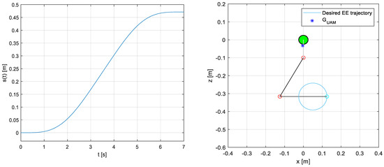
Figure 4.
(left) Curvilinear abscissa, of end-effector desired trajectory as a function of time; (right) UAM initial configuration in the x–z plane. The green circle represents the UAV CoG, and the blue star represents the whole system CoG, . In cyan, the desired circular trajectory to be tracked by the end-effector is shown.
The second type of experiment is used to evaluate the system ability to reject disturbances that might come from the end-effector interaction with the environment. In these experiments, the UAM is subject to an impulsive force applied to its end-effector after having completed a horizontal linear trajectory. This force simulates a disturbance that might come from the environment, such as a collision with an object.
In each simulation, the initial conditions for the joints are set so that the base and UAM CoGs are almost aligned vertically (with a maximum tolerance of +/−5 mm), the manipulator is in a non-singular configuration, and the system is in equilibrium with a control force and torque keeping the UAM in a hovering state. The starting point of the end-effector is set to the beginning of the specified trajectory, while the initial position of the base CoG is set at point of the inertial frame. The initial configuration of the system is shown in Figure 4.
The UAV and manipulator geometrical and inertial characteristics are presented in Table 2.
Table 2.
Geometrical and inertial characteristics of the UAM used in the simulation experiments.
In order to simulate a realistic scenario in the simulator, three sources of disturbance are modeled:
- Aerodynamic disturbances;
- Sensors noise in the measurements of the UAV linear and angular positions and velocities used in the inverse kinematics;
- Incorrect inertial parameters in the model used for the computation of the inverse kinematics.
4.1. Aerodynamic Disturbance Model
In real operative scenarios, wind is a typical cause of undesired motion of the UAV and thus can be a source of error in the positioning of the end-effector. For this reason, a model of this disturbance is implemented in the simulator.
Most aerodynamic disturbance models on UAVs that can be found in the literature are based on empirical formulas with coefficients that come either from data derived from expensive experiments on UAVs or from sophisticated CFD simulations (see, for example, [25,26]). The purpose here is to have a simple model of disturbance to test the rejection capabilities of the proposed inverse kinematics control algorithms. We therefore model the aerodynamic disturbance as a random concentrated force acting on the UAV CoG due to wind. First, a wind speed profile is generated using the well-known Dryden model [27], and then a simple model is used to associate the wind speed profile with the force on the base.
4.1.1. Wind Speed Profile Generation
The wind velocity vector, which has a horizontal and vertical component, can be modeled as the sum of two vectors [28]:
with representing the static wind vector (which represents the mean value of the overall wind vector) and representing the fast time-varying (or gust) component. This last component features higher frequencies and smaller amplitudes in comparison with the static wind vector. Since our goal is to test the performance of the system under a dynamic load, we neglect the static component.
The behavior of the wind gust component, follows the Dryden model, which defines the horizontal and vertical () components of wind as a sum of sinusoidal components:
where the generic subscript is adopted in lieu of the subscripts or . In Equation (30), and are randomly selected frequencies and phase shifts, is the number of sinusoids, and are the amplitudes of the sinusoids. For realistic results, it is suggested to consider between 0.1 and 1.5 rad/s. For simplicity, we select equally spaced frequencies in this range for both horizontal and vertical components (). The amplitudes, are given by the following equation:
where is the interval between the chosen frequencies, and is a Power Spectral Density (PSD) function evaluated for . The PSD expressions for the horizontal and vertical wind components are different and are defined in the Dryden model, respectively, as follows:
where and are the horizontal and vertical turbulence intensities, and and are the horizontal and vertical gust length scales. As suggested in [29], the vertical length scale and the turbulence intensity can be assumed to be (where is the altitude of the UAV) and ( is the given wind speed in knots at a 20 ft altitude). In [30], it is suggested to use knots for light turbulence. Finally, and are found with the following equations, where the parameters are modified to allow us to have the altitude input, expressed in SI units:
The altitude at which the UAM operates is set to .
4.1.2. Aerodynamic Force on the UAV
The wind velocity can be calculated through Equations (30)–(33). In order to compute the aerodynamic force acting on the UAV due to the wind velocity, the model described in [31] is adopted. This model has the advantage of being simple to implement compared to other ones that can be found in the literature. The model gives the intensity of the force exerted on the UAV, as a function of the wind velocity:
where is the effective area of influence, and [27]. For simulation purposes, we use the components of Formula (34) as projections on the axes of the inertial frame:
where is the inclination angle of the wind velocity vector with respect to the horizontal, and and represent the projections of the effective area on the planes perpendicular to the and axes, respectively. For simplicity’s sake, the UAV is represented as a cylinder in the computation of the effective area. The expressions of the effective area projections are as follows [31]:
where and are the pitch and roll angles, respectively, and are the fill factors for the cylinder area (introduced to take into account that the UAV does not fill the entire cylindrical volume in which we inscribe it, and they depend on the UAV design), is the cylinder radius, and is the cylinder height. The parameters used in Formula (36) are listed in Table 3. The values of the fill factors and are derived from the DJI S1000 CAD model.
Table 3.
Parameters in Formula (36).
In this work, the roll angle variations are small and, therefore, we assume that remains constant. Force profiles associated with the wind speed profiles of Figure 5 are shown in Figure 6.
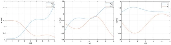
Figure 5.
Examples of wind velocity profiles generated through the Dryden model ( and rad/s). In blue, the horizontal wind velocity component is shown, and in orange, the vertical wind velocity component is shown. (left) Example 1; (middle) Example 2; (right) Example 3.
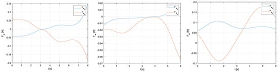
Figure 6.
Horizontal (in blue) and vertical (in orange) force profiles associated with the wind velocity profiles of Figure 5. (left) Example 1 (force profiles acting in the simulations presented in the following sections); (middle) Example 2; (right) Example 3.
4.2. Sensors Noise
The kinematic control methods proposed in this paper need to have the position, attitude, and velocities of the UAV base as inputs. There are different combinations of sensors that can be used to obtain these data. Typically, sensor fusion techniques are used to obtain the best estimate of the pose of the vehicle [32].
The base position can be measured by resorting to GPS (few centimeters of accuracy at a rate of up to 10 Hz) in outdoor environments or to external localization devices such as a VICON motion capture system (very high accuracy at about 200 Hz) or on-board camera-based systems (few centimeters of accuracy at about 20–50 Hz) [33]. As for attitude measurements, most of the UAVs today have an inbuilt IMU (Inertial Measurement Unit) equipped with three-axis gyroscopes, providing measurements of the attitude rates; three-axis accelerometers, providing measurements of the accelerations; and a magnetometer, providing the absolute heading.
In real experiments, measurements from sensors are affected by noise. Therefore, noisy measures of the base linear and angular positions and their velocities, which are used in the inverse kinematics methods proposed, can affect the capability to accurately track a trajectory with the end-effector. In order to simulate the measured data in a realistic way in our simulator, normally distributed measurement noise with a null mean was added to the simulated measurements coming from the UAV. In particular, in the simulator, the noise is added to the measured variables (i.e., those estimated by the direct dynamics module), which are then used as inputs for the inverse kinematics module.
The standard deviations of the noise corrupting each measurement used in this work are listed in Table 4.
Table 4.
Standard deviations of the distributed noise added to the considered measurements.
4.3. Inertial Parameters Uncertainty
In order to test the robustness of the kinematic controller to parameters uncertainty, we consider the possibility of using inertial parameters that differ from the reference values used in the dynamic simulation. The parameters taken into consideration are the UAV and link masses () and moments of inertia (). We assign to each parameter a realistic possible variation (expressed as a percentage of the reference value) because the real parameters can differ from the nominal ones. For example, a +/−15% possible variation is chosen for the mass, , and the moment of inertia, , of the UAV, considering that these can vary greatly depending on the effective on-board instrumentation and how it is positioned on the UAV frame. The assumed variations in the inertial parameters between the ones used in the kinematic controller and their reference values are listed in Table 5.
Table 5.
Assumed variation in the inertial parameters used in the kinematic controller compared to those used in the dynamic simulations (reference values).
5. Simulation Results
In this section, we report the results of the trajectory tracking and disturbance rejection tests carried out with the dynamic simulator described in Section 4. We first show the performance of the velocity-level algorithm and then the performance of the acceleration-level one. The results for the trajectory tracking tests are shown for both an aerial manipulator with a two-DOF arm (as described in Section 4) and one with a three-DOF arm. In the latter case, one link is added with the same geometrical and inertial characteristics as the other two. The three-DOF manipulator is kinematically redundant since the task involves the tracking of a two-DOF trajectory with the end-effector (its orientation is not controlled).
For each of the two kinematic control algorithms, we first show their performance in an open-loop scenario (joint reference velocity or acceleration profiles given by the inverse kinematics solution) and then in the case with the feedback, introduced to reduce the end-effector error to zero. To make the results comparable, we assume that the aerodynamic disturbances have the same behavior (depicted in the first graph of Figure 6) in all the simulations carried out. In all of them, we also assume that the kinematic controller uses inertial parameters of the UAM that differ from the nominal ones as described in Section 4.3 (the maximum positive variation is always considered).
In the disturbance rejection tests, the only unknown force acting on the system is the impulsive force on the end-effector. Experiments are carried out only for a two-DOF arm.
For each experiment, we report the temporal evolution of the norm of the task-space error (the end-effector error) and the trajectories of the end-effector and the base COG. The joint position, velocity, or acceleration limits are not considered in this work, and the inclusion of them could be part of future work.
5.1. Velocity-Level Algorithm Results
5.1.1. Trajectory Tracking Results
Figure 7 shows the behavior of the system when controlled through the velocity-level inverse kinematics algorithm in an open-loop scenario (meaning without the feedback term introduced in Section 3). All the disturbances and possible variations in the internal parameters previously described in Section 4 act on the system. It is worth noticing that, even though the use of the Generalized Jacobian adapted to UAMs should predict and compensate for base motions, this method fails to track the desired trajectory because of the presence of disturbances.
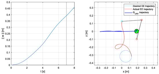
Figure 7.
System response in the case of wind disturbance and sensors noise. The system is controlled by an open-loop velocity-level inverse kinematics algorithm (). The inverse kinematics is solved using the maximum positive variation in all the inertial parameters, see Table 5. (left) Task-space error 2-norm, as a function of time. From the instant , indicated with the black vertical line, the end-effector tries to remain still at the trajectory final point. (right) Graphical output of the simulator in the vertical (x–z) plane; the blue star represents the UAM CoG.
By setting a feedback loop gain of , it can be noticed from Figure 8 that the system can track the trajectory with good accuracy. The sensors noise causes the trajectory to oscillate at a high frequency around the desired one, but the error norm still stays below 5 mm most of the times.
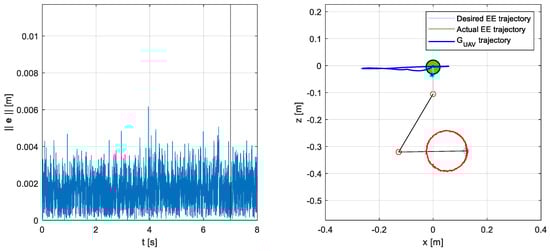
Figure 8.
System response in the case of wind disturbances and sensors noise. The system is controlled by a closed-loop velocity-level inverse kinematics algorithm (). The inverse kinematics is solved using the maximum positive variation in all the inertial parameters, see Table 5. (left) Task-space error 2-norm, , as a function of time. From the instant , indicated with the black vertical line, the end-effector tries to remain still at the trajectory final point. (right) Graphical output of the simulator in the vertical (x–z) plane; the blue star represents the UAM CoG.
Figure 9 shows the performance of the algorithm in controlling an aerial manipulator equipped with a three-DOF arm. Since the orientation of the end-effector is not controlled, the arm is kinematically redundant for this tracking task. The reference velocities of the joints, , are obtained from Equation (19) using the pseudoinverse of the Generalized Jacobian. As in the previous case, .
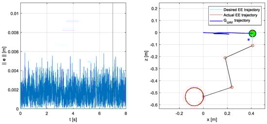
Figure 9.
Three-DOF system response in the case of wind disturbances and sensors noise. The system is controlled by a closed-loop velocity-level inverse kinematics algorithm (). The inverse kinematics is solved using the maximum positive variation in all the inertial parameters, see Table 5. (left) Task-space error 2-norm, , as a function of time. From the instant , indicated with the black vertical line, the end-effector tries to remain still at the trajectory final point. (right) Graphical output of the simulator in the vertical (x–z) plane; the blue star represents the UAM CoG.
5.1.2. Disturbance Rejection Results
Figure 10 shows the response of the system to an impulsive force on the end-effector after a linear horizontal trajectory. The impulse has a triangular shape. Its time duration is 0.2 s, and its maximum value is 12 N. The algorithm shows good robustness against these types of impulsive disturbances, with a positioning error that settles under 0.1 mm about 7 s after the impulse. The algorithm is also tested for lower peak values of the impulse obtaining lower errors and faster rejection dynamics. On the other hand, higher impact forces cause a large UAV horizontal translation, which in turn causes the arm to reach singular configurations and the algorithm to fail.
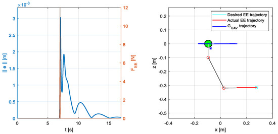
Figure 10.
System response in the case of an impulsive force acting on the manipulator end-effector at the end of a linear trajectory (). The impulse is acting in the negative x direction. The system is controlled by a closed-loop velocity-level inverse kinematics algorithm (). The inverse kinematics is solved using the maximum positive variation in all the inertial parameters, see Table 5. (left) Task-space error 2-norm, (in blue), as a function of time. From the instant , indicated with the black vertical line, the end-effector tries to remain still at the trajectory final point. The orange line indicates the impulsive force, , on the end-effector. (right) Graphical output of the simulator in the vertical (x–z) plane; the blue star represents the UAM CoG.
5.2. Acceleration-Level Algorithm Results
5.2.1. Trajectory Tracking Results
Figure 11 shows the dynamic response of the system controlled through the acceleration-level algorithm with the reference joint acceleration profiles computed by Equation (24). All the disturbances and possible variations in the inertial parameters presented in Section 4 are active, as in the case of the velocity-level algorithm.
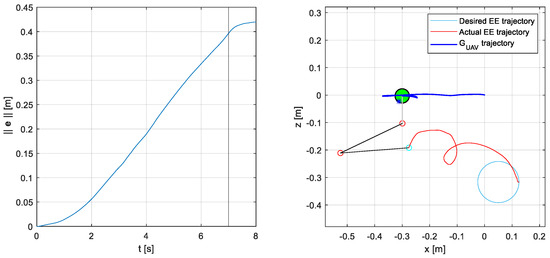
Figure 11.
System response in the case of wind disturbances and sensors noise. The system is controlled by an open-loop acceleration-level inverse kinematics algorithm (). The inverse kinematics is solved using the maximum positive variation in all the inertial parameters, see Table 5. (left) Task-space error 2-norm, , as a function of time. From the instant , indicated with the black vertical line, the end-effector tries to remain still at the trajectory final point. (right) Graphical output of the simulator in the vertical (x–z) plane; the blue star represents the UAM CoG.
Figure 12 shows the dynamic response of the system subject to all the modeled disturbances and variations in the inertial parameters when controlled by the closed-loop acceleration-level algorithm. The proportional and derivative gains are set to and .
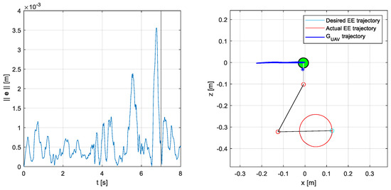
Figure 12.
System response in the case of wind disturbances and sensors noise. The system is controlled by a closed-loop acceleration-level inverse kinematics algorithm (, ). The inverse kinematics is solved using the maximum positive variation in all the inertial parameters, see Table 5. (left) Task-space error 2-norm, (in blue), and force on the end—effector, (in orange), as a function of time. From the instant , indicated with the black vertical line, the end-effector tries to remain still at the trajectory final point. (right) Graphical output of the simulator in the vertical (x–z) plane; the blue star represents the UAM CoG.
It can be noticed that the acceleration-level algorithm ensures good accuracy in tracking the desired trajectory even in the presence of sensors noise: the maximum error norm is always less than 4 mm. Moreover, the actual end-effector trajectory is significantly smoother with respect to that of the velocity-level algorithm.
Finally, in Figure 13, the performance of the algorithm in controlling a UAM with a three-DOF arm is shown. In this case, the error is slightly larger but still acceptable in real-world application scenarios.
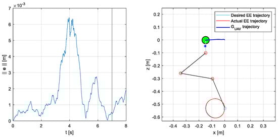
Figure 13.
Three-DOF system response in the case of wind disturbance and sensors noise. The system is controlled by a closed-loop acceleration-level inverse kinematics algorithm (, ). The inverse kinematics is solved using the maximum positive variation in all the inertial parameters, see Table 5. (left) Task-space error 2-norm, , as a function of time. From the instant , indicated with the black vertical line, the end-effector tries to remain still at the trajectory final point. (right) Graphical output of the simulator in the vertical (x–z) plane; the blue star represents the UAM CoG.
5.2.2. Disturbance Rejection Results
Figure 14 shows the response of the system to an impulsive force on the end-effector after a linear horizontal trajectory when controlled through the acceleration-level algorithm. The impulse is triangular, with a time duration of 0.2 s and a maximum value of 12 N. In this case, the controller shows more robustness compared to the velocity-level one: the error drops under 0.1 mm just 0.3 s after the impulse.
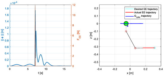
Figure 14.
System response in the case of an impulsive force acting on the manipulator end-effector at the end of a linear trajectory (). The impulse is acting in the negative x direction. The system is controlled by a closed-loop acceleration-level inverse kinematics algorithm (). The inverse kinematics is solved using the maximum positive variation in all the inertial parameters, see Table 5. (left) Task-space error 2-norm, (in blue), as a function of time. From the instant , indicated with the black vertical line, the end-effector tries to remain still at the trajectory final point. The orange line indicates the impulsive force, , on the end-effector. (right) Graphical output of the simulator in the vertical (x–z) plane; the blue star represents the UAM CoG.
Similarly to the velocity-level solution, the algorithm is also tested for lower peak values of the impulse obtaining lower errors and faster rejection dynamics. On the other hand, higher impact forces cause a large UAV horizontal translation, which in turn causes the arm to reach singular configurations and the algorithm to fail.
6. Conclusions
In this paper, we propose two new CLIK algorithms for the kinematic control of aerial manipulators. The first algorithm solves the inverse kinematics at the velocity level and is based on the Generalized Jacobian method with external forces, while the second one solves the inverse kinematics at the acceleration level with a constraint that takes into account the dynamics of the system.
The trajectory tracking effectiveness of both methods is tested in a simulation environment in which the UAM is asked to track a planar circular trajectory. In the simulation environment, the UAV is subject to aerodynamic disturbances caused by wind, and the sensors measurement is corrupted by distributed Gaussian noise. Moreover, the robustness of the algorithms to variations in the inertial parameters of the system with respect to the nominal ones is assessed. Tests are conducted for both a two-DOF aerial manipulator and a (redundant) three-DOF one. Both algorithms prove to be effective in controlling the aerial manipulator subject to wind action with similar performances. On the other hand, the acceleration-level algorithm shows significantly better performance in handling measurements corrupted by Gaussian noise: the tracking error is smaller, and the end-effector trajectory is smoother.
To test the system robustness to disturbances that might come from the environment, such as collisions with objects, we perform simulated experiments in which the UAM experiences an impulse-type force at its end-effector after the execution of a linear trajectory. Both algorithms show good overall performance, with the acceleration-level algorithm showing a smaller settling time.
In the dynamic simulations, the base undergoes noticeable translations and rotations during the execution of the tasks. This could cause problems if, in a real context, the UAM operates close to obstacles or in close proximity to walls. In the future, new solutions must be explored to supplement the algorithms developed in this research with methods to minimize the base movements. For example, additional tasks could be included in the kinematics inversion if the UAM arm is redundant, or a controlled mobile counterweight could be used to balance the gravity torque. Further future developments of this work will include improving the algorithms in order to produce only motions within specified joint physical limits, extending the control algorithms to three-dimensional systems, and experimentally validating them in real-world application scenarios. The theoretical proof of the stability of the proposed control methods will also be part of future work.
Author Contributions
Conceptualization, S.C.; methodology, S.C., G.F. and M.P.; software, S.C., A.P. and M.P.; formal analysis S.C., A.P. and M.P.; investigation, S.C., A.P. and M.P.; writing—original draft preparation, A.P. and M.P.; writing—review and editing, A.B., S.C., G.F., A.P. and M.P.; supervision, project administration, and funding acquisition, S.C. All authors have read and agreed to the published version of the manuscript.
Funding
This work was carried out in the framework of the project “DynAeRobot—Development and validation of a new dynamically balanced aerial manipulator” (project no. BIRD213590), funded under the BIRD 2021 program promoted by the University of Padova.
Institutional Review Board Statement
Not applicable.
Informed Consent Statement
Not applicable.
Data Availability Statement
The original contributions presented in the study are included in the article, and further inquiries can be directed to the corresponding author.
Conflicts of Interest
The authors declare no conflicts of interest.
References
- Bonyan Khamseh, H.; Janabi-Sharifi, F.; Abdessameud, A. Aerial Manipulation—A Literature Survey. Robot. Auton. Syst. 2018, 107, 221–235. [Google Scholar] [CrossRef]
- Ruggiero, F.; Lippiello, V.; Ollero, A. Aerial Manipulation: A Literature Review. IEEE Robot. Autom. Lett. 2018, 3, 1957–1964. [Google Scholar] [CrossRef]
- Ollero, A.; Tognon, M.; Suarez, A.; Lee, D.; Franchi, A. Past, Present, and Future of Aerial Robotic Manipulators. IEEE Trans. Robot. 2022, 38, 626–645. [Google Scholar] [CrossRef]
- Suarez, A.; Sanchez-Cuevas, P.; Fernandez, M.; Perez, M.; Heredia, G.; Ollero, A. Lightweight and Compliant Long Reach Aerial Manipulator for Inspection Operations. In Proceedings of the 2018 IEEE/RSJ International Conference on Intelligent Robots and Systems (IROS), Madrid, Spain, 1–5 October 2018; pp. 6746–6752. [Google Scholar]
- Suarez, A.; Sanchez-Cuevas, P.J.; Heredia, G.; Ollero, A. Aerial Physical Interaction in Grabbing Conditions with Lightweight and Compliant Dual Arms. Appl. Sci. 2020, 10, 8927. [Google Scholar] [CrossRef]
- Heredia, G.; Jimenez-Cano, A.E.; Sanchez, I.; Llorente, D.; Vega, V.; Braga, J.; Acosta, J.A.; Ollero, A. Control of a Multirotor Outdoor Aerial Manipulator. In Proceedings of the 2014 IEEE/RSJ International Conference on Intelligent Robots and Systems, Chicago, IL, USA, 14–18 September 2014; pp. 3417–3422. [Google Scholar]
- Huang, P.; Xu, Y.; Liang, B. Dynamic Balance Control of Multi-Arm Free-Floating Space Robots. Int. J. Adv. Robot. Syst. 2005, 2, 13. [Google Scholar] [CrossRef]
- Vyas, Y.; Pasetto, A.; Ayala-Alfaro, V.; Massella, N.; Cocuzza, S. Null-Space Minimization of Center of Gravity Displacement of a Redundant Aerial Manipulator. Robotics 2023, 12, 31. [Google Scholar] [CrossRef]
- Pasetto, A.; Vyas, Y.; Cocuzza, S. Zero Reaction Torque Trajectory Tracking of an Aerial Manipulator through Extended Generalized Jacobian. Appl. Sci. 2022, 12, 12254. [Google Scholar] [CrossRef]
- Umetani, Y.; Yoshida, K. Resolved Motion Rate Control of Space Manipulators with Generalized Jacobian Matrix. IEEE Trans. Robot. Autom. 1989, 5, 303–314. [Google Scholar] [CrossRef]
- Siciliano, B. A Closed-Loop Inverse Kinematic Scheme for On-Line Joint-Based Robot Control. Robotica 1990, 8, 231–243. [Google Scholar] [CrossRef]
- Cataldi, E.; Muscio, G.; Trijillo, M.A.; Rodriguez, Y.; Pierri, F.; Antonelli, G.; Caccavale, F.; Viguria, A.; Chiaverini, S.; Ollero, A. Impedance Control of an aerial-manipulator: Preliminary results. In Proceedings of the 2016 IEEE/RSJ International Conference on Intelligent Robots and Systems (IROS), Daejeon Convention Center, Daejeon, Republic of Korea, 9–14 October 2016. [Google Scholar]
- Pierri, F.; Muscio, G.; Caccavale, F. An adaptive hierarchical control for aerial manipulators. Robotica 2018, 36, 1527–1550. [Google Scholar] [CrossRef]
- Sànchez, M.I.; Acosta, J.A.; Ollero, A. Integral Action in First-Order Closed-Loop Inverse Kinematics. Application to Aerial Manipulators. In Proceedings of the 2015 IEEE International Conference on Robotics and Automation (ICRA), Seattle, WA, USA, 26–30 May 2015. [Google Scholar]
- Acosta, J.A.; de Cos, C.R.; Ollero, A. Accurate control of Aerial Manipulators outdoors. A reliable and self-coordinated nonlinear approach. Aerosp. Sci. Technol. 2020, 99, 105731. [Google Scholar] [CrossRef]
- Cocuzza, S.; Rossetto, E.; Doria, A. Dynamic Interaction between Robot and UAV in Aerial Manipulation. In Proceedings of the 2020 19th International Conference on Mechatronics—Mechatronika (ME), Prague, Czech Republic, 2–4 December 2020; pp. 1–6. [Google Scholar]
- Siciliano, B.; Sciavicco, L.; Villani, L.; Oriolo, G. Robotics: Modelling, Planning and Control; Springer Publishing Company: New York, NY, USA, 2010; ISBN 978-1-84996-634-4. [Google Scholar]
- Wilde, M.; Kwok Choon, S.; Grompone, A.; Romano, M. Equations of Motion of Free-Floating Spacecraft-Manipulator Systems: An Engineer’s Tutorial. Front. Robot. AI 2018, 5, 41. [Google Scholar] [CrossRef] [PubMed]
- Yoshida, K.; Umetani, Y. Control of Space Manipulators with Generalized Jacobian Matrix. In Space Robotics: Dynamics and Control; Xu, Y., Kanade, T., Eds.; The Kluwer International Series in Engineering and Computer Science; Springer: Boston, MA, USA, 1993; pp. 165–204. ISBN 978-1-4615-3588-1. [Google Scholar]
- Antonelli, G.; Chiaverini, S.; Fusco, G. Kinematic Control of Redundant Manipulators with On-Line End-Effector Path Tracking Capability Under Velocity and Acceleration Constraints. IFAC Proc. Vol. 2000, 33, 183–188. [Google Scholar] [CrossRef]
- Caccavale, F.; Siciliano, B. Kinematic Control of Redundant Free-Floating Robotic Systems. Adv. Robot. 2001, 15, 429–448. [Google Scholar] [CrossRef]
- Mukherjee, R.; Nakamura, Y. Formulation and Efficient Computation of Inverse Dynamics of Space Robots. IEEE Trans. Robot. Autom. 1992, 8, 400–406. [Google Scholar] [CrossRef]
- Cocuzza, S.; Pretto, I.; Debei, S. Least-Squares-Based Reaction Control of Space Manipulators. J. Guid. Control Dyn. 2012, 35, 976–986. [Google Scholar] [CrossRef]
- Cocuzza, S.; Pretto, I.; Debei, S. Reaction Torque Control of Redundant Space Robotic Systems for Orbital Maintenance and Simulated Microgravity Tests. Acta Astronaut. 2010, 67, 285–295. [Google Scholar] [CrossRef]
- Kuantama, E.; Tarca, R. Correction of Wind Effect on Quadcopter. In Proceedings of the 2018 International Conference on Sustainable Information Engineering and Technology (SIET), Malang, Indonesia, 10–12 November 2018; pp. 257–261. [Google Scholar] [CrossRef]
- Schiano, F.; Alonso-Mora, J.; Rudin, K.; Beardsley, P.; Siegwart, R.; Sicilianok, B. Towards Estimation and Correction of Wind Effects on a Quadrotor UAV. In Proceedings of the IMAV 2014: International Micro Air Vehicle Conference and Competition 2014, Delft, The Netherlands, 12–15 August 2014; pp. 134–141. [Google Scholar]
- MIL-F-8785 C Flying Qualities Piloted Airplanes. Available online: http://everyspec.com/MIL-SPECS/MIL-SPECS-MIL-F/MIL-F-8785C_5295/ (accessed on 5 September 2023).
- Escareño, J.; Salazar, S.; Romero, H.; Lozano, R. Trajectory Control of a Quadrotor Subject to 2D Wind Disturbances. J. Intell. Robot Syst. 2013, 70, 51–63. [Google Scholar] [CrossRef]
- Waslander, S.; Wang, C. Wind Disturbance Estimation and Rejection for Quadrotor Position Control. In AIAA Infotech@Aerospace Conference; Infotech@Aerospace Conferences; American Institute of Aeronautics and Astronautics: Seattle, WA, USA, 2009. [Google Scholar]
- Generate Continuous Wind Turbulence with Dryden Velocity Spectra—Simulink—MathWorks Italia. Available online: https://it.mathworks.com/help/aeroblks/drydenwindturbulencemodelcontinuous.html (accessed on 6 September 2023).
- Viktor, V.; Valery, I.; Yuri, A.; Shapovalov, I.; Beloglazov, D. Simulation of Wind Effect on a Quadrotor Flight. ARPN J. Eng. Appl. Sci. 2015, 10, 1535–1538. [Google Scholar]
- Orsag, M.; Korpela, C.; Oh, P.; Bogdan, S. Aerial Manipulation; Springer: Berlin/Heidelberg, Germany, 2018. [Google Scholar] [CrossRef]
- Arleo, G.; Caccavale, F.; Muscio, G.; Pierri, F. Control of Quadrotor Aerial Vehicles Equipped with a Robotic Arm. In Proceedings of the 21st Mediterranean Conference on Control and Automation, Chania, Greece, 25–28 June 2013; pp. 1174–1180. [Google Scholar]
Disclaimer/Publisher’s Note: The statements, opinions and data contained in all publications are solely those of the individual author(s) and contributor(s) and not of MDPI and/or the editor(s). MDPI and/or the editor(s) disclaim responsibility for any injury to people or property resulting from any ideas, methods, instructions or products referred to in the content. |
© 2024 by the authors. Licensee MDPI, Basel, Switzerland. This article is an open access article distributed under the terms and conditions of the Creative Commons Attribution (CC BY) license (https://creativecommons.org/licenses/by/4.0/).