Extending UWOC System Applications through Photon Transmission Dynamics Study in Harbor Waters

Abstract

Underwater wireless optical communication (UWOC) in harbor waters can facilitate real-time monitoring underwater instruments for environmental monitoring, underwater inspection, and maintenance tasks. This study delves into the complex dynamics of UWOC in four distinct harbor waters. The research employs Monte Carlo method incorporated with Fournier–Forand scattering phase function for simulating photon transmission. Key parameters such as the Transmitted full divergence angle, received aperture, and Field of View (FOV) are meticulously evaluated for their impact on power loss and time delay spread. Notably, the normalized power loss and time delay spread are found to be more significantly affected by communication distance than water quality, and the traditional Beer–Lambert law is ineffective in harbor water. The power loss of Harbor II, III, and IV are found to be 14.00 dB, 31.59 dB, and 41.59 dB lower than that of Harbor I, and the time delay spread of Harbor II, III, and IV is 30.56%, 9.67%, and 0.49% times that of the Harbor I under certain conditions. In addition, increasing the received aperture and FOV, particularly over longer distance, make little contribution to reduce the power loss and mitigate the time delay spread. Based on the fixed transmitted full divergence angle, the most applicable received FOV range is 1–3.2 rad, and the most ideal received aperture is 0.15–0.4 m. Under these conditions, the variation in normalized power loss is less than 2 dB. Additionally, the time delay spread remains within the same order of magnitude with the attenuation length (AL) held constant. These conclusions hold substantial technical relevance for the engineering design of UWOC systems in harbor waters.

1. Introduction

Comprehensive ocean exploration has emerged as a critical focus, garnering significant attentions within scientific, industrial, and military sectors. Key areas such as safety, weather monitoring, and marine commerce are heavily dependent on an in-depth understanding of the marine environment [1]. Yet, exploring this complex terrain, particularly in deep ocean areas, is fraught with challenges. These include high costs, inherent dangers, and technical difficulties. In response to these challenges, there has been rapid advancement in technologies such as underwater wireless sensing, underwater imaging detection, and development of both manned and unmanned underwater vehicles [2]. Consequently, the demand for advanced underwater communication technology, capable of high-rate data transmission, has intensified. Such technology is essential for not only transmitting observational data, but also for gaining a deeper understanding of the marine environment [3].

Underwater wireless communication is a pivotal technology in ocean exploration and operations. Electromagnetic waves, typically employed for communication, face significant attenuation in underwater environment due to the high electrical conductivity of seawater. As a result, sound waves have become the prevalent medium for underwater wireless communication. Despite their ability to cover distances of kilometers, acoustic systems are limited by their transmission bandwidth, typically only reaching speeds of a few Kbps. Moreover, the slow propagation speed of sound underwater poses substantial challenges for real-time, high-speed communication [4]. Further complicating the issue, acoustic communication equipment often suffers from drawbacks such as large size and high energy consumption, which impedes its development and widespread adoption. Finally, certain frequencies of acoustic signals can significantly harm marine organisms, affecting their health, predation behaviors, and migration patterns.

In contrast, underwater wireless optical communication (UWOC) presents several advantages over traditional radio frequency, acoustic communication, and wired communication methods. UWOC is notable for its higher data transmission rates, lower latency, and greater flexibility [5,6,7]. Capable of covering hundreds of meters and potentially achieving Gbps transmission rates, UWOC holds promising application potential in areas such as high-capacity data transmission in deep-sea environments, remote control and monitoring of underwater robotics, and deep-sea oil and gas exploration [8,9,10,11,12]. These advantages position UWOC as a technology with significant potential for advancing the field of underwater communication.

Currently, the mechanical shell of UWOC system in practical applications is predominantly constructed by titanium alloy, an inert metal material. The system’s optical window typically utilizes materials such as sapphire, acrylic, or quartz glass [13]. Additionally, the outer layers of the power supply and network transmission cables are designed to be waterproof, corrosion-resistant, and capable of withstanding pressure. In summary, the materials mentioned above are essentially harmless to aquatic organisms and marine environment in short-term exposure scenarios. Moreover, the light source’s intensity used for communication is generally not excessively high. However, during prolonged underwater operation, marine microorganisms may adhere to the surface of shell and optical window, significantly impairing the communication system’s functionality.

The transmission of light through seawater channels is significantly influenced by dynamic seawater conditions. During transmission, light absorption reduces the total propagation energy, while scattering caused by water particles leads to increased pulse spread in the time domain of the optical signal [14]. Additionally, multiple scatterings result in increased geometric loss in communication links [15]. So, the optical signal’s spatial and temporal distribution characteristics show strong randomness [16]. The high cost of underwater measurement adds the complexity of accurately modeling and analyzing the optical signal variation in underwater channels, a topic that has garnered global research interests [17,18,19,20].

Now the most literature about UWOC predominantly concentrates on light transmission properties and communication technology research in several water types, including clear seawater, coastal seawater, Class Harbor II water, pool water, and laboratory sink water [21,22,23]. The research on different kinds of harbor waters are limited. There are few studies on the transmission characteristics of light in Harbor-I, Harbor-II, Harbor-III and Harbor-IV water. Studying UWOC in harbor water helps in deep understanding how light behaves in such environments and developing techniques to mitigate these effects. Furthermore, harbors are critical infrastructure with high security needs, and UWOC can facilitate real-time monitoring and control of underwater Autonomous Underwater Vehicles (AUVs), sensors, and instruments for environmental monitoring, underwater inspection, and maintenance tasks, which are essential for the sustainable management of harbor areas. Above all, the current engineering application of UWOC systems is mainly under deep sea and ocean water conditions [24,25,26], very little research on laser signal transmission in various harbor waters has limited its wider application.

Furthermore, harbor waters are typically more turbid than the open ocean, primarily due to sediment presence, runoff, and human activities. The myriad substances found in harbor water—including salt, organic compounds, dissolved materials, and potential pollutants—have a profound effect on the light’s absorption and scattering, thereby affecting the absorption of photons [27]. Specifically, higher concentrations of organic matter and suspended particles in harbor waters tend to increase scattering and absorption. The scattering and absorption effects of light are significantly influenced by the size, composition, and concentration of these particles. Additionally, the dynamics of bubble flow in 2D bubble columns can further affect the transmission characteristics of light signals [28]. This is particularly relevant with methane, which is produced by the anaerobic actions of underwater microorganisms and oxygen, generated through the photosynthesis of aquatic plants in harbor waters.

In recent years, the Monte Carlo method has gained popularity for simulating underwater optical signal transmission [29,30,31,32,33,34,35,36]. Gabriel C.’s analysis of underwater channel impulse response and time dispersion across various seawater types, link distances, and received apertures indicates that time dispersion is often negligible, reducing the likelihood of inter-symbol interference [32]. The two-term Henyey–Greenstein Function has been employed for more accurate simulation of power distribution on the receiving surface [29,33]. Shijian Tang’s application of the Monte Carlo method, coupled with the two-term Gamma Function to represent impulse response curves, demonstrates that the two-term Gamma Function model is effective in scenarios with large attenuation lengths [34,35].

Comparing with other types of water, the scattering phase function commonly used at present are not suitable for Monte Carlo simulation in Harbor water, which may lead to incorrect estimation of channel characteristics. The Fournier–Forand scattering phase function has been recognized in recent studies as a better fit for the characteristics of Petzold Harbor water, particularly when compared to the traditional Henyey–Greenstein, two-term Henyey–Greenstein Function, and Sahu and Shanmugam functions [15].

In this study, we would explore the intricate dynamic characteristics of UWOC systems under four distinct Harbor water conditions, which is vital to develop and extend applications in these water conditions. The Monte Carlo method serves as the core simulation technique for modeling photon transport. The rest of the paper is organized in the following manner: Section 2 details the optical parameters of the underwater channel, the selection of an appropriate scattering phase function and the process of the Monte Carlo numerical simulation. Section 3 presents the simulation results and provides a discussion on the normalized power loss and time delay spread as functions of the Transmitted full divergence angle, Received aperture, FOV, and attenuation length (AL). Section 4 concludes the paper with a summary of the findings. This theoretical calculation offers a dependable technical reference for the engineering design of UWOC systems operating in highly turbid waters.

2. Materials and Methods

2.1. The Optical Parameters of the Underwater Channel

The interaction between photons and particles within seawater is both frequent and intense. When a laser beam travels through water, its light is absorbed by various elements such as water molecules, phytoplankton, dissolved organic matter, and organic debris. Concurrently, the light undergoes scattering caused by particles suspended in the seawater [37,38,39]. To mathematically describe these effects, two wavelength-dependent optical characteristic parameters are utilized: the absorption coefficient, denoted as $a\left(\lambda \right)$, and the scattering coefficient, denoted as $b\left(\lambda \right)$. Consequently, the attenuation coefficient, $c\left(\lambda \right)$, which represents the cumulative effect of both absorption and scattering, can be expressed as [40]:

$$c\left(\lambda \right)=a\left(\lambda \right)+b\left(\lambda \right)$$

(1)

$${\omega }_0=b\left(\lambda \right)/c\left(\lambda \right)$$

(2)

In Equation (1), $\lambda$ represents the wavelength of light. The ratio of the scattering coefficient $b\left(\lambda \right)$ to the attenuation coefficient $c\left(\lambda \right)$ is known as the albedo, symbolized as ${\omega }_0$. This ratio, detailed in Equation (2), indicates the proportion of scattering loss relative to the total loss [41,42,43]. For the purpose of this study, which aims to analyze the impact of water turbidity on UWOC, harbor water is categorized into four distinct types: Harbor-I, Harbor-II, Harbor-III, and Harbor-IV. A communication wavelength of 532 nm is chosen for analysis.

Table 1. The optical parameters of four types of Harbor water [44].

Harbor Water Types	$\mathit{a} \left({\mathit{m}}^{-1}\right)$	$\mathit{b} \left({\mathit{m}}^{-1}\right)$	$\mathit{c} \left({\mathit{m}}^{-1}\right)$	${\mathit{\omega }}_0$
Harbor-I	0.187	0.913	1.10	0.83
Harbor-II	0.374	1.826	2.20	0.83
Harbor-III	0.561	2.739	3.30	0.83
Harbor-IV	0.748	3.652	4.40	0.83

presents the absorption coefficient ($a$), scattering coefficient ($b$), attenuation coefficient ($c$), and albedo (${\omega }_0$) for these four types of harbor water. The optical parameters for Harbor II water are sourced from Petzold’s report [38]. For the remaining three Harbor water types, their optical parameters are extrapolated using the same albedo, ${\omega }_0,$ while varying the attenuation coefficients, $c\left(\lambda \right)$.

2.2. Selection of Appropriate Scattering Phase Function

The transmission dynamics of photons in underwater channels are illustrated in Figure 1, Figure 2 and Figure 3. ${\phi }_0$ and ${\mathrm{\psi }}_0$ represent the initial elevation angle and azimuth angle in Figure 1 and Figure 2, respectively. It is important to note that the fixed z-axis is always perpendicular to the Reception Plane. Photons emitted from the light source undergo multiple scatterings by particles within the water, following various trajectories. Some of these photons, termed ‘On-target photons’, reach the photosensitive surface of the receiver and are absorbed, as shown by the blue line. Others, known as ‘Off-target photons’, deviate from the receiver’s aperture and FOV after multiple scatterings shown by the green line, as depicted in Figure 1.

Figure 2 illustrates the multiple scattering events that a photon emitted from the light source undergoes before reaching the Reception Plane. The initial elevation angle and azimuth angle, denoted as ${\phi }_0$ and ${\mathrm{\psi }}_0,$ respectively, correspond to those presented in Figure 1. The angle ${\phi }_1$, ${\phi }_2$, …${\phi }_n$ represent the scattering angles of the photon at each event, while ${\mathrm{\psi }}_1$,${\mathrm{\psi }}_2$, …${\mathrm{\psi }}_n$ denote the azimuth angles associated with these events, with $n$ indicating the $n$-th photon scattering occurrence.

A notable feature in this figure is the gray dotted lines, which depict the photon’s motion coordinate system. This system undergoes continuous transformations with each scattering event, reflecting the dynamic nature of the photon’s path. The specifics of how this coordinate system is determined by the Equation (14). Additionally, it is important to highlight that the x, y, and z axes shown in Figure 2 are part of a fixed coordinate system. This system is established by the positioning of the transmitter and receiver, providing a stable reference frame for understanding the photon’s motion and scattering behavior.

Additionally, the interaction between seawater particles and photons results in two distinct types of light: Forward-scattering light and Backscattering light [21,36], as shown in Figure 3. In the simulation process, the receiver is positioned on the z-axis. The distance between the Transmission Plane and the Reception Plane is governed by a variable known as the attenuation length. The Transmission Plane lies within the x-y plane and is parallel to the Reception Plane, maintaining no angle of declination. This configuration ensures that both the Transmission Plane and Reception Plane are perpendicular to the z-axis, as depicted in Figure 3. This perpendicular arrangement is crucial for accurately simulating the propagation of light or signals in the system and analyzing their interactions with various environmental factors.

In underwater environments, the scattering direction of a photon post-collision with seawater particles is generally random. To evaluate the distribution of light energy following such scatterings, the volume scattering phase function is employed [44,45]. In this study, this function is denoted as $\beta \left(\phi \right)$, the $\phi$ refers to the newly acquired scattering angle in the photon motion coordinate system following a scattering event, it has nothing to do with ${\phi }_0$ and the z axis in Figure 1. Instead, $\phi$ is changing in the photon motion coordinate system, which is constantly changing with each scattering event and is determined by Equation (14). The relationship between the volume scattering phase function and the scattering coefficient $b\left(\lambda \right)$ is articulated in Equation (3) [46]. Here, $\tilde{\beta }(\phi ,\lambda )$ represents the scattering phase function, which plays a crucial role in determining how light is redistributed after interacting with particles in seawater.

$$\left\{\begin{array}{c}1=2\pi {\int }_0^{\pi }\tilde{\beta }(\phi ,\lambda )sin\phi d\phi \\ \tilde{\beta }\left(\phi ,\lambda \right)=\frac{\beta (\phi ,\lambda )}{b\left(\lambda \right)}\end{array}\right.$$

(3)

To date, several scattering phase functions have been proposed to study the light transmission characteristics in underwater channels. Notable among these are the Henyey–Greenstein Function (HG) [46], the two-term Henyey–Greenstein Function (TTHG) [47], Sahu and Shanmugam Function (SS) [46], and the Fournier–Forand Function (FF) [48,49]. The FF scattering phase function, in particular, has been shown to align well with the characteristics of Petzold Harbor water, as indicated in the relevant literature [38].

Further supporting the use of the FF function, simulation results have demonstrated its similarity to the measured data of Petzold Harbor water, especially when specific parameters are applied: a slope (μ) of 3.5835 and a seawater refractive index (n) of 1.13 [15]. Given these findings, this paper adopts the FF scattering phase function for its simulation analysis, and the scattering angle $\phi$ is generated according to the Equation (4), ensuring a direct and unbiased determination of the angle. The expression for the FF scattering phase function is provided in Equation (4). In this expression, $\mathrm{\psi }$ represents the azimuth angle of the photons, and $\phi$ denotes their scattering angle. The variables $\upsilon$ and $\delta$ are intermediate variables without direct physical significance, with ${\delta }_{180}$ representing the value of $\delta$ when the scattering angle $\phi$ equals to 180°.

$$\left\{\begin{array}{c}{\tilde{\beta }}_{FF}\left(\phi \right)=\frac{1}{4\pi {(1-\delta )}^2{\delta }^{\upsilon }}\left\{\upsilon \left(1-\delta \right)-\left(1-{\delta }^{\upsilon }\right)+\left[\delta \left(1-{\delta }^{\upsilon }\right)-\upsilon (1-\delta )\right]{sin}^{-2}\left(\frac{\phi }{2}\right)\right\}+\frac{1-{\delta }_{180}^{\upsilon }}{16\pi \left({\delta }_{180}-1\right){\delta }_{180}^{\upsilon }}(3{cos}^2\mathrm{\psi }-1)\\ \upsilon =\raisebox{1ex}{$(3-\mu )$}\!\left/ \!\raisebox{-1ex}{$2$}\right.\\ \delta =\frac{4}{3{\left(n-1\right)}^2}{sin}^2\left(\frac{\phi }{2}\right)\end{array}\right.$$

(4)

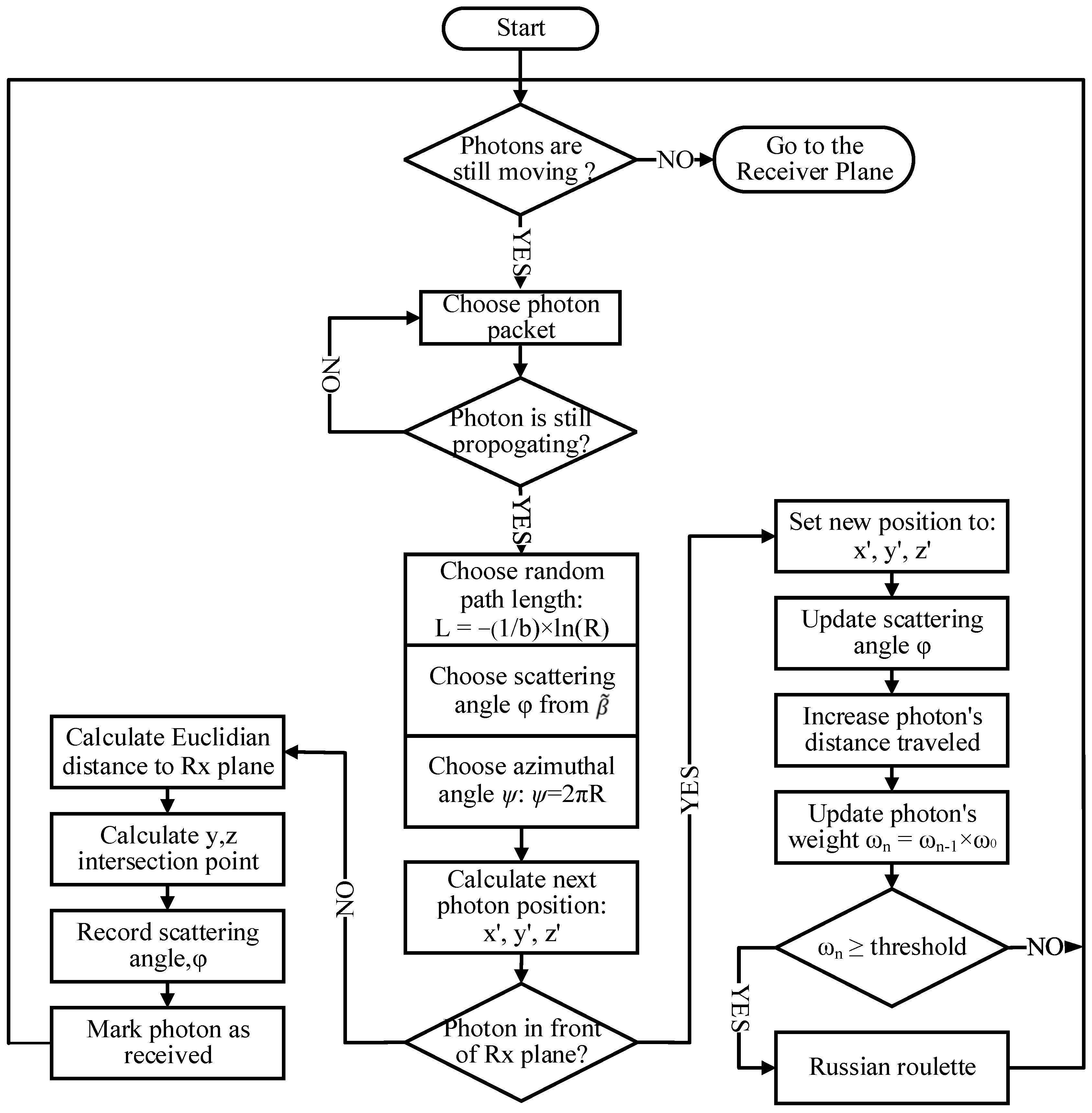
2.3. The Process of Monte Carlo Numerical Simulation

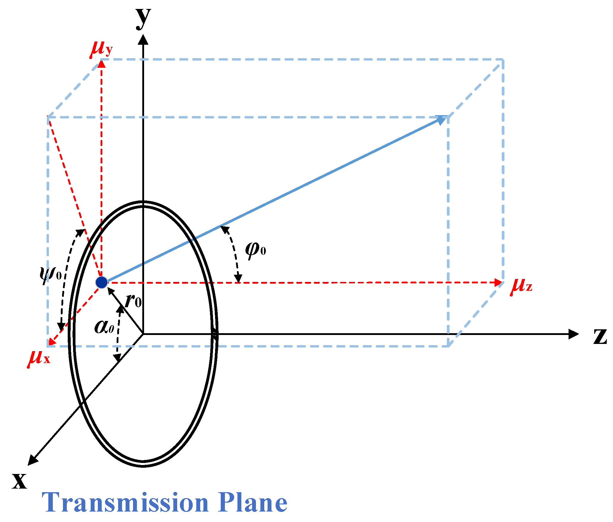
2.3.1. The Initial Parameters of Photon Packets

The Monte Carlo method is a stochastic simulation technique used to model the propagation of light in seawater. This method involves tracking the random propagation paths of numerous photons, thereby facilitating statistical analysis and calculation. In this approach, the light source is modeled as a collection of photon packets, each characterized by specific distribution properties. The simulation process is guided by the optical and water quality parameters pertinent to the communication system. The photon scattering angle, determined by the volume scattering phase function, plays a crucial role in this process. By tracking the trajectory of each photon, the method enables a detailed analysis of their motion paths. Ultimately, this simulation allows for the accumulation and analysis of data regarding the number of photons received and their distribution characteristics. Such comprehensive data are crucial for understanding and optimizing underwater communication systems.

In the Monte Carlo simulation, the initial parameters of a photon are defined by its initial coordinates $(x_0, y_0, z_0)$ on the Transmission Plane and the directional components $({\mu }_{0x},{ \mu }_{0y},{ \mu }_{0z})$ of the photon’s direction vector along the x, y, and z axes, respectively. These directional components, commonly referred to as Direction Cosines, determine the photon’s propagation direction, while the coordinates indicate its current position. As illustrated in Figure 4, we assume that the photon packet travels along the z-axis and lies on the Transmission Plane.

In the depicted setup, the Transmission Plane is situated within the x–y plane. The solid blue arrow in Figure 4 represents the initial direction vector of the photon packet. Additionally, the dashed blue rectangle illustrates the initial photon motion coordinate system, which undergoes changes with each photon scattering event. It is important to note that, despite the dynamic nature of the photon motion coordinate system, the coordinate system established by the transmitter and receiver remains constant. In other words, the x, y, and z axes, as shown in Figure 4, are fixed. This distinction between the changing photon motion coordinate system and the static system set by the transmitter and receiver is crucial for understanding the dynamics of photon movement and scattering in the simulation.

Here, ($r_0$, ${\alpha }_0$) is the polar coordinate for the initial photon position in the Transmission plane, the distance between the photon packet’s current position, and the center of the light source is denoted as $r_0$. Additionally, the initial azimuth angle (${\mathrm{\psi }}_0$) and elevation angle (${\phi }_0$) of the photon are specified. The photon’s initial weight is set to $\omega =1$.

The initial coordinates of the photon $(x_0,{ y}_0,{ z}_0)$ and the Direction Cosines $({\mu }_{0x},{ \mu }_{0y},{ \mu }_{0z})$ are derived using trigonometric functions, as shown in Equations (5) and (6).

$$\left\{\begin{array}{c}{x}_0=r_{0}cos{\alpha }_0\\ y_0=r_{0}sin{\alpha }_0\\ z_0=0\end{array}\right.$$

(5)

$$\left\{\begin{array}{c}{\mu }_{0x}=sin{\phi }_{0}cos{\mathrm{\psi }}_0\\ {\mu }_{0y}=sin{\phi }_{0}sin{\mathrm{\psi }}_0\\ {\mu }_{0z}=cos{\phi }_0\end{array}\right.$$

(6)

In the Monte Carlo simulation process, the beam of the light source does not necessarily have to be azimuthally isotropic. The initial angle and the position for a photon packet should always be random, irrespective of the symmetrical nature of the beam. ${\alpha }_0$ and ${\mathrm{\psi }}_0$ can be randomly determined, this random selection is guided by Equation (7), where $R$ represents a random value within the normalized interval [0, 1]. This method ensures that the angles are uniformly distributed, aligning with the radial symmetry of the light source and beam configuration.

$$\left\{\begin{array}{c}{\alpha }_0=2\pi R\\ {\mathrm{\psi }}_0=2\pi R\end{array}\right.$$

(7)

The energy distribution of the laser beam in the simulation follows Gaussian distribution characteristics. This distribution is crucial for determining the radius $r_0$ on the Transmission Plane, which represents the distance between a given photon and the center of the light source. The calculation of $r_0$ is based on the Gaussian distribution, as outlined in Equation (8). In this equation, $w_0$ represents the waist radius of the laser beam, and $R$ is a random value drawn from the normalized interval [0, 1].

$$r_0=w_0\sqrt{-ln(1-R)}$$

(8)

The initial elevation angle ${\phi }_0$ of each photon is derived based on the initial divergence half-angle (${\theta }_{div}$) of the beam, the beam waist radius ($w_0$), and the radius ($r_0$) on the Transmission Plane. The specific relationship among these parameters is articulated in Equation (9) [15]. This equation ensures that the elevation angle of each photon is accurately aligned with the beam’s divergence characteristics.

$${\phi }_0=\frac{r_0{\theta }_{div}}{w_0}$$

(9)

The Equations (5)–(9) discussed previously demonstrate that the initial elevation angle, initial azimuth angle, and initial position of each photon in the Monte Carlo simulation are determined through random calculations. This randomization process is crucial for accurately simulating the inherently stochastic nature of photon behavior in harbor water.

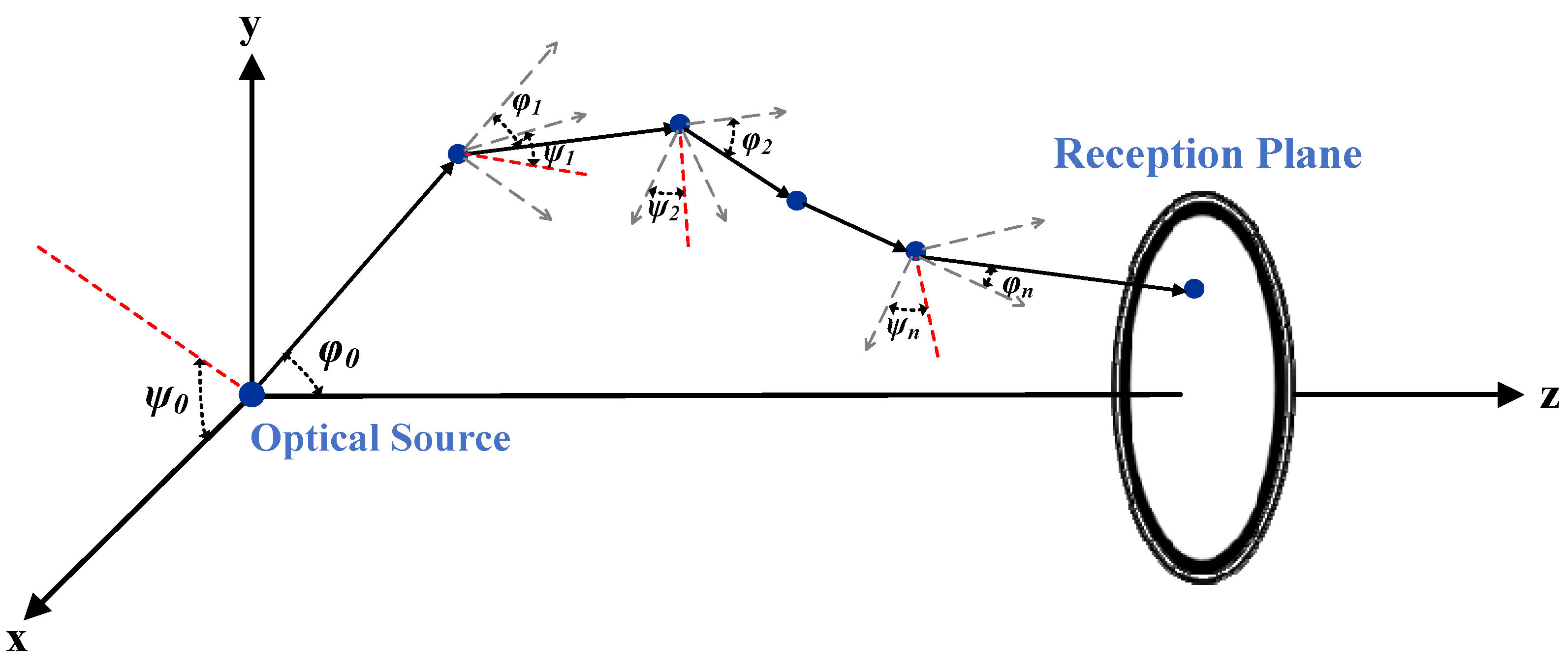
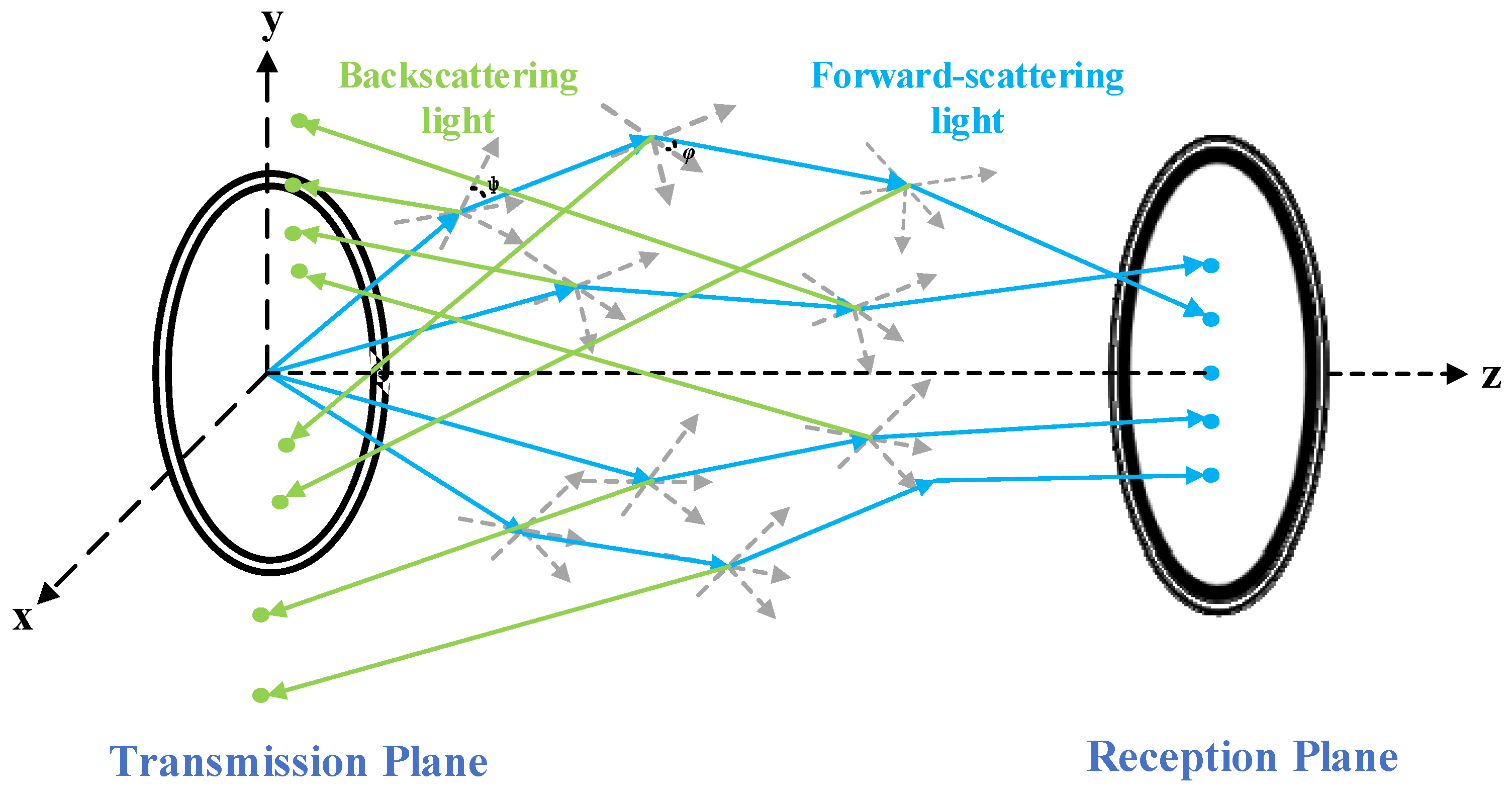
2.3.2. The Movement and Scattering of the Photon

The Monte Carlo simulation process is comprehensively illustrated in Figure 5, which presents a detailed flowchart. A critical aspect of this simulation involves determining the random scattering path length ($L$), scattering angle ($\phi$), and azimuth angle ($\mathrm{\psi }$) for each photon during its movement through the simulated environment. The scattering path length $L$ is defined as the distance a photon travels between two consecutive scattering events. This length is crucial as it influences the photon’s trajectory and the overall simulation accuracy.

The scattering angle $\phi$ of the photon after each collision with the particles in harbor water is randomly calculated by the scattering phase function $\tilde{\beta }\left(\phi \right)$ in Equation (3). The new azimuth angle $\mathrm{\psi }$ is calculated randomly by the equation $\mathrm{\psi }=2\pi R$, and the random scattering path length $L$ is calculated randomly by the Equation (11). $R$ is also a random value drawn from the normalized interval [0, 1] in the calculation of the propagation length $L$ and azimuth angle $\mathrm{\psi }$. The photon’s weight is updated by the equation ${\omega }_n={\omega }_{n-1}\ast {\omega }_0$, where, $n$ represents the $n$-th photon scattering event. Two critical steps in the simulation are the block «Calculate Euclidian distance to Rx plane» and «Calculate y, z intersection point», which mean that if the Euclidian distance between the photon’s position and the Reception Plane’s center is smaller than the received aperture, and if the angle between the y axis of the photon moving coordinate system and the z axis of the coordinate system built by the transceiver terminal is smaller than the Received FOV, the photon is thought to be able to reach the Reception Plane, then record the corresponding scattering angle meanwhile. Russian roulette is also introduced, and its function is: when the photon’s weight ${\omega }_n$ is greater than the setting threshold, the photon scattering process continues to be tracked, and the subsequent flow and algorithm are consistent with the previous. When the photon’s weight ${\omega }_n$ is less than the setting threshold, the photon is considered to have been annihilated completely.

During the simulation, the Transmission Plane and the Reception Plane are parallel to each other, and the fixed coordinate axis z is always perpendicular to the Reception Plane, so the orientation of the receiver can be confirmed. The position of the receiver can be confirmed by the setting values of the AL during simulation.

Equation (10) then provides further detail on how this angle is determined, with ${\phi }^{\prime }$ representing the specific scattering angle chosen during a scattering event, and $R$ still represents a random value drawn from the normalized interval [0, 1]. These steps are integral to accurately simulating the random paths of photons through water, crucial for understanding light behavior in underwater communication channels.

$${\int }_0^{{\phi }^{\prime }}\tilde{\beta }\left(\phi ,\mathsf{\lambda }\right)\mathit{sin}\left(\phi \right)d\phi =R$$

(10)

When the random scattering path length $L$, scattering angle $\phi$ and azimuth angle $\mathrm{\psi }$ of the photon are confirmed, the position of the photon can be updated as $\left[x^{\prime },y^{\prime },z^{\prime }\right]$ in Equation (12), where ${\mu }_x$, ${\mu }_y$, and ${\mu }_z$ are the Direction Cosine of the photon in the current state, the scattering path length $L$ is selected randomly in Equation (11) [50,51], where $b$ is the scattering coefficient, and $R$ is a random value drawn from the normalized interval [0, 1].

$$L=-\mathit{ln}\left(R\right)/b$$

(11)

$$\left\{\begin{array}{c}{x}^{\prime }=x_0+L{\mu }_x\\ y^{\prime }=y_0+L{\mu }_y\\ z^{\prime }=z_0+L{\mu }_z\end{array}\right.$$

(12)

The photon packet’s new weight, ${\omega }_n,$ is obtained further after $n$ scattering events. ${\omega }_0$ is the ratio of the scattering coefficient $b\left(\lambda \right)$ to the attenuation coefficient $c\left(\lambda \right)$ known as the albedo, $0{<\omega }_0<1$. The initial weight $\omega =1$, so with the increase of $n$, its weight ${\omega }_n$ decays gradually, as shown in Equation (13) and Figure 6.

$${\omega }_n=\omega \ast {\left({\omega }_0\right)}^n={\left({\omega }_0\right)}^n$$

(13)

When the photon’s new position is determined and is still in front of the Reception Plane, it is still possible to be absorbed by the receiver. The scattering angle and azimuth angle of the photon are reselected to obtain the new Direction Cosine $[{\mu }_x^{\prime }, {\mu }_y^{\prime }, {\mu }_z^{\prime }]$ in Equation (14), where ${\mu }_s=cos{\phi }^{\prime }$, ${\phi }^{\prime }$ and ${\mathrm{\psi }}^{\prime }$ are the new scattering angle and azimuth angle of the photon, respectively.

${\mu }_z$ is one of the moving photon’s Direction Cosine, and its square ${\mu }_z^2$ must be more than 0. In addition, in the Equation (14), to ensure that $\sqrt{1-{\mu }_z^2}$ is meaningful and rational, $1-{\mu }_z^2$ must be greater than 0, namely, $0<{\mu }_z^2<1$.

$$\left[\begin{array}{c}{\mu }_x^{\prime }\\ {\mu }_y^{\prime }\\ {\mu }_z^{\prime }\end{array}\right]=\left[\begin{array}{ccc}\raisebox{1ex}{${\mu }_x{\mu }_z$}\!\left/ \!\raisebox{-1ex}{$\sqrt{1-{\mu }_z^2}$}\right.& \raisebox{1ex}{$-{\mu }_y$}\!\left/ \!\raisebox{-1ex}{$\sqrt{1-{\mu }_z^2}$}\right.& {\mu }_x\\ \raisebox{1ex}{${\mu }_y{\mu }_z$}\!\left/ \!\raisebox{-1ex}{$\sqrt{1-{\mu }_z^2}$}\right.& \raisebox{1ex}{${\mu }_x$}\!\left/ \!\raisebox{-1ex}{$\sqrt{1-{\mu }_z^2}$}\right.& {\mu }_y\\ -\sqrt{1-{\mu }_z^2}& 0& {\mu }_z\end{array}\right]\left[\begin{array}{c}\sqrt{1-{\mu }_s^2}cos{\mathrm{\psi }}^{\prime }\\ \sqrt{1-{\mu }_s^2}sin{\mathrm{\psi }}^{\prime }\\ {\mu }_s\end{array}\right],{\mu }_z^2<1$$

(14)

2.3.3. Termination of Photon Motion or Reception of Photon

In the simulation, the termination of a photon’s motion is defined under two specific conditions. First, a photon is considered absorbed by the particles in the harbor water if its weight decreases to a threshold of 10⁻⁶ or less. The choice of the minimum threshold will affect the calculation time of the simulation, and is also related to the link loss needed to add into the simulation, that is, the AL. The larger the link loss to be added, the smaller the threshold. Second, the photon’s transmission is deemed to have ended once it reaches the receiver’s photosensitive surface.

Throughout the photon tracking process, key attributes of each photon are recorded, including its position, received angle, weight, and propagation distance. A photon is classified as ‘Received’ if it falls within the bounds of the receiver’s photosensitive surface and if its received angle is within the specified FOV. If either of these conditions is not met, the photon is considered ‘not Received’, and its tracking is discontinued.

This methodical approach allows for precise determination of photon reception, facilitating an accurate assessment of the efficiency and effectiveness of the UWOC system in various harbor water conditions.

3. The Simulation Results and Discussion

In this paper, we primarily investigate the characteristics of UWOC with varying communication distances in four distinct types of harbor water. To facilitate this study, certain parameters of the transmitter and receiver are predetermined and held constant, with the main variable parameters being the transmitted full divergence angle, the received aperture, and the received FOV.

The transmitted full divergence angle significantly impacts the initial scattering angle ${\phi }_0$ of photon, as described in Equation (9), and the corresponding beam waist radius influences the initial position of photons, as indicated by Equations (5) and (8). These factors dictate the varied paths photons traverse, thereby affecting the number and time of photons reaching the Reception Plane. Consequently, this variation directly influences the normalized power loss and time delay spread. The received aperture and FOV determine the receiver’s capability to collect photons, with the different number of photons received resulting in variations in received optical power. Moreover, the disparate photon counts lead to discrepancies in the statistical timing of photons arriving at the Reception Plane, ultimately affecting both normalized power loss and time delay spread.

Reflecting the focus of our research, we have established a set of initial fixed parameters for use in our simulation model. These parameters, detailed in

Table 2. Initial fixed parameters utilized in the simulation.

Wavelength	Transmitted Photon Number	Single Photon Energy	Transmitted Light Energy
532 nm	1013	3.74 × 10−19 J	3.74 × 10−6 J

, include the laser wavelength, the number of photons transmitted, the single photon energy, and the total transmitted light energy.

This approach ensures a consistent baseline for analyzing the impact of the aforementioned variable parameters on the performance of UWOC systems in different harbor water conditions.

The specific settings for the transmitted full divergence angle, as outlined in

Table 3. Setting values for the transmitted full divergence angle, transmitted beam waist diameter, received aperture and received FOV.

Transmitted full divergence angle (2${\mathit{\theta }}_{\mathit{d}\mathit{i}\mathit{v}}$)	0.5 mrad		5 mrad		10 mrad		100 mrad
Transmitted beam waist diameter (2${\mathit{w}}_0$)	1.4 × 10−3 m		1.35 × 10−4 m		6.77 × 10−5 m		6.77 × 10−6 m
Received aperture	25 mm		50 mm	100 mm		200 mm	400 mm
Received FOV	$\frac{\pi }{90}$ rad	$\frac{\pi }{30}$ rad	$\frac{\pi }{22.5}$ rad	$\frac{\pi }{15}$ rad	$\frac{\pi }{7.5}$ rad	$\frac{\pi }{2}$ rad	$\frac{\pi }{1.5}$ rad	$\pi$ rad

, include values of 0.5 mrad, 5 mrad, 10 mrad, and 100 mrad. The Transmitted half divergence angle ${(\theta }_{div})$ of the Gaussian beam is defined as when the transmission distance $z\to \infty$, the angle between the position with 1/e times the center maximum amplitude of the Far-field spot with z axis, as shown in the Figure 7 below. The Transmitted full divergence angle is $2{\theta }_{div}$.

The Far-field spot of the Gaussian beam is the spot determined by the position with 1/e times the center maximum amplitude, the spot radius $w\left(z\right)$ in the propagation direction is shown in Equation (15), where $w_0$ is the beam waist radius.

$$w\left(z\right)=w_0\sqrt{1+{\left(\frac{\lambda z}{\pi w_0^2}\right)}^2}$$

(15)

So, the Transmitted full divergence angle $2{\theta }_{div}$ can be derived:

$$2{\theta }_{div}=2\underset{z\to \infty }{\mathit{lim}}\frac{w\left(z\right)}{z}=\frac{2\lambda }{\pi w_0}$$

(16)

Corresponding to these full divergence angles, the Transmitted beam waist diameter ($2w_0$) for each setting is calculated using Equation (16). In the analysis of how these varying transmitted full divergence angles affect the communication system, both the received aperture and the received FOV are held constant. They are fixed at 200 mm for the received aperture and $\pi /2$ rad for the received FOV. This methodical approach allows for a focused investigation into the impact of the transmitted full divergence angle on UWOC system performance, ensuring that other variables do not confound the results.

The specific settings for the received FOV and aperture are also detailed in Table 3. The received aperture sizes are set at 25 mm, 50 mm, 100 mm, 200 mm, and 400 mm. The values for the received FOV are varied and include $\pi /90$ rad, $\pi /30$ rad, $\pi /22.5$ rad, $\pi /15$ rad, $\pi /7.5$ rad, $\pi /2$ rad, $\pi /1.5$ rad, and $\pi$ rad. In the analysis that focuses on the impact of these variable received aperture and FOV on the communication system, the transmitted full divergence angle is consistently fixed at 0.5 mrad. This approach enables a targeted examination of how changes in the received aperture and FOV affect the performance of the UWOC system, isolating these variables to understand their specific contributions.

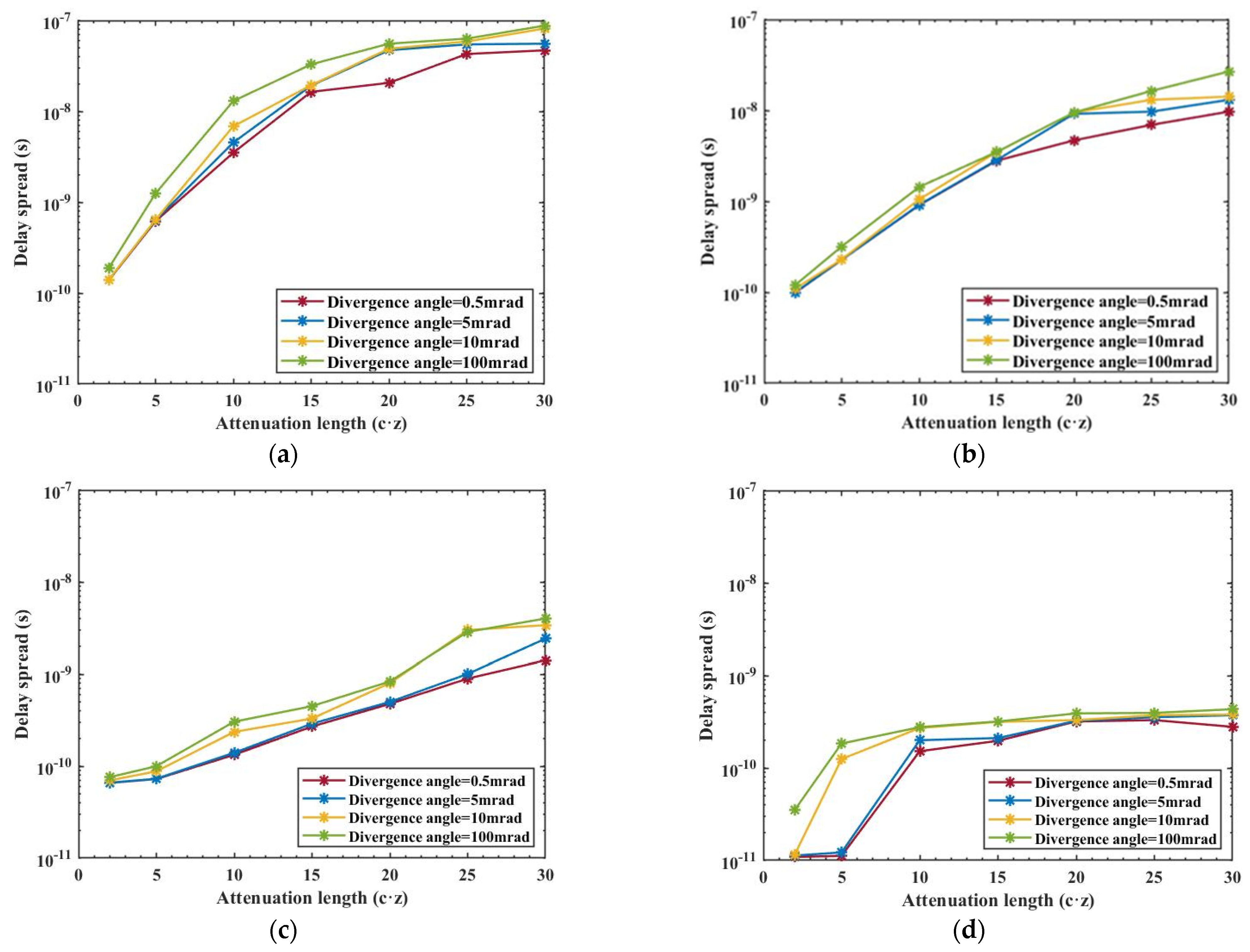
3.1. Analytical Examination of the Full Divergence Angle in Transmission

In this study, we analyze the variation characteristics of laser power in relation to both the attenuation length and the divergence angle. Figure 8 illustrates the normalized power loss received as a function of the AL and the transmitted full divergence angle. The AL is defined as the product of the attenuation coefficient $c\left(\lambda \right)$ and the communication distance $z$, expressed mathematically as AL $=c\left(\lambda \right)\times z$.

Simulation results indicate a consistent trend across all four types of harbor water: as AL increases, there is a corresponding increase in the attenuation loss of received power. Notably, the attenuation of received optical power initially occurs at a rapid rate and then stabilizes. This pattern is attributed to the gradual divergence of the light beam, which leads to a swift attenuation of light energy over a short distance. As the transmission distance extends, the light beam enters a state of full scattering. In this phase, the proportion of energy attenuation due to light scattering gradually diminishes, making absorption the predominant factor affecting light transmission. This trend is particularly evident in Figure 8a, highlighting the dynamic interplay between scattering and absorption in determining the attenuation characteristics of UWOC. Furthermore, our analysis reveals that a larger transmitted full divergence angle correlates with greater normalized optical power attenuation loss. This trend holds consistently across the four types of harbor water.

The normalized power loss of four harbor water in Figure 8 is different based on the same AL, which is inconsistent with the traditional Beer–Lambert law. This indicates that the Beer–Lambert law is completely inapplicable in harbor water due to the extreme scattering property, which is also confirmed by the reference [52], and the common approach in many studies of directly deriving communication distance by dividing the attenuation coefficients of two different water types proves to be inapplicable in the context of harbor water. The Monte Carlo algorithm is the valid solution for these highly scattering communication scenarios. This finding underscores the complexity of the relationship between water quality, communication distance, and light attenuation in UWOC, challenging assumptions that may hold true in other types of aquatic environments.

In addition, with the same AL and divergence angle, it is shown that the normalized power loss is decreasing (↓) as the water quality deteriorates ($c$↑) and the communication distance decreases ($z$↓) in Figure 8. It can be concluded that in harbor water, the influence of communication distance on normalized power loss is more significant; in other words, the impact of water quality is overshadowed by the sheer magnitude of communication distance $z$-induced losses. This phenomenon is attributed to that intensified photons scattering in more deteriorating water might increase the diversity of photons reaching the Reception Plane, this diversification may offset some of the power loss, leading to a reduction in normalized power loss.

Our findings also indicate that the differences in normalized power loss among smaller divergence angles, specifically 0.5 mrad, 5 mrad, and 10 mrad, are relatively minor compared to a larger angle like 100 mrad. The primary reason for this is that a smaller transmitted full divergence angle confines the light spot within a more limited range. This confinement results in reduced geometric loss and diminishes the likelihood of photons being scattered by particles in the water. Consequently, a smaller divergence angle ensures that a higher number of photons can reach the photosensitive surface of the receiver and be effectively absorbed. This observation underscores the significance of divergence angle control in minimizing power loss in UWOC, particularly in environments with scattering particles.

Differences in the simulation results depicted in Figure 8a–d have been calculated, for example with a full divergence angle of 100 mrad and an AL of 30, the power loss of Harbor II, III, and IV are found to be 14.00 dB, 31.59 dB, and 41.59 dB lower, respectively, than that of Harbor I. So, the normalized power loss of Harbor II, III, and IV is 3.98%, 0.069%, and 0.0069% times that of the Harbor I.

In our next analysis, we examine the time delay spread in relation to both the AL and the transmitted full divergence angle across the four types of harbor water, as depicted in Figure 9. We observe that under identical harbor water condition, the time delay spread increases with both the increase in AL and the transmitted full divergence angle. Conversely, for a given AL and divergence angle, the time delay spread decreases as the quality of harbor water deteriorates. This trend mirrors the observed behavior in normalized power loss, indicating that the influence of communication distance $z$ on time delay spread is more significant than water quality; in other words, the impact of water quality is overshadowed by the substantial losses induced by the communication distance $z$. We consider that increase in scattering events may boost the incidence of forward scattering, which could reduce the variability in the paths photons travel to the Reception Plane, thus resulting in a decrease in time delay spread.

Additionally, Figure 9d highlights a specific scenario where the AL ranges from 2–5 and the transmitted full divergence angle is between 0.5 mrad and 5 mrad. In this case, the time delay spread is notably low, ranging only from 1.09 × 10⁻¹¹–1.22 × 10⁻¹¹ s. This minimal spread can be attributed to the relatively short transmission distance, approximately 0.45 m to 1.14 m, which is insufficient to contribute significantly to the time delay spread. This finding emphasizes the importance of considering both the transmission distance and beam divergence characteristics when assessing the time delay in UWOC.

The results in Figure 9a–d have been also numerically analyzed, the time delay spread of Harbor II, III, and IV is 30.56%, 9.67%, and 0.49% times that of the Harbor I, when full divergence angle is 100 mrad, AL is 30. The differences of normalized power loss are much smaller than that of time delay spread. This indicates that the influence of absorption and scattering on power loss is much greater than that of scattering on time delay spread.

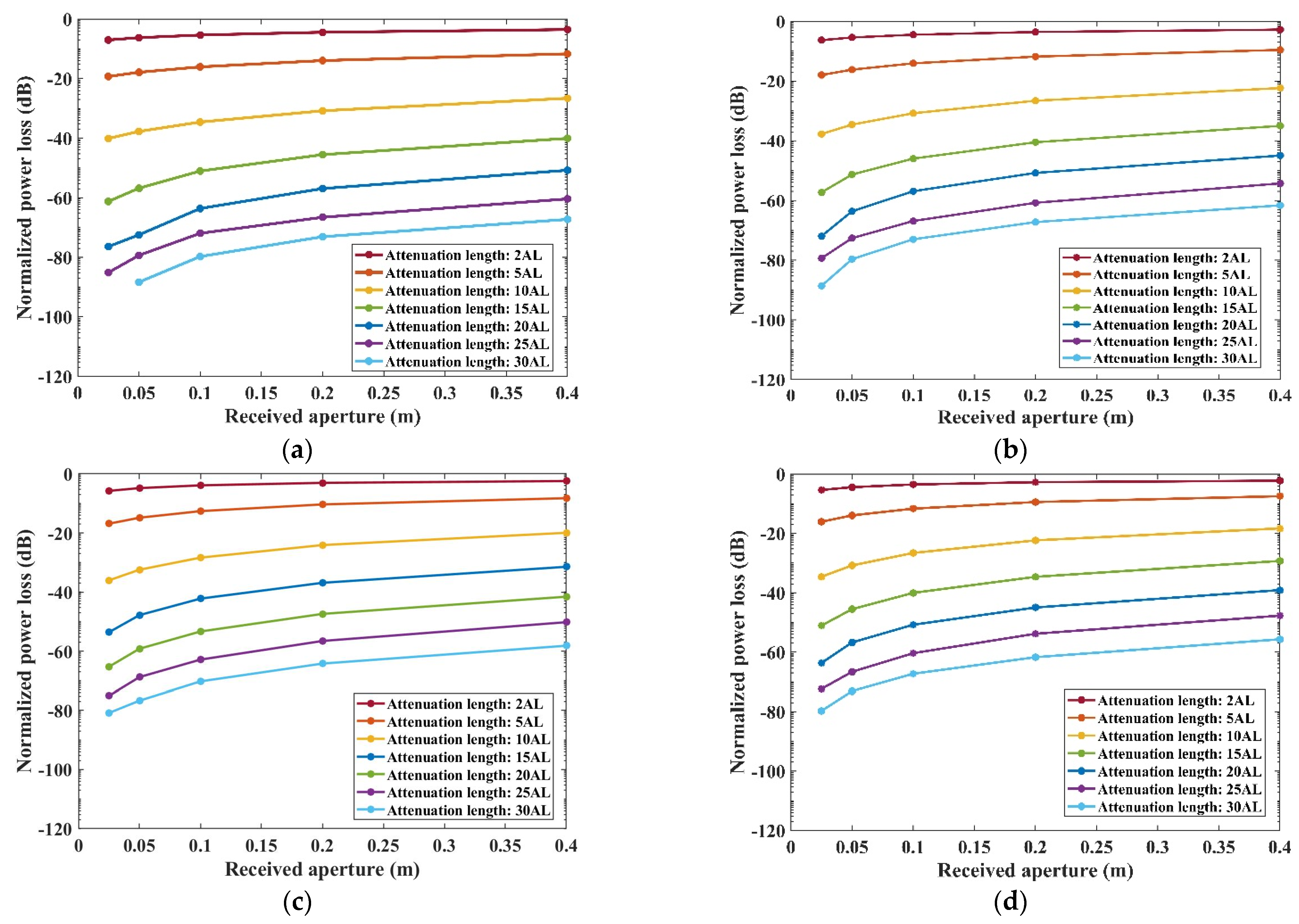
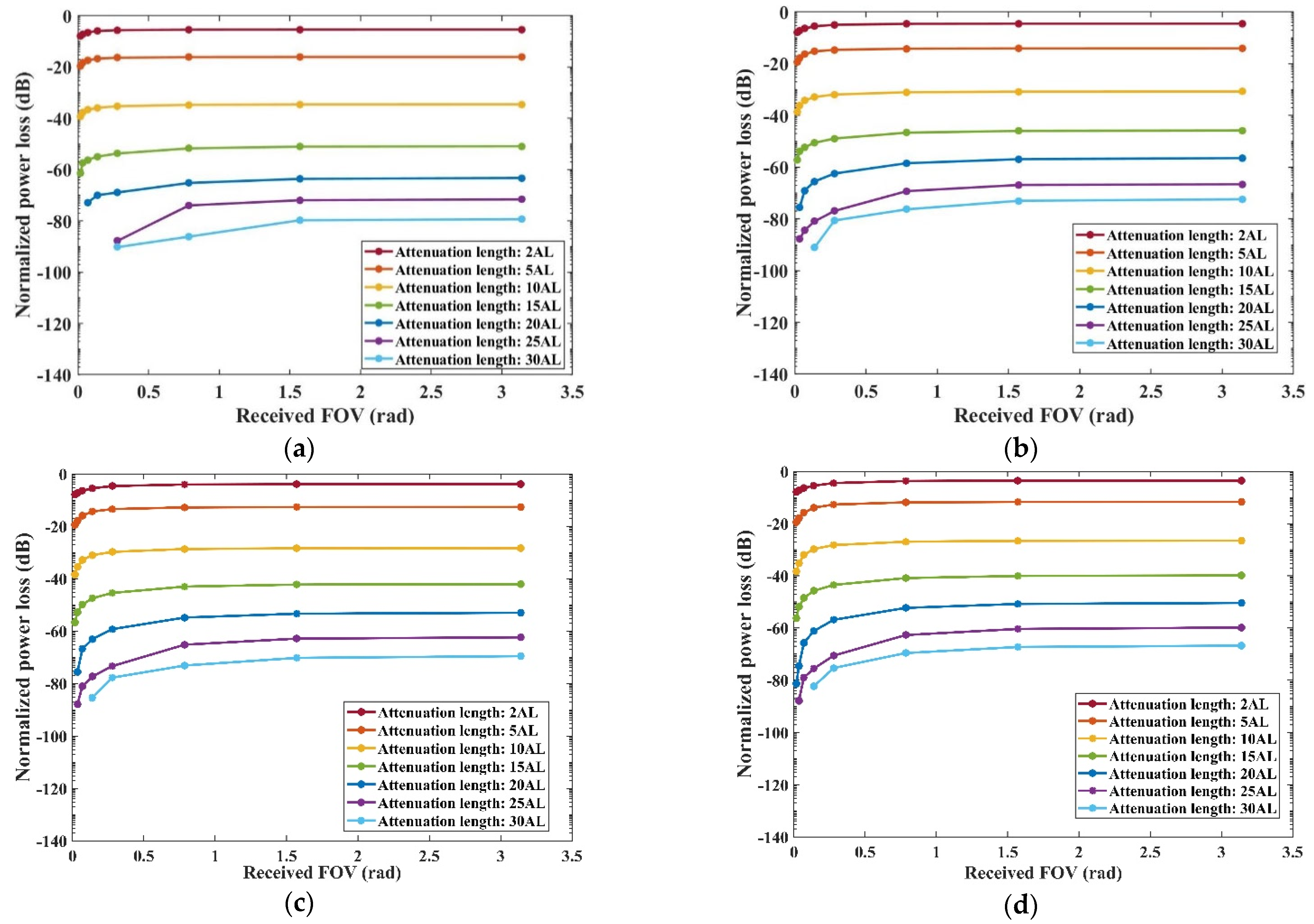
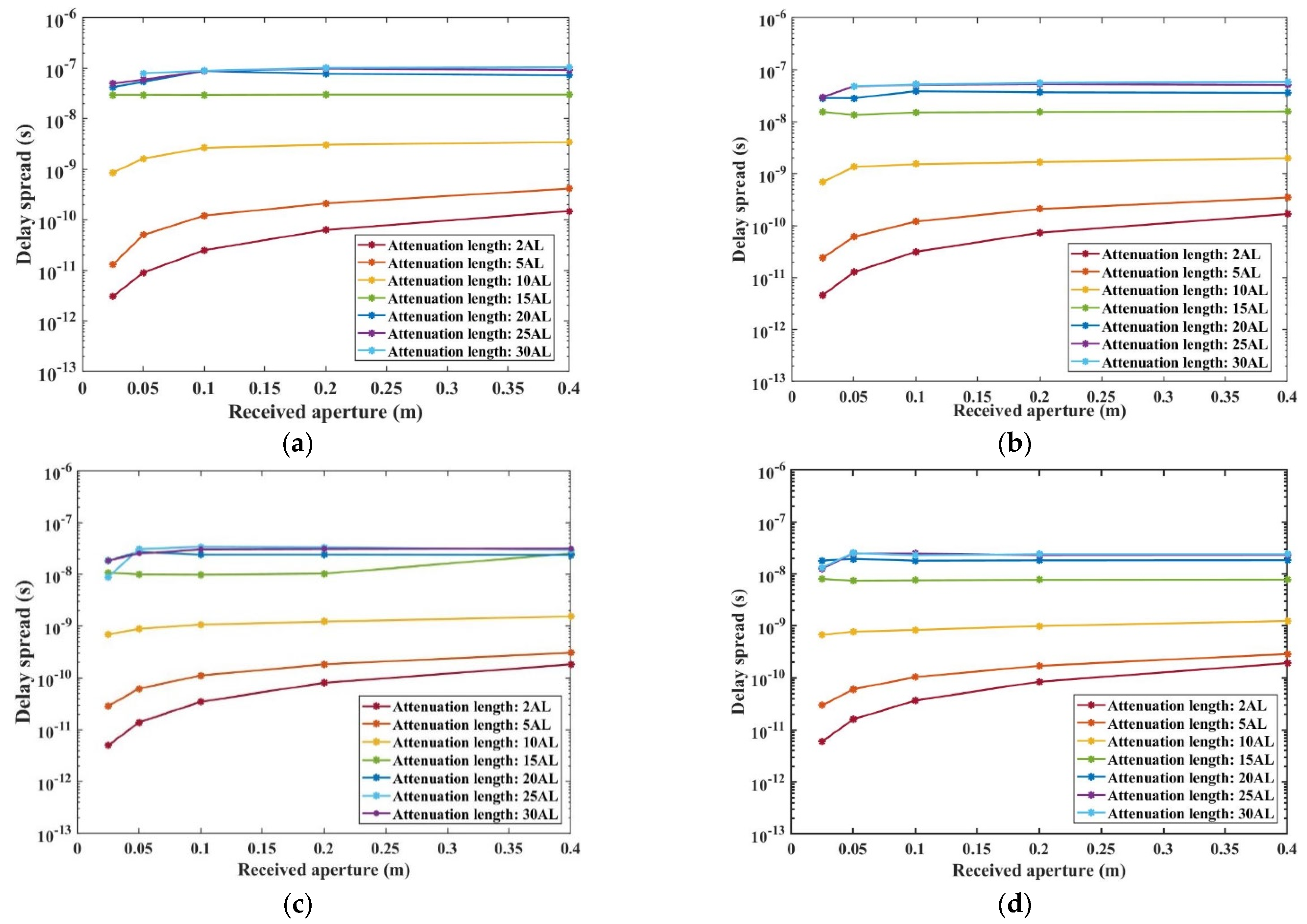
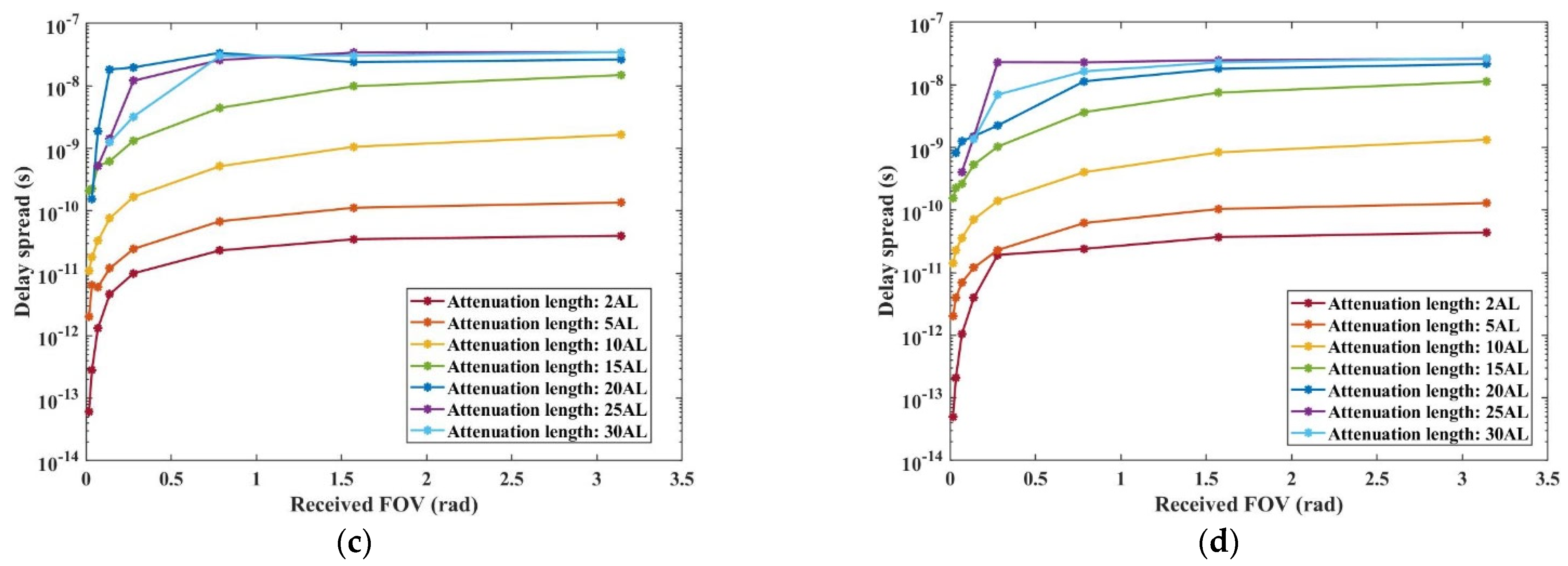
3.2. Analytical Evaluation of the Received Aperture and FOV

The study also examines how normalized power loss correlates with AL and the size of the Received aperture at the receiver’s end, as illustrated in Figure 10. Our simulations reveal a consistent relationship between these variables across the four types of harbor water. Notably, as the size of the received aperture increases, the normalized power loss decreases. However, the rate of this decline slows and eventually stabilizes. This trend is attributed to the fact that a larger received aperture can capture more scattered photons, thus enhancing the absorption efficiency of the receiver.

Additionally, it is evident that larger AL values correspond to greater normalized power losses. This relationship underscores the significant impact of communication distance and beam attenuation characteristics on the efficiency of photon reception in UWOC systems.

The relationship between normalized power loss, AL, and received FOV at the receiving end is further explored in Figure 11, focusing on the four types of harbor water. Simulation results indicate that the trends in normalized power loss correspond closely with both AL and the received FOV across these water types. In scenarios where the received FOV is relatively small (<0.2793 rad), there is a noticeable decrease in normalized power loss as the FOV increases. This decrease is attributed to the fact that a larger FOV allows more photons, particularly those deviating from the optical axis, to become On-target photons and be absorbed by the receiver. However, as the received FOV continues to expand beyond this point, the impact on normalized power loss diminishes. This plateau in the effect is due to the large FOV eventually encompassing almost the entire peak intensity region of the Gaussian beam on the Reception Plane. Consequently, further increases in FOV do not significantly affect the proportion of photons captured, thereby stabilizing the normalized power loss.

In our final analysis, we examine the time delay spread at the receiving end in relation to AL, the size of the received aperture, and the received FOV across the four types of harbor water. This analysis is illustrated in Figure 12 and Figure 13, and our findings indicate that, under constant harbor water conditions, the time delay spread increases with the rising AL. In the range of shorter ALs (2–10 AL), as shown in Figure 12, the time delay spread enlarges with an increase in the size of the received aperture. This trend is attributed to the fact that a larger aperture increases the likelihood of capturing multiple-scattered photons. However, in scenarios involving larger ALs (15–30 AL), the time delay spread exhibits minimal variation in response to changes in the received aperture size, remaining within the range of 1.05 × 10⁻⁷ s to 7.39 × 10⁻⁹ s. The primary reason for this is that at longer communication distances, most scattered photons become Off-target photons due to multiple scatterings, and thus they are unlikely to be absorbed by the receiver. Consequently, in the range of 15–30 AL, the time delay spread remains relatively constant.

In the case of a small received FOV (less than 0.8 rad), as depicted in Figure 13, there is a noticeable increase in the time delay spread as the FOV gradually expands. This pattern arises because a larger received FOV enhances the receiver’s capability to capture a greater number of multiple-scattered photons. As a result, the time delay spread grows with the increasing FOV.

However, beyond a certain point, the rate of increase in time delay spread significantly slows down. This slowdown occurs because a larger FOV eventually encompasses most of the multiple-scattered photons within the Reception Plane. Therefore, further increases in the FOV do not substantially add to the number of photons captured, leading to only marginal changes in the time delay spread. This finding illustrates the intricate balance between FOV and the efficiency of photon capture in determining the time delay characteristics of UWOC systems.

Lastly, the simulation results and theoretical analysis collectively suggest that increasing the received aperture and FOV, particularly over longer communication distance, make little contribution to reduce the normalized power loss and mitigate the time delay spread, thus not significantly enhancing communication quality. The primary reason is that, although a larger received aperture and FOV can capture more scattered photons, beyond a certain threshold, these parameters expand to cover nearly the entire peak intensity region of the Gaussian beam or most of the multiple-scattered photons on the Reception Plane. Based on these findings and the fixed transmitted full divergence angle at 0.5 mrad, the most suitable received FOV range is about 1–3.2 rad, and the most ideal received aperture is about 0.15–0.4 m. The variations in normalized power loss, under threshold conditions, predominantly register at less than 2 dB. Furthermore, statistical analyses concerning the time delay spread, also under these threshold conditions, reveal that it generally maintains the same order of magnitude, given the same AL.

To gain a thorough understanding of the UWOC system’s performance in harbor water condition, we meticulously analyze the computational cost, a critical factor in our numerical simulations. The simulations are conducted on a computer equipped with an AMD Ryzen 9 5900X 12-core processor, operating at a main frequency of 3.7 GHz, and 64.0 GB of RAM, selected for its capability to efficiently process computationally intensive tasks. On average, the simulation process for each data point presented in Figure 8, Figure 9, Figure 10, Figure 11, Figure 12 and Figure 13 requires approximately 4.5 h.

4. Conclusions

This study has critically examined the UWOC within four distinct types of harbor water, employing the Monte Carlo method to simulate photon behavior and analyze key communication parameters. Our findings reveal that the Transmitted full divergence angle, received aperture, and FOV profoundly affect the UWOC system’s performance. According to the simulation results, the following three main conclusions can be drawn:

• Firstly, increased AL and divergence angle lead to higher received normalized power loss and time delay spread, the attenuation initially occurs at a rapid rate and then stabilizes, with these effects being more pronounced in clearer harbor water types.
• Secondly, this work reveals that the impact of communication distance on normalized power loss and time delay spread is more pronounced than that of water quality. This insight challenges that the common Beer–Lambert law no longer applies in harbor water. Communication distance, estimated by simply dividing the attenuation coefficients of different water types in many studies, is ineffective in harbor water contexts.
• Consequently, increasing the received aperture and FOV, particularly over longer communication distances, contributes minimally to reducing normalized power loss or mitigating time delay spread, thus not significantly enhancing communication quality. Based on the fixed transmitted full divergence angle, the most suitable received FOV range is about 1–3.2 rad, and the most ideal received aperture is about 0.15–0.4 m. This result holds substantial technical relevance for the engineering design of UWOC across a range of harbor water conditions.

It should be noted that this work simplifies the absorption and scattering models to facilitate analysis. We assume that the absorption and scattering characteristics of harbor water remain consistent throughout the photon’s travel path. However, real-world water bodies may display more complex scattering and absorption behaviors due to dynamic water movements. This simplification represents a minor limitation of our study.

All these insights and analysis results pave the way for more efficient design and optimization of UWOC systems, particularly in challenging harbor water environments, by providing a detailed understanding of the interplay between light scattering, absorption properties, and system configuration. Moreover, this study lays a technical and theoretical foundation that could facilitate the replication and expansion of our research into more turbid inland waters. Future research may develop more comprehensive models to accurately represent the diverse environmental conditions found in natural water bodies.

References

1. Li, J.; Yang, B.; Ye, D.; Wang, L.; Fu, K.; Piao, J.; Wang, Y. A real-time, full-duplex system for underwater wireless optical communication: Hardware structure and optical link mode. IEEE Access 2020, 8, 109372–109387. [Google Scholar] [CrossRef]
2. Yang, Y.; He, F.; Guo, Q.; Wang, M.; Zhang, J.; Duan, Z. Analysis of underwater wireless optical communication system performance. Appl. Opt. 2019, 58, 9808–9814. [Google Scholar] [CrossRef] [PubMed]
3. Zeng, Z. A Survey of Underwater Wireless Optical Communication. Master’s Thesis, University of British Columbia, Vancouver, BC, Canada, 2015. [Google Scholar]
4. Urick, R.J. Principles of Underwater Sound; Peninsula: Los Altos, CA, USA, 1983. [Google Scholar]
5. Xu, J. Underwater wireless optical communication: Why, what, and how? Chin. Opt. Lett. 2019, 17, 100007. [Google Scholar] [CrossRef]
6. Zhu, S.; Chen, X.; Liu, X.; Zhang, G.; Tian, P. Recent progress in and perspectives of underwater wireless optical communication. Prog. Quant. Electron. 2020, 73, 100274. [Google Scholar] [CrossRef]
7. Ali, M.F.; Jayakody, D.N.K.; Chursin, Y.A.; Affes, S.; Dmitry, S. Recent advances and future directions on underwater wireless communications. Arch. Comput. Methods Eng. 2020, 27, 1379–1412. [Google Scholar] [CrossRef]
8. Ma, L.; Zhou, S.; Qiao, G.; Liu, S.; Zhou, F. Superposition coding for downlink underwater acoustic OFDM. IEEE J. Ocean. Eng. 2016, 42, 175–187. [Google Scholar] [CrossRef]
9. Tian, P.; Liu, X.; Yi, S.; Huang, Y.; Zhang, S.; Zhou, X.; Hu, L.; Zheng, L.; Liu, R. High-speed underwater optical wireless communication using a blue GaN-based micro-LED. Opt. Express 2017, 25, 1193–1201. [Google Scholar] [CrossRef]
10. Kao, C.C.; Lin, Y.S.; Wu, G.D.; Huang, C.J. A comprehensive study on the internet of underwater things: Applications, challenges, and channel models. Sensors 2017, 17, 1477. [Google Scholar] [CrossRef]
11. Sun, X.; Kang, C.H.; Kong, M.; Alkhazragi, O.; Guo, Y.; Ouhssain, M.; Weng, Y.; Jones, B.H.; Ng, T.K.; Ooi, B.S. A review on practical considerations and solutions in underwater wireless optical communication. J. Light. Technol. 2020, 38, 421–431. [Google Scholar] [CrossRef]
12. Wang, J.; Yang, X.; Lv, W.; Yu, C.; Wu, J.; Zhao, M.; Qu, F.; Xu, Z.; Han, J.; Xu, J. Underwater wireless optical communication based on multi-pixel photon counter and OFDM modulation. Opt. Commun. 2019, 451, 181–185. [Google Scholar] [CrossRef]
13. Wang, L.; Qi, Z.; Liu, P.; Hu, F.; Li, J.; Wang, Y. Underwater wireless video communication using blue light. J. Light. Technol. 2023, 41, 5951–5957. [Google Scholar] [CrossRef]
14. Wei, W.; Zhang, X.; Rao, J.; Wang, W. Time domain dispersion of underwater optical wireless communication. Chin. Opt. Lett. 2011, 9, 030101. [Google Scholar] [CrossRef]
15. Li, J.; Luo, J.; Li, S.; Yuan, X. Centroid drift of laser beam propagation through a water surface with wave turbulence. Appl. Opt. 2020, 59, 6210–6217. [Google Scholar] [CrossRef]
16. Cox, W.C., Jr. Simulation, Modeling, and Design of Underwater Optical Communication Systems. Ph.D. Thesis, North Carolina State University, Raleigh, NC, USA, 2012. [Google Scholar]
17. Shen, C.; Guo, Y.; Oubei, H.M.; Ng, T.K.; Liu, G.; Park, K.H.; Ho, K.T.; Alouini, M.S.; Ooi, B.S. 20-meter underwater wireless optical communication link with 1.5 Gbps data rate. Opt. Express 2016, 24, 25502–25509. [Google Scholar] [CrossRef]
18. Sahu, S.K.; Shanmugam, P. A theoretical study on the impact of particle scattering on the channel characteristics of underwater optical communication system. Opt. Commun. 2018, 408, 3–14. [Google Scholar] [CrossRef]
19. Cochenour, B.M.; Mullen, L.J.; Laux, A.E. Characterization of the beam-spread function for underwater wireless optical communications links. IEEE J. Ocean. Eng. 2008, 33, 513–521. [Google Scholar] [CrossRef]
20. Ntziachristos, V. Going deeper than microscopy: The optical imaging frontier in biology. Nat. Methods 2010, 7, 603–614. [Google Scholar] [CrossRef] [PubMed]
21. Han, B.; Zhao, W.; Meng, J.; Zheng, Y.; Yang, Q. Study on the backscattering disturbance in duplex underwater wireless optical communication systems. Appl. Opt. 2018, 57, 8478–8486. [Google Scholar] [CrossRef] [PubMed]
22. Qin, J.; Fu, M.; Sun MZhen, C.; Ji, R.; Zheng, B. Simulation of beam characteristics in long-distance underwater optical communication. In Proceedings of the Global Oceans of the Conference, Singapore–US Gulf Coast, Biloxi, MS, USA, 5–30 October 2020; pp. 1–5. [Google Scholar]
23. Boluda-Ruiz, R.; Rico-Pinazo, P.; Castillo-Vázquez, B.; García-Zambrana, A.; Qaraqe, K. Impulse response modeling of underwater optical scattering channels for wireless communication. IEEE Photonic J. 2020, 12, 7904414. [Google Scholar] [CrossRef]
24. Bowen, A.D.; Jakuba, M.V.; Farr, N.E.; Ware, J.; Taylor, C.; Gomez-Ibanez, D.; Machado, C.R.; Pontbriand, C. An un-tethered ROV for routine access and intervention in the deep sea. In Proceedings of the 2013 Oceans-San Diego, San Diego, CA, USA, 23–27 September 2013; pp. 1–7. [Google Scholar]
25. Farr, N.E.; Ware, J.D.; Pontbriand, C.T.; Tivey, M.A. Demonstration of wireless data harvesting from a subsea node using a “ship of opportunity”. In Proceedings of the 2013 OCEANS-San Diego, San Diego, CA, USA, 23–27 September 2013; pp. 1–5. [Google Scholar]
26. Pontbriand, C.; Farr, N.; Hansen, J.; Kinsey, J.C.; Pelletier, L.-P.; Ware, J.; Fourie, D. Wireless data harvesting using the AUV Sentry and WHOI optical modem. In Proceedings of the OCEANS 2015-MTS/IEEE Washington, Washington, DC, USA, 19–22 October 2015; pp. 1–6. [Google Scholar]
27. Hubbard, W.A.; Bellmer, R.J. Biological and chemical composition of Boston Harbor, USA. Mar. Pollut. Bull. 1989, 20, 615–621. [Google Scholar] [CrossRef]
28. Ahmed, F.S.; Sensenich, B.A.; Gheni SA Znerdstrovic, D.; Dahhan, M.H. Bubble dynamics in 2D bubble column: Comparison between high-speed camera imaging analysis and 4-point optical probe. Chem. Eng. Commun. 2015, 202, 85–95. [Google Scholar] [CrossRef]
29. Li, J.; Ma, Y.; Zhou, Q.; Zhou, B.; Wang, H. Channel capacity study of underwater wireless optical communications links based on Monte Carlo simulation. J. Opt. 2011, 14, 015403. [Google Scholar] [CrossRef]
30. Kodama, T.; Sanusi, M.A.B.A.; Kobori, F.; Kimura, T.; Inoue, Y.; Jinno, M. Comprehensive analysis of time-domain hybrid PAM for data-rate and distance adaptive UWOC system. IEEE Access 2021, 9, 57064–57074. [Google Scholar] [CrossRef]
31. Gjerstad, K.I.; Stamnes, J.J.; Hamre, B.; Lotsberg, J.K.; Yan, B.; Stamnes, K. Monte Carlo and discrete-ordinate simulations of irradiances in the coupled atmosphere-ocean system. Appl. Opt. 2003, 42, 2609–2622. [Google Scholar] [CrossRef] [PubMed]
32. Gabriel, C.; Khalighi, M.A.; Bourennane, S.; Leon, P.; Rigaud, V. Channel modeling for underwater optical communication. In Proceedings of the IEEE GLOBECOM Workshops of the Conference, Houston, TX, USA, 5–9 December 2011; pp. 833–837. [Google Scholar]
33. Mobley, C.D. Light and Water: Radiative Transfer in Natural Waters; Academic Press: Boca Raton, FL, USA, 1994. [Google Scholar]
34. Tang, S.; Dong, Y.; Zhang, X. Impulse response modeling for underwater wireless optical communication links. IEEE Trans. Commun. 2013, 62, 226–234. [Google Scholar] [CrossRef]
35. Qadar, R.; Kasi, M.K.; Ayub, S.; Kakar, F.A. Monte Carlo–based channel estimation and performance evaluation for UWOC links under geometric losses. Int. J. Commun. Syst. 2018, 31, e3527. [Google Scholar] [CrossRef]
36. Zhang, J.; Kou, L.; Yang, Y.; He, F.; Duan, Z. Monte-Carlo-based optical wireless underwater channel modeling with oceanic turbulence. Opt. Commun. 2020, 475, 126214. [Google Scholar] [CrossRef]
37. Freda, W.; Piskozub, J. Improved method of Fournier-Forand marine phase function parameterization. Opt. Express 2007, 15, 12763–12768. [Google Scholar] [CrossRef]
38. Mobley, C.D.; Sundman, L.K.; Boss, E. Phase function effects on oceanic light fields. Appl. Opt. 2002, 41, 1035–1050. [Google Scholar] [CrossRef] [PubMed]
39. Gabriel, C.; Khalighi, M.A.; Bourennane, S.; Léon, P.; Rigaud, V. Monte-Carlo-based channel characterization for underwater optical communication systems. J. Opt. Commun. Netw. 2013, 5, 1–12. [Google Scholar] [CrossRef]
40. Jiang, R.; Sun, C.; Zhang, L.; Tang, X.; Wang, H.; Zhang, A. Deep learning aided signal detection for SPAD-based underwater optical wireless communications. IEEE Access 2020, 8, 20363–20374. [Google Scholar] [CrossRef]
41. Zhang, L.; Tang, X.; Sun, C.; Chen, Z.; Li, Z.; Wang, H.; Jiang, R.; Shi, W.; Zhang, A. Over 10 attenuation length gigabits per second underwater wireless optical communication using a silicon photomultiplier (SiPM) based receiver. Opt. Express 2020, 28, 24968–24980. [Google Scholar] [CrossRef]
42. Hu, S.; Mi, L.; Zhou, T.; Chen, W. 35.88 attenuation lengths and 3.32 bits/photon underwater optical wireless communication based on photon-counting receiver with 256-PPM. Opt. Express 2018, 26, 21685–21699. [Google Scholar] [CrossRef] [PubMed]
43. Mobley, C.D.; Gentili, B.; Gordon, H.R.; Jin, Z.; Kattawar, G.W.; Morel, A.; Reinersman, P.; Stamnes, K.; Stavn, R.H. Comparison of numerical models for computing underwater light fields. Appl. Opt. 1993, 32, 7484–7504. [Google Scholar] [CrossRef] [PubMed]
44. Sahu, S.K.; Shanmugam, P. A study on the effect of scattering properties of marine particles on underwater optical wireless communication channel characteristics. In Proceedings of the OCEANS of the Conference, Aberdeen, UK, 19–22 June 2017; pp. 1–7. [Google Scholar]
45. Cochenour, B.; Mullen, L.; Laux, A.; Curran, T. Effects of multiple scattering on the implementation of an underwater wireless optical communications link. In Proceedings of the OCEANS of the Conference, Boston, MA, USA, 18–21 September 2006; pp. 1–6. [Google Scholar]
46. Cox, W.; Muth, J. Simulating channel losses in an underwater optical communication system. J. Opt. Soc. Am. A 2014, 31, 920–934. [Google Scholar] [CrossRef] [PubMed]
47. Petzold, T.J. Volume Scattering Functions for Selected Ocean Waters; Scripps Institution of Oceanography, La Jolla Ca Visibility Lab: La Jolla, CA, USA, 1972. [Google Scholar]
48. Haltrin, V.I. One-parameter two-term Henyey-Greenstein phase function for light scattering in seawater. Appl. Opt. 2002, 41, 1022–1028. [Google Scholar] [CrossRef] [PubMed]
49. Fournier, G.R.; Forand, J.L. Analytic phase function for ocean water. In Proceedings of the Ocean Optics XII, Bergen, Norway, 26 October 1994; Volume 2258, pp. 194–201. [Google Scholar]
50. Jaruwatanadilok, S. Underwater wireless optical communication channel modeling and performance evaluation using vector radiative transfer theory. IEEE J. Sel. Area Commun. 2008, 26, 1620–1627. [Google Scholar] [CrossRef]
51. Ishimaru, A. Wave Propagation and Scattering in Random Media; Academic Press: New York, NY, USA, 1978. [Google Scholar]
52. Qadar, R.; Kasi, M.K.; Kakar, F.A. Monte Carlo based estimation and performance evaluation of temporal channel behavior of UWOC under multiple scattering. In Proceedings of the Oceans 2017-Anchorage, Anchorage, AK, USA, 18–21 September 2017; pp. 1–7. [Google Scholar]
Figure 1. Schematic diagram of On-target photon and Off-target photon in underwater channel.
Applsci 14 02493 g001
Figure 2. Photon motion coordinate systems in underwater channel.
Applsci 14 02493 g002
Figure 3. Forward-scattering light and Backscattering light in underwater channel.
Applsci 14 02493 g003
Figure 4. Schematic diagram of the initial position and orientation of the photon packet in the Transmission Plane.
Applsci 14 02493 g004
Figure 5. The flow chart of Monte Carlo simulation.
Applsci 14 02493 g005
Figure 6. Schematic illustration of changes in the photon packet’s weight.
Applsci 14 02493 g006
Figure 7. Schematic Transmitted divergence angle and Far-field light spot.
Applsci 14 02493 g007
Figure 8. Comparative analysis of normalized power loss relative to attenuation length and transmitted full divergence angle across four types of harbor water. (a) Harbor I; (b) Harbor II; (c) Harbor III; (d) Harbor IV.
Applsci 14 02493 g008
Figure 9. Variation of time delay spread in relation to attenuation length and transmitted full divergence angle across four types of harbor water. (a) Harbor I; (b) Harbor II; (c) Harbor III; (d) Harbor IV.
Applsci 14 02493 g009
Figure 10. Comparative analysis of normalized power loss relative to attenuation length and received aperture across four types of harbor water. (a) Harbor I; (b) Harbor II; (c) Harbor III; (d) Harbor IV.
Applsci 14 02493 g010
Figure 11. Analysis of normalized power loss in relation to attenuation length and received FOV across four types of harbor water. (a) Harbor I; (b) Harbor II; (c) Harbor III; (d) Harbor IV.
Applsci 14 02493 g011
Figure 12. Assessment of time delay spread relative to attenuation length and received aperture across four types of harbor water. (a) Harbor I; (b) Harbor II; (c) Harbor III; (d) Harbor IV.
Applsci 14 02493 g012
Figure 13. Analysis of time delay spread in relation to attenuation length and received FOV across four harbor water. (a) Harbor I; (b) Harbor II; (c) Harbor III; (d) Harbor IV.
Applsci 14 02493 g013aApplsci 14 02493 g013b