Analysis of Vehicle-Bridge Coupling Vibration Characteristics of Curved Girder Bridges

Abstract

When vehicles move on a bridge, the coupling effect between vehicles and bridges can affect driving safety and comfort, especially for curved bridges, therefore, choosing reasonable design parameters for curved bridges is crucial. In this article, a three-span curved continuous box-girder bridge was taken as the research object; the entire process of vehicle-bridge coupling vibration of highway curved girder bridges was conducted via numerical simulation and the vehicle-bridge coupling vibration analysis program Cmck 1.0 was developed. Then, the influence factors such as curvature radius, constraint mode, and vehicle characteristics on the vehicle-bridge coupling vibration of curved girder bridges were explored. The results showed that as the curvature radius increased, the dynamic response of the bridge offered a gradually decreasing trend and compared to the vertical dynamic response, the torsional response was more sensitive to the influence of the curvature radius. Different constraint methods significantly impacted the dynamic response of bridges, and the vertical and torsional dynamic responses of bridges under general constraint arrangement of straight bridges were increased compared to those under boundary conditions for curved beam bridges. As the axle load of the car decreases, the bridge mid-span vertical and torsional dynamic responses showed a decreasing trend. In contrast, the lateral dynamic response gradually increased.

1. Introduction

Compared to straight girder bridges, curved bridges exhibit significant “bending torsion coupling” due to the influence of curvature radius. Under load, the main girder generates a bending moment and torque, and the stress performance significantly differs to straight bridges [1,2,3]. At the same time, due to the vehicle’s movement along the curve, the reference coordinate system for establishing the car vibration equation is constantly changing. The setting of the bridge deck superelevation and the existence of centrifugal force make the radial vibration of the vehicle-bridge coupling system along the curve aspects that cannot be ignored. The coupling relationship of curved girder bridges is more complex than that of straight bridges [4,5]. There are many studies on the coupling vibration of vehicles and bridges in straight bridges [6,7]. The coupling effect is different as the vehicle moves. Cantero focused on vehicles moving on the bridge, investigated the changes in frequencies and modes of vibration of a vehicle-bridge system, and found that the varying vehicle positions had obvious influences on the modal properties of the vehicle and bridge [8]. Gara carried out a test and studied different load conditions of vehicles stationed over the bridge deck, and proposed that it is necessary to address the vehicle–bridge interaction model to capture the accurate bridge dynamic response [9]. Zakeri presented results suggesting that the eccentric vertical and lateral forces are the major excitation sources in vehicle-bridge coupling analysis [10], and relatively detailed research results were achieved. The method can be applied to analyzing curved beam bridges by “using straight instead of curved.” For example, Ma et al. [11] studied the coupling vibration characteristics and mechanisms of trains and small radius curved section groove beam bridges using the bisector method with a straight instead of curved arrangement, and with a curved railway simple-supported groove girder bridge located at a radius of 300m as the object. Guo et al. [12] used linear beam elements to approximate curved girder bridges and analyzed the impact of factors such as the number of lanes, deck smoothness, vehicle speed, and vehicle type on the impact coefficient. Liu et al. [13] adopted the processing method of replacing “curves” with “straight lines” to establish a two-axis seven-degree-of-freedom vehicle model. Zhou studied the level of road roughness and the relationship between road smoothness and wheel slip and jump, and found that higher levels of road roughness make it easier for jump and other phenomena to occur [14].

The “using straightness to replace curvature” analysis method has high computational efficiency. However, due to the lack of full consideration of the influence of curvature, it cannot accurately analyze the longitudinal and lateral vibration coupling mechanical behavior and bending-torsional coupling effect of curved girder bridges under the action of vehicles. However, compared to straight bridges, some curved girder bridges (such as road interchange ramps) have characteristics such as the inward inclination of the bridge surface, widening of the outer side, resulting in no vertical symmetry axis of the girder section, noticeable bending-torsional coupling effect, and centrifugal effect of the vehicles. The vehicle-bridge coupling vibration mechanism is complex, and more fundamental studies in this area and limited applications are needed [15].

This article utilized the vehicle-bridge coupling vibration analysis method for straight bridges, theoretically analyzed the vehicle-bridge coupling relationship for curved girder bridges, and used curved girder units to simulate curved girder bridges. Combined with the vehicle dynamic analysis model and considering the roughness of the bridge top deck, the vibration equations of two subsystems of the bridge and the vehicle were solved simultaneously via the coupling relationship; the direct integration method was used to iteratively solve the equations of the vehicle-bridge system to obtain the dynamic response, thereby deriving a theoretical analysis method for the highway curved girder bridge vehicle-bridge coupling vibration.

2. Vehicle-Bridge Coupled Vibration of Curved Girder Bridges

In the finite element analysis (FEA) of curved girder bridges, the curved beam element, the straight beam element, the mass point element, and the spring element can be selected to discretize the bridge structure [16,17,18]. By calculating the kinetic and potential energies of each unit and structure, the vibration equation of the bridge structure is derived through Hamilton’s principle. In the standard FEA of curved girder bridges [19,20,21], structures must first be discretized as a series of spatial curved beam units, straight beam units, mass point units, spring units, or combinations of multiple units. Then, taking the equilibrium state of the bridge structure under self-weight as the initial state, according to the finite element theory, the unit characteristics analysis is performed, calculating each unit’s stiffness matrix, mass matrix, and equivalent node load array.

Establishing a vehicle dynamic analysis model and its vibration equation is the foundation for analyzing the coupled vibration of curved girder bridges and vehicles. Considering the vehicle as a multi-rigid-body model connected by springs and dampers can accurately reflect the vehicle’s mass, stiffness, and damping characteristics. Under the assumption of small deformation, by calculating the virtual work made by the vehicle’s inertial force, elastic force, damping force, and external load, the equations of the vehicle vibration were established on the basis of the principle of virtual work.

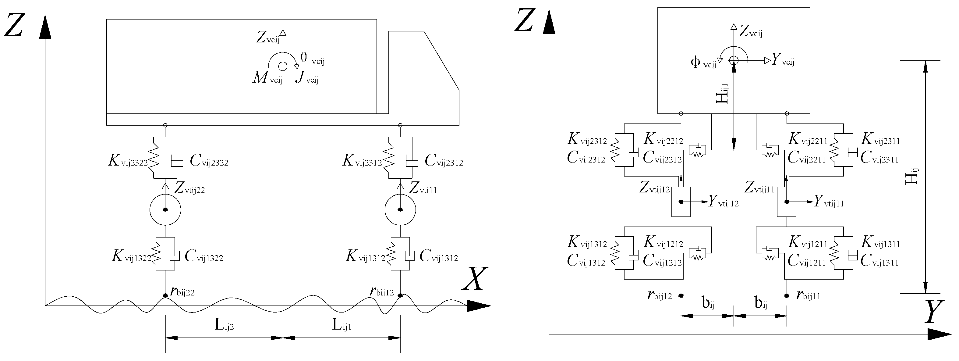
2.1. Automotive Dynamic Analysis Model

Vehicle models can be represented using rigid bodies, springs, dampers, and other elements. The main parameters include the number of rigid bodies, the number of springs, the mass of the rigid bodies, and the corresponding mass moments of inertia. By adjusting the combination of these parameters, various shapes of car models can be simulated.

Take a two-axis four-wheel car as an example [22]; it can be divided into five rigid bodies: the body and four wheels. These rigid bodies are connected through elastic and damping elements, as shown in Figure 1.

To simplify the calculation, considering that when the vehicle is traveling with a constant speed in a straight line, the vibration of each rigid body in the vehicle in the direction of the car’s travel has a negligible influence on both the bridge’s vertical and lateral vibration, the degrees of freedom (DOF) of each rigid body in the direction of the car’s motion can be ignored in the calculation. Therefore, the car body only considers five degrees of freedom; each wheel pair has two independent DOFs along the Y-axis displacement (Y) and the Z-axis displacement (Z). That is, four wheels have a total of eight DOFs. A two-axis four-wheel car has a total of 13 DOFs. Its displacement vector can be expressed as:

$$\begin{array}{c}{V}_{vij}\hfill \\ ={\left[Y_{vcij} Z_{vcij} {\varphi }_{vcij} {\theta }_{vcij} {\phi }_{vcij} Y_{vwij11} Z_{vwij11} Y_{vwij12} Z_{vwij12} Y_{vwij21} Z_{vwij21} Y_{vwij22} Z_{vwij22}\right]}^T\hfill \end{array}$$

(1)

where:$Y_{vcij}, Z_{vcij}, {\varphi }_{vcij}, {\theta }_{vcij} and {\phi }_{vcij}$ are the displacement of the y vehicle on the i lane along Y-axis, the displacement along Z-axis, the rotation angle around X-axis, the rotation angle around Y-axis, and the rotation angle around the Z-axis; and $Y_{vwij11}, Z_{vwij11}$ are the displacement of the right wheel and the left wheel of the front axle (the first axle) of the j vehicle on the i lane along Y-axis and Z-axis; and $Y_{vwij22}, Z_{vwij22}$ and $Y_{vwij21}, Z_{vwij21}$ are the displacement of the right wheel and the left wheel of the rear axle (the second axle) of j vehicle on the i lane along Y-axis and Z-axis. In

Table 1. Main parameters and descriptions of the vehicle dynamic analysis model.

Parameter	Description
$M_{vcij},\hspace{1em} J_{vczij}$	The rigid mass of the vehicle body of the j car on the i lane; The vertical rotational inertia of the vehicle body of the j car on the i lane.
$J_{vcxij},\hspace{1em} J_{vcyij}$	The lateral inertia of the vehicle body; The longitudinal rotational inertia of the vehicle body.
$K_{vj2211}, K_{vij2212}, K_{vij2221}, K_{vij2222}$	The lateral stiffness coefficient of secondary suspension.
$K_{vij2311}, K_{vij2312}, K_{vij2321}, K_{vij2322}$	The vertical stiffness coefficient of secondary suspension.
$C_{vj2211}, C_{vij2212}, C_{vij2221}, C_{vij2222}$	The lateral damping constant of each wheel.
$C_{vj2311}, C_{vij2312}, C_{vij2321}, C_{vij2322}$	The vertical damping constant of each wheel.
$M_{vwij11}, M_{vwij12}, M_{vwij21}, M_{vwij22}$	The vehicle’s unsprung mass.
$K_{vij1211}, K_{vij1212}, K_{vij1221}, K_{vij1222}$	The lateral stiffness coefficient of the vehicle’s wheel.
$K_{vij1311}, K_{vij1312}, K_{vij1321}, K_{vij1322}$	The vertical stiffness coefficient of the vehicle’s wheel.
$C_{vij1211}, C_{vij1212}, C_{vij1221}, C_{vij1222}$	The lateral damping constant of the vehicle’s wheel.
$C_{vij1311}, C_{vij1312}, C_{vij1321}, C_{vij1322}$	The vertical damping constant of the vehicle’s wheel.
$L_{ij1}, L_{ij2}$	The longitudinal distance from the vehicle’s first and second axles to the center of gravity of the car body.
$H_{ij1}, H_{ij}$	The distance from the vehicle body to the secondary suspension. The distance from the rigid body of the vehicle to the ground.

, the vehicle model’s parameters are shown.

Assuming that the car fits perfectly on the bridge’s top deck, the contact between the wheel and the top deck is point contact. In this case, the contact point displacement between the wheel and the bridge deck is affected by the displacement and the roughness.

Based on the above assumptions, take the vertical spring as an example to derive the relative displacement expression of the above two types of springs. Assuming there are $L_v$ lanes and $n_v$ vehicles on the $i$ lane, the relative displacement generated at the two ends of the vertical spring of the first type of spring (the spring connecting the vehicle body and the wheel) on the $j$ vehicle of the $i$ lane can be expressed as:

$$R_{vij23km}=Z_{vcij}+{\left(-1\right)}^{m+1}{b}_{ij}{\varphi }_{vcij}-{\left(-1\right)}^{k+1}{l}_{ijk}{\theta }_{vcij}-Z_{vwijkm}$$

(2)

where, $v$ is the vehicle; $c$ is the vehicle body; $w$ is the wheel; $i$ is the lane number; $j$ is the vehicle number; 2 is the second type spring (first type spring); 3 is the vertical spring; k is the axle number (k = 1, 2, 1 is the front axle and 2 is the rear axle); $m$ is the wheel number ($m$ = 1, 2, in the forward direction, 1 is the left wheel and 2 is the right wheel); $R_{vij23km}$ is the relative displacement of the second type vertical spring on the m wheel on k axle of j car on i lane; and $Z_{vwjkm}$ is the vertical displacement on the m wheel on k axle of j car on i lane.

The relative displacement at both ends of the spring connecting the wheels and the bridge top deck of the j car on the i lane can be expressed as:

$$R_{vij13km}=Z_{vwijkm}-V_{bzijkm}-r_{bzijkm}$$

(3)

where, $R_{vij13km}$ is the relative displacement of the primary vertical spring on k axle’s m wheel of j car on i lane; $Z_{vwjkm}$ is the vertical displacement on k axle’s m wheel of j car on i lane; $V_{bzijkm}$ is the vertical displacement of the bridge at the contact point of k axle’s m wheel of j car on i lane; and $r_{bzijkm}$ is the roughness value of the bridge deck at the contact point of k axle’s m wheel of j car on i lane.

$$\begin{array}{c}{V}_{bzijkm}={\left[N_1\left(x\right) dy{N}_5\left(x\right) N_2\left(x\right) N_3\left(x\right) dy{N}_6\left(x\right) N_4\left(x\right)\right]}_{x=x_c}\\ {\left[Z_{bijkm}^{ei} {\varphi }_{bijkm}^{ei} {\theta }_{bijkm}^{ei} Z_{bijkm}^{ej} {\varphi }_{bijkm}^{ej} {\theta }_{bijkm}^{ej}\right]}^T\end{array}$$

(4)

where, $Z_{bijkm}^{ei} {\varphi }_{bijkm}^{ei} {\theta }_{bijkm}^{ei}$ and $Z_{bijkm}^{ej} {\varphi }_{bijkm}^{ej} {\theta }_{bijkm}^{ej}$ are the vertical displacement, rotation around the X-axis, and rotation around the Y-axis at i and j end of the unit; x_c is the distance between the contact point and i end corresponding unit of the bridge; $dy$ is the y-coordinate difference between the contact point and the centroid of bridge unit in the global coordinate system; and $N_1\left(x\right),N_2\left(x\right),N_3\left(x\right),N_4\left(x\right),N_5\left(x\right),N_6\left(x\right)$ are girder element shape function, the expression can be found in references [1].

Similarly, the expression for the relative displacement between the two ends of a transverse spring can be obtained.

2.2. Vibration Equation of Vehicle Model

In the dynamic analysis model of the above car, taking the equilibrium state of the car under the action of its weight as the initial state, based on the virtual work conducted on the car’s inertial force, elastic force, and damping force, the vibration equation of the car can be obtained according to the principle of the following virtual work:

$$M_v{\ddot{v}}_v+C_v{\dot{v}}_v+K_v{v}_v=F_v$$

(5)

where, $M_v, C_v, and K_v$ are the mass, damping, and stiffness matrix for the vehicle, respectively; $v_v$, ${\dot{v}}_v$, and ${\ddot{v}}_v$ are the absolute displacement, velocity, and acceleration arrays of the vehicle, respectively; and $F_v$ is the array of external loads on the vehicle and is mainly the force between the bridge and the wheel contact point, without considering the vehicle’s weight.

Here, the vibration equation of the vehicle described above is established in its coordinate system. However, when the vehicle runs on a curved bridge, the coordinate system changes depending on the vehicle’s location. Therefore, in each time step, the motion equation of the car needs to be converted to the global coordinate system.

• Formation of stiffness matrix

The stiffness matrix of a vehicle is related to the virtual work via the elastic forces, which depends on the relative deformation of the two ends of the spring. Each two-axle vehicle has four lateral and four vertical springs between the vehicle body and the wheels. Taking the lateral spring as an example, we can obtain.

$$R_{vij2211}=Y_{vcij}+H_{ij1}{\phi }_{vcij}+l_{ij1}{\varphi }_{vcij}-Y_{vwij11}$$

(6)

$$R_{vij2212}=Y_{vcij}+H_{ij1}{\phi }_{vcij}+l_{ij1}{\varphi }_{vcij}-Y_{vwij11}$$

(7)

$$R_{vij2221}=Y_{vcij}+H_{ij2}{\phi }_{vcij}+l_{ij2}{\varphi }_{vcij}-Y_{vwij21}$$

(8)

$$R_{vij2222}=Y_{vcij}+H_{ij2}{\phi }_{vcij}+l_{ij2}{\varphi }_{vcij}-Y_{vwij22}$$

(9)

The virtual work made via the elastic force of the horizontal spring is:

$$\begin{array}{cc}\hfill \delta W_{S2}^V={\displaystyle {\displaystyle \sum }_{k=1}^2}{\displaystyle {\displaystyle \sum }_{m=1}^2}& \left(K_{vij22km}{R}_{vij22km}\delta R_{vij22km}\right)={\displaystyle {\displaystyle \sum }_{k=1}^2}{\displaystyle {\displaystyle \sum }_{m=1}^2}\{K_{vij22km}[Y_{vcij}+H_{ij1}{\phi }_{vcij}\hfill \\ & +{\left(-1\right)}^{k+1}{l}_{ijk}{\varphi }_{vcij}-Y_{vwijkm}\left]\right[\delta Y_{vcij}+H_{ij1}\delta {\phi }_{vcij}\hfill \\ & +{\left(-1\right)}^{k+1}{l}_{ijk}\delta {\varphi }_{vcij}-\delta Y_{vwijkm}\left]\right\}\hfill \end{array}$$

(10)

Taking the lateral spring of the left wheel (m = 1) of the front axle (k = 1) as an example, substituting Equation (6) into Equation (10), there is:

$$\begin{array}{c}{K}_{vij2211}{R}_{vij2211}\delta R_{vij2211}=K_{vij2211}\left(Y_{vcij}+H_{ij1}{\phi }_{vcij}+l_{ij1}{\varphi }_{vcij}-Y_{vwij11}\right)\delta \left(Y_{vcij}+H_{ij1}{\phi }_{vcij}+l_{ij1}{\varphi }_{vcij}-Y_{vwij11}\right)\\ =(K_{vij2211}{Y}_{vcij}\delta Y_{vcij}+K_{vij2211}{H}_{ij1}{Y}_{vcij}\delta Y_{vcij}+K_{vij2211}{l}_{ij1}{Y}_{vcij}\delta Y_{vcij}-K_{vij2211}{Y}_{vcij}\delta Y_{vwij11}+\\ K_{vij2211}{H}_{ij1}{\phi }_{vcij}{Y}_{vcij}+K_{vij2211}{H_{ij1}}^2{\phi }_{vcij}\delta Y_{vcij}+K_{vij2211}{H}_{ij1}{l}_{ij1}{\phi }_{vcij}\delta {\varphi }_{vcij}-K_{vij2211}{H}_{ij1}{\phi }_{vcij}\delta Y_{vwij11}+\\ K_{vij2211}{l}_{ij1}{\varphi }_{vcij}\delta Y_{vcij}+K_{vij2211}{l}_{ij1}{H}_{ij1}{\varphi }_{vcij}\delta {\phi }_{vcij}+K_{vij2211}{l_{ij1}}^2{\varphi }_{vcij}\delta {\varphi }_{vcij}-K_{vij2211}{l}_{ij1}{\varphi }_{vcij}\delta Y_{vwij11}-\\ K_{vij2211}{Y}_{vwij11}\delta Y_{vcij}-K_{vij2211}{H}_{ij1}{Y}_{vwij11}\delta {\phi }_{vcij}-K_{vij2211}{l}_{ij1}{Y}_{vwij11}\delta {\varphi }_{vcij}+K_{vij2211}{Y}_{vwij11}\delta Y_{vwij11}\end{array}$$

(11)

where the polynomial on the right side consists of monomials similar to kuδu, k is the constant coefficient of the monomial, and u is the displacement corresponding to the independent degree of freedom of the vehicle. According to the “right seating” rule [19], the coefficient k is placed in the matrix corresponding to the “row” of DOF related to δu and the “column” of DOF related to u, resulting in the following submatrix form:

$$\begin{array}{ccccc}& \begin{array}{c}{Y}_{vcij}\hfill \end{array}& \begin{array}{c}{\phi }_{vcij}\hfill \end{array}& \begin{array}{c}{\varphi }_{vcij}\hfill \end{array}& \begin{array}{c}{Y}_{vwij11}\hfill \end{array}\\ \begin{array}{c}\delta Y_{vcij}\\ \delta {\phi }_{vcij}\\ \delta {\varphi }_{vcij}\\ \delta Y_{vwij11}\end{array}& [\begin{array}{c}{K}_{vij2211}\\ K_{vij2211}{H}_{ij1}\\ K_{vij2211}{l}_{ij1}\\ -K_{vij2211}\end{array}& \begin{array}{c}{K}_{vij2211}{H}_{ij1}\\ K_{vij2211}{H_{ij1}}^2\\ K_{vij2211}{l}_{ij1}{H}_{ij1}\\ -K_{vij2211}{H}_{ij1}\end{array}& \begin{array}{c}{K}_{vij2211}{l}_{ij1}\\ K_{vij2211}{l}_{ij1}{H}_{ij1}\\ K_{vij2211}{l_{ij1}}^2\\ -K_{vij2211}{l}_{ij1}\end{array}& \begin{array}{c}-K_{vij2211}\\ -K_{vij2211}{H}_{ij1}\\ -K_{vij2211}{l}_{ij1}\\ K_{vij2211}\end{array}]\end{array}$$

(12)

Similarly, by substituting Equations (7)–(9) into Equation (10), respectively, a submatrix form similar to Equation (12) is achieved. The stiffness matrix of a single two-axle vehicle is obtained by superimposing and combining all submatrices. By collecting the stiffness matrices of all vehicles, the stiffness matrix of the vehicle fleet is obtained.

• Formation of damping matrix

The damping matrix of a vehicle is related to the virtual work made by the damping force, which is determined via the relative velocity between the two ends of the damping element. Each two-axle vehicle has four lateral and vertical damping elements between the vehicle body and the wheels. Taking the vertical damping element as an example, we can obtain:

$${\dot{R}}_{vij2311}={\dot{Z}}_{vcij}+b_{ij}{\dot{\phi }}_{vcij}-l_{ij1}{\dot{\theta }}_{vcij}-{\dot{Z}}_{vwij11}$$

(13)

$${\dot{R}}_{vij2311}={\dot{Z}}_{vcij}-b_{ij}{\dot{\phi }}_{vcij}-l_{ij1}{\dot{\theta }}_{vcij}-{\dot{Z}}_{vwij11}$$

(14)

$${\dot{R}}_{vij2311}={\dot{Z}}_{vcij}+b_{ij}{\dot{\phi }}_{vcij}+l_{ij1}{\dot{\theta }}_{vcij}-{\dot{Z}}_{vwij11}$$

(15)

$${\dot{R}}_{vij2311}={\dot{Z}}_{vcij}-b_{ij}{\dot{\phi }}_{vcij}+l_{ij1}{\dot{\theta }}_{vcij}-{\dot{Z}}_{vwij11}$$

(16)

The virtual work achieved via the damping force of the vertical damping element was:

$$\begin{array}{cc}\hfill \delta W_{S3}^V={\displaystyle {\displaystyle \sum }_{k=1}^2}{\displaystyle {\displaystyle \sum }_{m=1}^2}& \left(C_{vij23km}{\dot{R}}_{vij23km}\delta R_{vij23km}\right)={\displaystyle {\displaystyle \sum }_{k=1}^2}{\displaystyle {\displaystyle \sum }_{m=1}^2}\{C_{vij23km}\left[{\dot{Z}}_{vcij}+{\left(-1\right)}^{k+1}{l}_{ijk}{\dot{\theta }}_{vcij}-{\dot{Z}}_{vwijkm}\right][\delta Y_{vcij}\hfill \\ & +H_{ij1}\delta {\phi }_{vcij}+{\left(-1\right)}^{k+1}{l}_{ijk}\delta {\varphi }_{vcij}-\delta Y_{vwijkm}\left]\right\}\hfill \end{array}$$

(17)

Taking the vertical spring of the left wheel (m = 1) of the front axle (k = 1) as an example, substituting Equation (6) into Equation (10), there is:

$$\begin{array}{c}{C}_{vij2311}{\dot{R}}_{vij2311}\delta {\dot{R}}_{vij2311}=C_{vij2311}\left({\dot{Z}}_{vcij}+b_{ij}{\dot{\phi }}_{vcij}-l_{ij1}{\dot{\theta }}_{vcij}-{\dot{Z}}_{vwij11}\right)\delta \left(Z_{vcij}+b_{ij}{\phi }_{vcij}-l_{ij1}{\theta }_{vcij}-Z_{vwij11}\right)\\ =(C_{vij2311}{\dot{Z}}_{vcij}\delta Z_{vcij}+C_{vij2311}{b}_{ij}{\dot{Z}}_{vcij}\delta {\phi }_{vcij}-c_{vij2311}{l}_{ij1}{\dot{Z}}_{vcij}\delta {\theta }_{vcij}-C_{vij2311}{\dot{Z}}_{vcij}\delta Z_{vwij11}+\\ C_{vij2311}{b}_{ij}{\dot{\phi }}_{vcij}\delta Z_{vcij}+C_{vij2311}{b_{ij}}^2{\dot{\phi }}_{vcij}\delta {\phi }_{vcij}-C_{vij2311}{b}_{ij}{l}_{ij}{\dot{\phi }}_{vcij}\delta {\theta }_{vcij}-C_{vij2311}{b}_{ij}{\dot{\phi }}_{vcij}\delta Z_{vwij11}-\\ C_{vij2311}{l}_{ij1}{\dot{\theta }}_{vcij}\delta Z_{vcij}-C_{vij2311}{l}_{ij1}{b}_{ij1}{\dot{\theta }}_{vcij}\delta {\phi }_{vcij}+C_{vij2311}{l_{ij1}}^2{\dot{\theta }}_{vcij}\delta {\theta }_{vcij}+C_{vij2311}{l}_{ij1}{\dot{\theta }}_{vcij}\delta Z_{vwij11}-\\ C_{vij2311}{\dot{Z}}_{vwij11}\delta Z_{vcij}-C_{vij2311}{b}_{ij}{\dot{Z}}_{vwij11}\delta {\phi }_{vcij}+C_{vij2311}{l}_{ij1}{\dot{Z}}_{vwij11}\delta {\theta }_{vcij}+C_{vij2311}{\dot{Z}}_{vwij11}\delta Z_{vwij11}\end{array}$$

(18)

where, the polynomial on the right side consists of monomials similar to c$\dot{u}$δu, $c$ is the constant coefficient of the monomial, $\dot{u}$ is the speed corresponding to the independent DOF of the vehicle, and $u$ is the displacement corresponding to the independent degree of freedom of the vehicle. According to the “right seating” rule [19], the coefficient $c$ is placed in the matrix corresponding to the “row” of DOF related to $\delta u$ and the “column” of DOF related to $\dot{u}$, resulting in the following submatrix form:

$$\begin{array}{ccccc}& \begin{array}{c}{\dot{Z}}_{vcij}\hfill \end{array}& \begin{array}{c}{\dot{\phi }}_{vcij}\hfill \end{array}& \begin{array}{c}{\dot{\theta }}_{vcij}\hfill \end{array}& \begin{array}{c}{\dot{Z}}_{vwij11}\hfill \end{array}\\ \begin{array}{c}\delta Z_{vcij}\\ \delta {\phi }_{vcij}\\ \delta {\varphi }_{vcij}\\ \delta Z_{vwij11}\end{array}& [\begin{array}{c}{C}_{vij2311}\\ C_{vij2311}{b}_{ij}\\ -C_{vij2311}{l}_{ij1}\\ -C_{vij2311}\end{array}& \begin{array}{c}{C}_{vij22311}{b}_{ij}\\ C_{vij2311}{b_{ij}}^2\\ -C_{vij2311}{b}_{ij1}{l}_{ij}\\ -C_{vij2311}{b}_{ij}\end{array}& \begin{array}{c}-C_{vij2311}{l}_{ij1}\\ -C_{vij2311}{l}_{ij}{b}_{ij1}\\ C_{vij2311}{l_{ij1}}^2\\ C_{vij2311}{l}_{ij1}\end{array}& \begin{array}{c}-C_{vij2311}\\ -C_{vij2311}{b}_{ij}\\ C_{vij2311}{l}_{ij1}\\ C_{vij2311}\end{array}]\end{array}$$

(19)

Similarly, by substituting Equations (14)–(16) into Equation (17), respectively, a submatrix form similar to Equation (19) is achieved. The damping matrix of a single two-axle vehicle is obtained via superimposing and combining all submatrices. By collecting the stiffness matrices of all vehicles, the damping matrix $C_v$ of the vehicle fleet is obtained.

• Formation of quality matrix

The mass matrix of a vehicle is related to the virtual work achieved via inertial forces, which is determined by the acceleration at each mass point. Each two-axle vehicle has a body and four wheels for five rigid body mass points. The mass matrix of a single two-axle vehicle is obtained, as shown in Equation (20).

$$M_v=\left[\begin{array}{ccccccccccccc}{M}_{vcij}& & & & & & & & & & & & \\ & M_{vcij}& & & & & & & & & & & \\ & & J_{vcxij}& & & & & & & & & & \\ & & & J_{vcyij}& & & & & & & & & \\ & & & & J_{vczij}& & & & & & & & \\ & & & & & M_{vwij11}& & & & & & & \\ & & & & & & M_{vwij11}& & & & & & \\ & & & & & & & M_{vwij12}& & & & & \\ & & & & & & & & M_{vwij12}& & & & \\ & & & & & & & & & M_{vwij21}& & & \\ & & & & & & & & & & M_{vwij21}& & \\ & & & & & & & & & & & M_{vwij22}& \\ & & & & & & & & & & & & M_{vwij22}\end{array}\right]$$

(20)

Combining all of the car quality matrices, the vehicle quality matrix $M_v$ can be obtained.

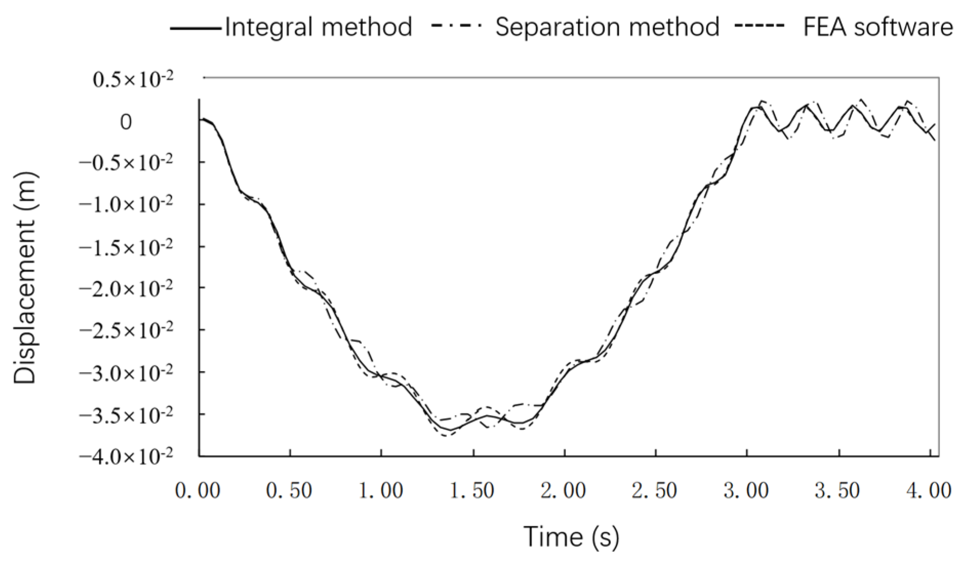
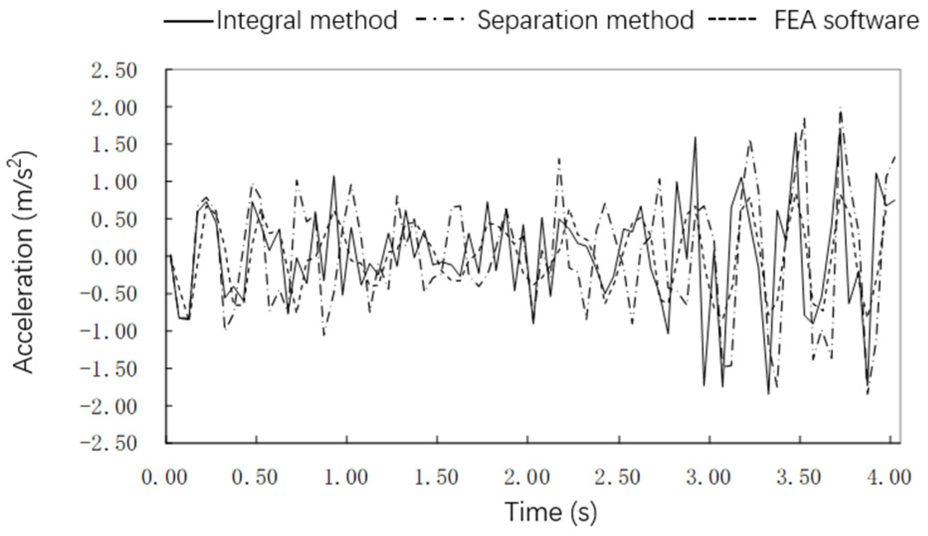
3. Verification of Programs

This module is mainly used to analyze vehicle-bridge coupling vibration, which can be utilized to analyze vehicle-bridge coupling vibration when a single type of vehicle passes through a bridge. It can also calculate the vehicle-bridge coupling vibration response of multiple routes and fleets with different speeds under different bridge surface irregularities. It can also perform vehicle-bridge coupling vibration analysis for one-way and two-way driving.

A simple-supported curved box girder bridge was taken as the research object; the main parameters were as follows: calculated span L = 24.0 m, girder radius R = 100.0 m, elastic modulus E = 3.250 × 1010 N/m², shear modulus G = 1.350 × 1010 N/m², and density ρ = 2600 kg/m³. The main girder’s cross-section was a single box single chamber with a cross-sectional area of A = 4.392 m², a cross-sectional moment of inertia I_y = 2.443 m⁴, I_z = 20.721 m⁴, and a free torsional moment of inertia J = 5.042 m⁴. The main girder section is shown in Figure 2.

Assuming the spring-mass system as shown in Figure 3, the suspended mass of the moving mass block was $M=102,041 \mathrm{kg}$, the spring stiffness supporting the mass block was $K=1.0\times {10}^{10} \mathrm{kN}·\mathrm{m}$, and the spring-mass block travelled through the simple-supported girder bridge with a constant speed, the system speed was the $V=36 \mathrm{km}/\mathrm{h}$. The displacement and acceleration time histories at the simple-supported bridge mid-span were calculated using this program’s integral method, separation method, and finite element analysis software, as shown in Figure 4 and Figure 5.

Comparing the results in Figure 4 and Figure 5, the overall and separate methods in the program Cmck in this article agreed well with the results calculated via the common FEA (Ansys 17.0) software, indicating that the calculation program based on the two methods of overall and separate v coupled vibration analysis can be used for vibration analysis of time-varying vehicle-bridge coupled systems.

4. Spatial Vibration Analysis of the Coupled Time-Varying System of Vehicle-Curved Girder Bridge

A three-span curved continuous box-girder bridge with an equal cross-section was taken as the research object; different types of unit were used to build the finite element calculation model of the highway curved girder bridge. The model was built in the Cmck program, which is a vibration analysis program for highway bridge vehicle bridge coupling time-varying systems, and has multiple functions, including static analysis of structures, natural vibration characteristics analysis, dynamic analysis of moving loads, and vehicle bridge coupling vibration analysis. Based on the vehicle-bridge mentioned above, the coupling vibration analysis method, and the compiled computational program Cmck, the vehicle-bridge coupling spatial vibration simulation analysis of the highway curved girder bridge was performed and the dynamic responses of the coupled time-varying system with different conditions were calculated. The influence of the main parameters such as curvature radius, different curved beam unit types, constraint conditions, and vehicle types on the coupling spatial vibration of the curved girder bridge were discussed.

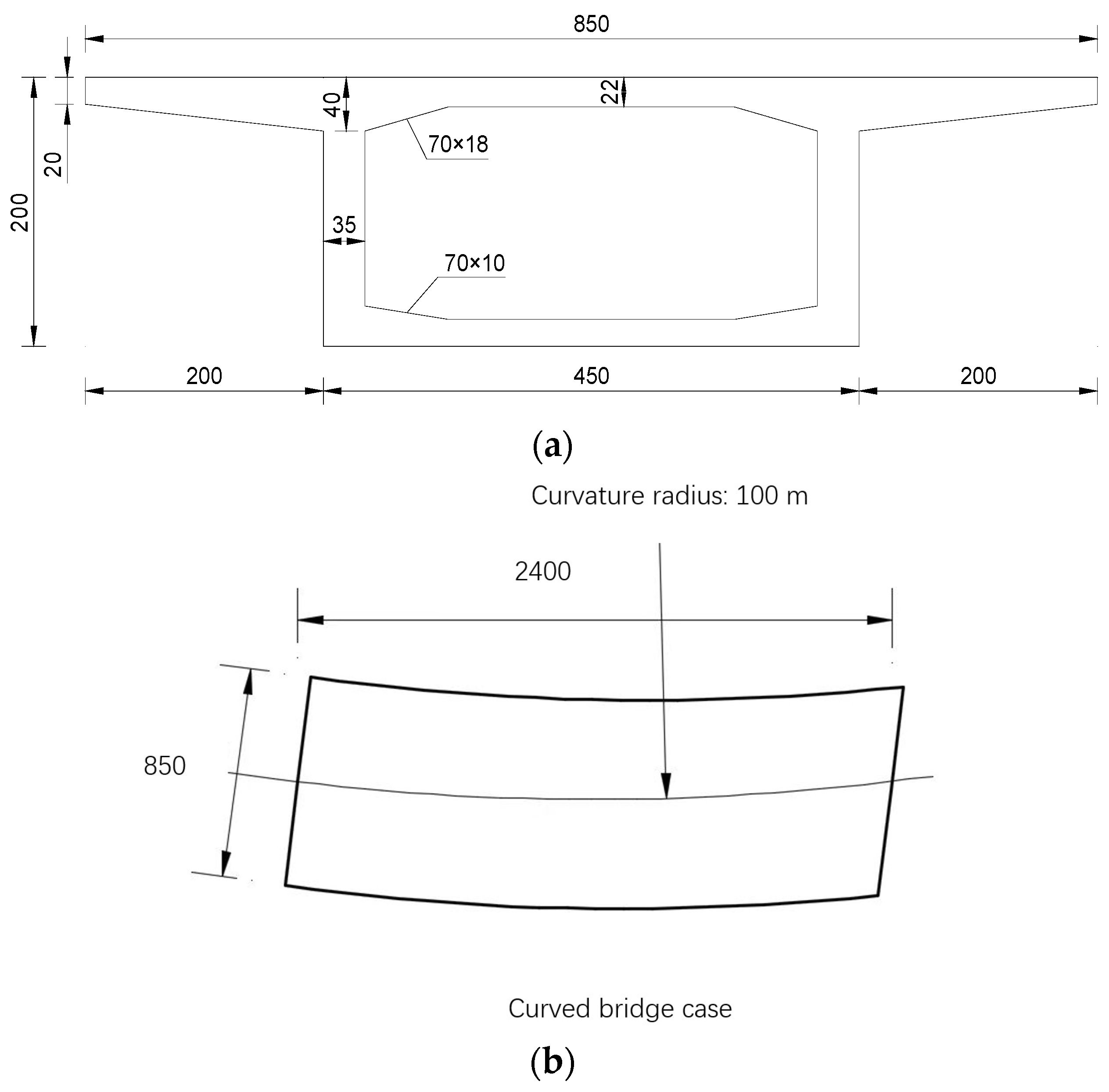
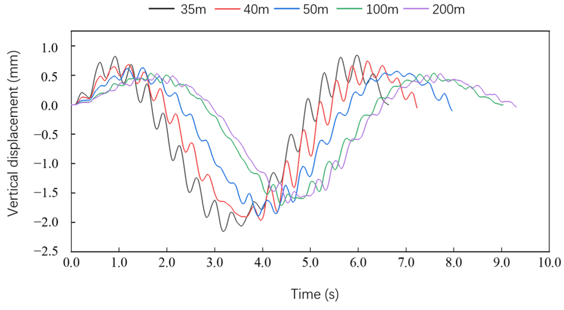
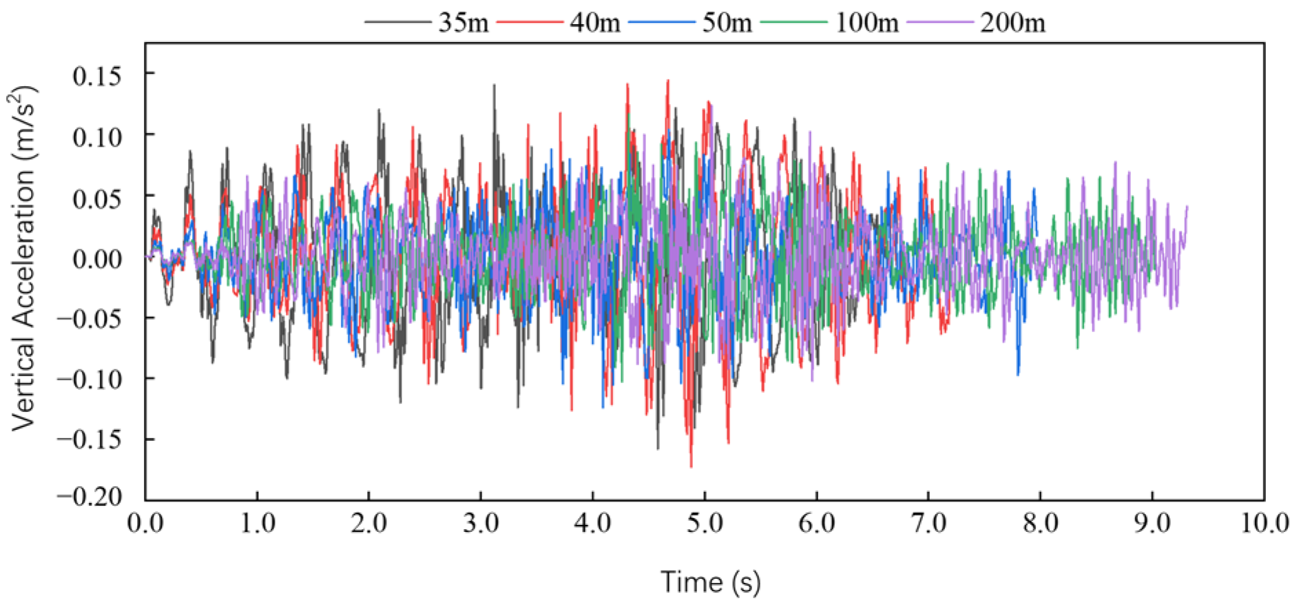
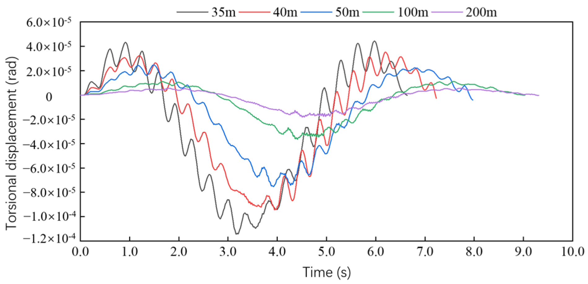
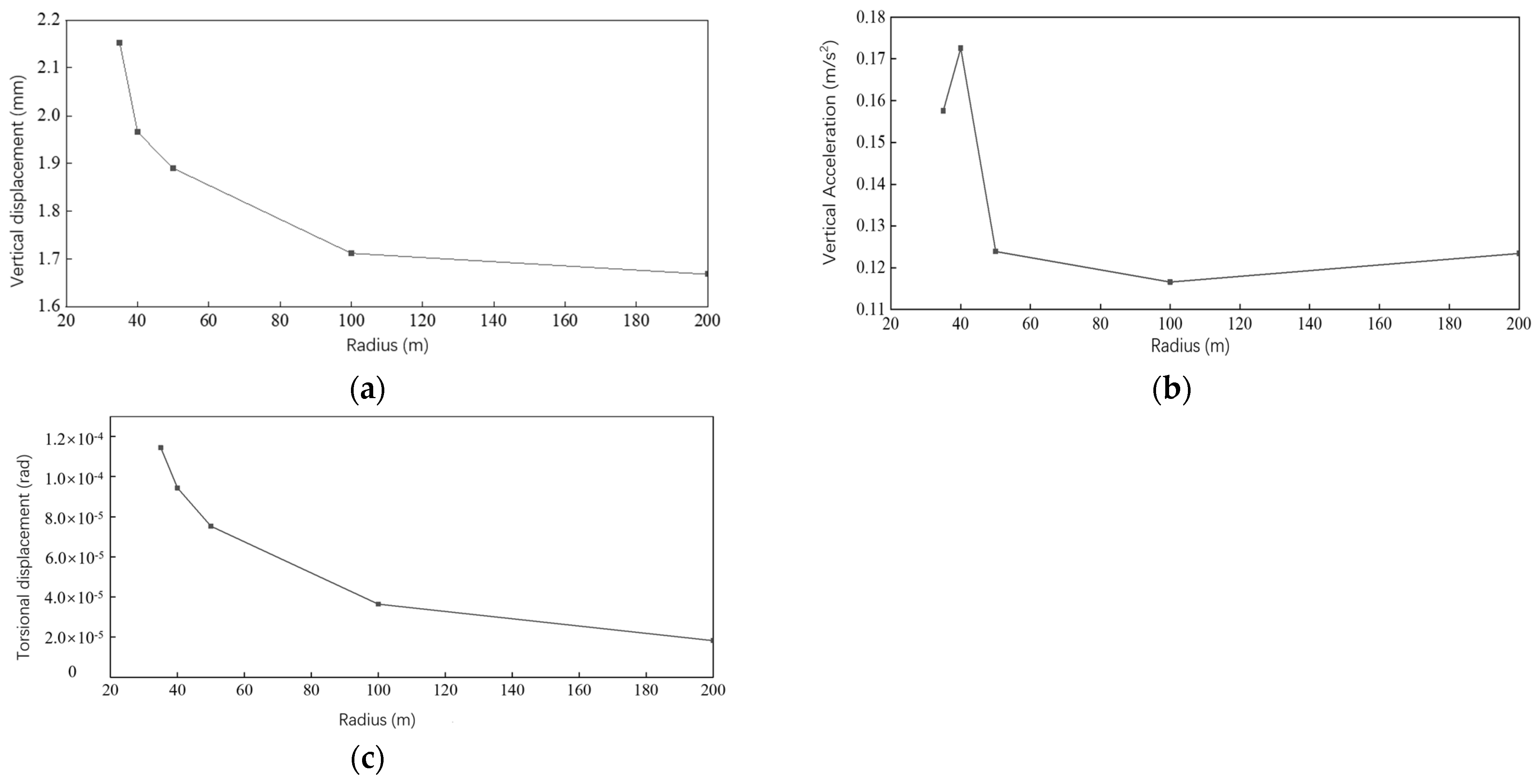
4.1. Impact Analysis of Curvature Radius

Based on the above bridge and car models, according to the common radius values of highway and urban interchange ramp bridges, the curvature radii were selected as 35m, 40 m, 500 m, 100 m, and 200 m, respectively. With the same bridge length, the Timoshenko curved beam element was used to discretize the bridge structure. Considering the good bridge top deck irregularity level, the self-written program Cmck was used to calculate the coupling dynamic responses when a stranded truck with a load of 1 ton travelled through the curved girder bridge at a speed of 40 km/h and explored the influence of curvature radius on the spatial vibration.

The comparison of the displacement and the acceleration time-history responses at the bridge mid-span with different radii of curvature are shown in Figure 6, Figure 7 and Figure 8. The peak values at the mid-span are shown in

Table 2. Comparison of dynamic response peak values of bridges with different curvature radii.

Radius  (m)	Vertical Displacement (mm)	Vertical Acceleration (m/s2)	Torsional Displacement (rad)
35	2.153	0.158	0.114 × 10−3
40	1.966	0.173	0.944 × 10−4
50	1.890	0.124	0.753 × 10−4
100	1.712	0.117	0.364 × 10−4
200	1.668	0.123	0.183 × 10−4

and Figure 9.

From Figure 6, Figure 7, Figure 8 and Figure 9 and Table 2, as the radius of curvature increased, the dynamic responses showed a gradual decrease. The peak vertical displacement decreased from 2.153 mm to 1.668 mm, a decrease of 22.3%; the peak vertical acceleration decreased from 0.173 m/s² to 0.123 m/s², a decrease of 28.9%; the peak torsional angular displacement decreased from 0.114 × 10⁻³ rad to 0.183 × 10⁻⁴ rad, a decrease of 83.9%. Within the radius of curvature less than 100m, the decrease in the dynamic responses was more pronounced. Compared with the vertical dynamic response, the torsional response was more sensitive to the radius of curvature.

4.2. Analysis of the Influence of Constraint Methods

Two types of constraints were selected. One was to set the boundary conditions of the bridge model to the general constraint arrangement of straight bridges in a rectangular coordinate system, similar to the general support constraints of a common straight bridge, i.e., constraining the nodes’ degrees of freedom in the overall coordinate system (short as the rectangular coordinate system in the following text). The other was to set the boundary conditions of the curved girder bridge by setting rigid connections in the radial and standard directions of the fulcrum in a polar coordinate system (short as the polar coordinate system in the following text). Based on the above bridge and vehicle models, the Timoshenko curved beam element was utilized to discretize the structure, and the self-written program was used to consider the good-grade deck roughness. The vehicle-bridge coupled dynamic response was calculated when a heavy truck with a speed of 40 km/h passed through the curved bridge, and the influence of constraint ways on the vehicle-bridge coupled vibration of the bridge was discussed.

The comparison of the indexes such as the displacement and the acceleration time-history responses in the mid-span of bridges under different restraint modes is in Figure 10, Figure 11 and Figure 12, and the comparison of peak responses in the mid-span of bridges is summarized in

Table 3. Comparison of dynamic response peaks of bridges under different constraints.

Constraints Arrangement	Vertical Displacement (mm)	Vertical Acceleration (m/s2)	Torsional Displacement (rad)
Polar coordinate	1.890	0.124	0.753 × 10−4
Rectangular coordinate	5.756	0.363	0.113 × 10−3

.

As shown in Figure 10, Figure 11 and Figure 12 and Table 2, different constraint methods of the bridge significantly affect bridge dynamic responses. Compared to the polar coordinate system, the bridge vertical and torsional dynamic responses under the rectangular coordinate system constraint were more extensive, with the vertical displacement peak increasing from 1.890 mm to 5.756 mm, the vertical acceleration peak increasing from 0.124 m/s² to 0.363 m/s², and the torsional displacement peak increasing from 0.753 ×10⁻⁴ rad to 0.113 ×10⁻³ rad.

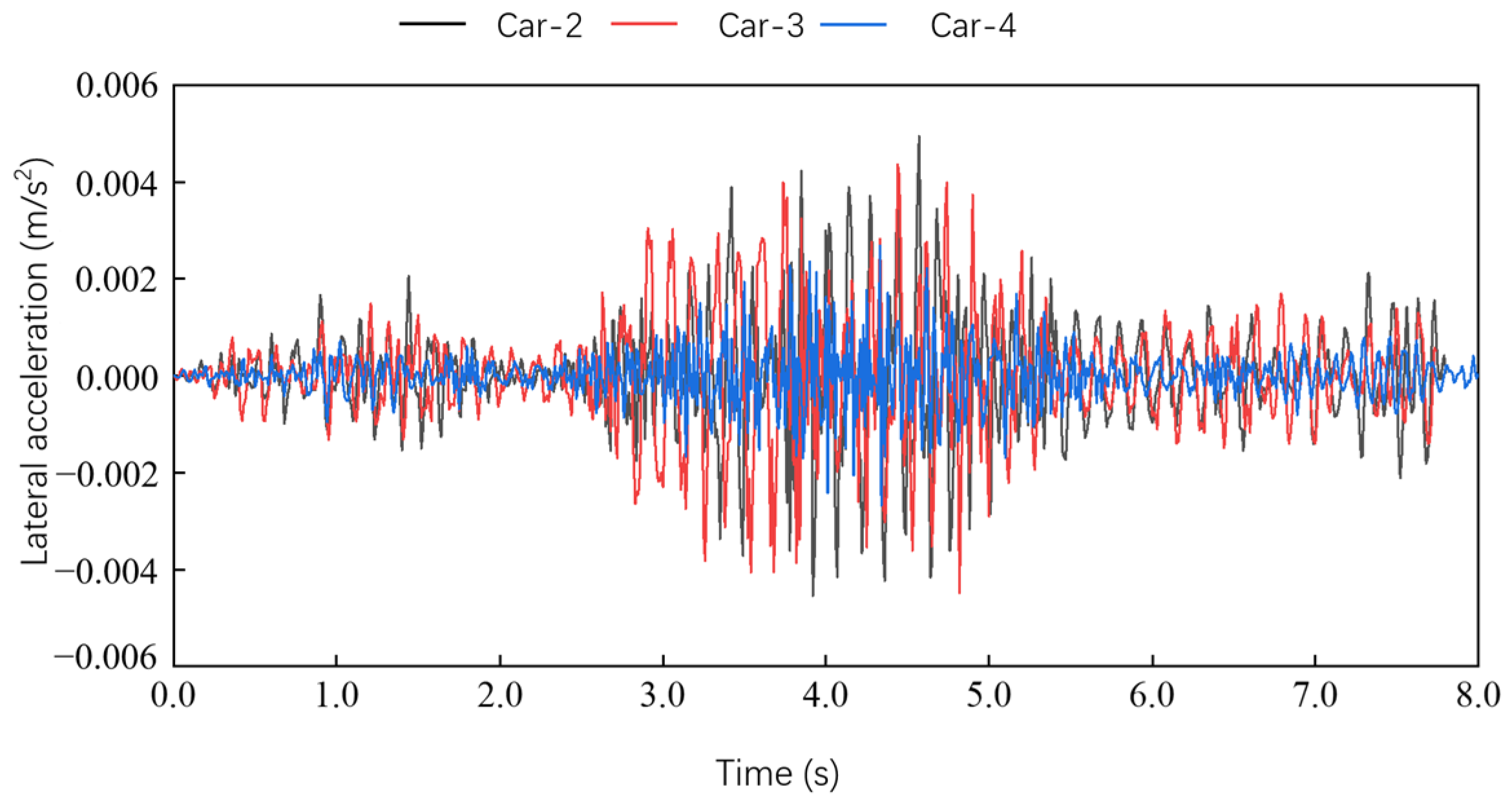
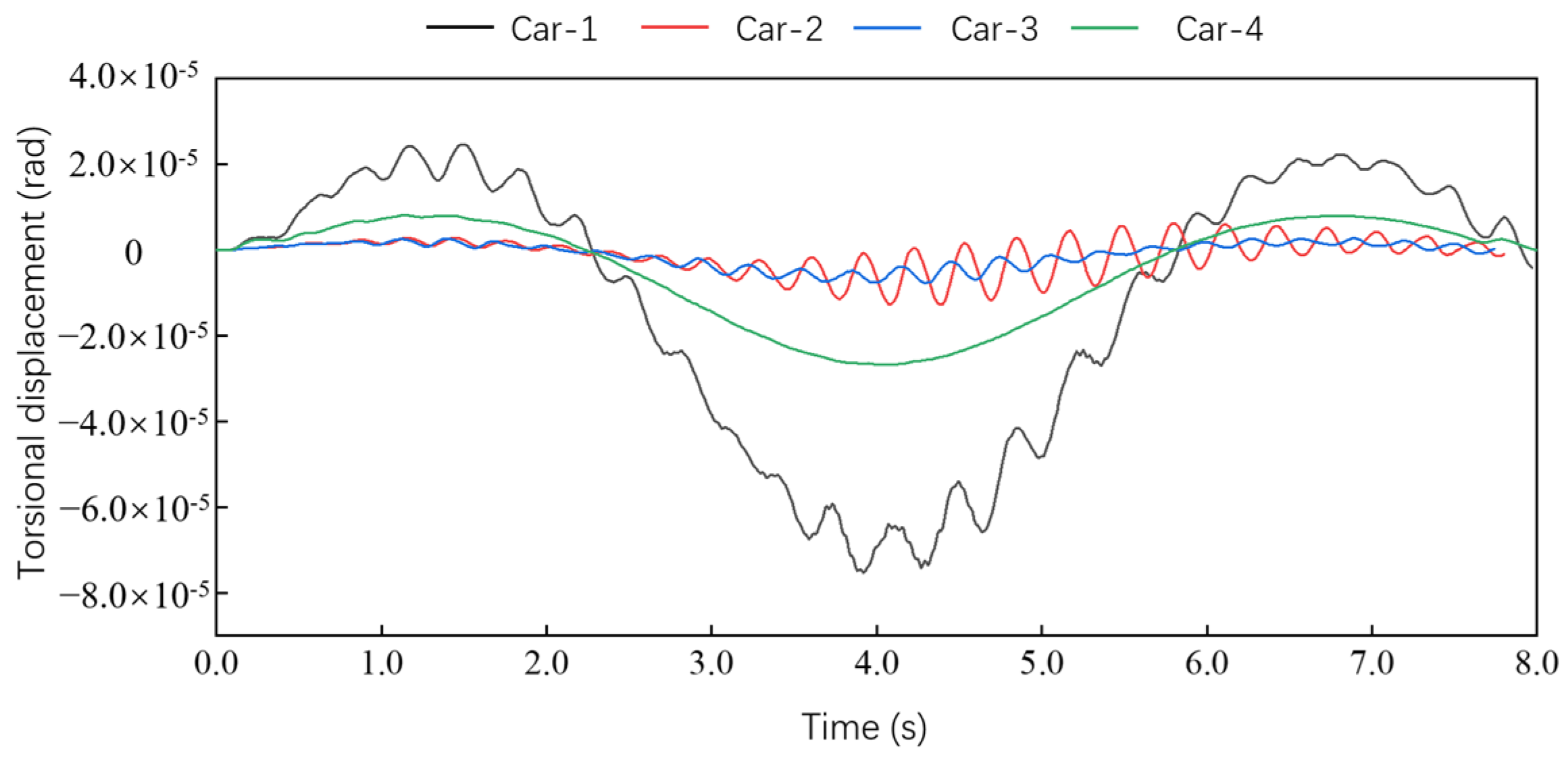
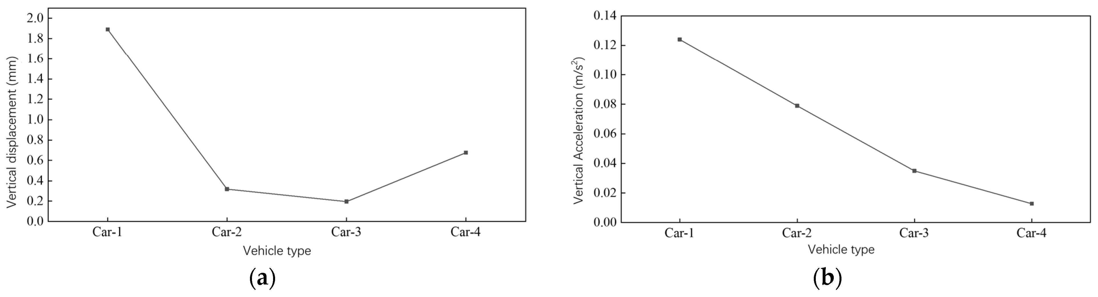
4.3. Analysis of the Impact of Vehicle Types

Four common vehicle models were selected: heavy trucks, Santana cars, FAW Jiabao, and box trucks, named Car-1, Car-2, Car-3, and Car-4 [23], respectively. Considering the good level of deck irregularity, the Timoshenko curved beam element was used to discretize the structure. A self-written calculation program was made to get the vehicle-bridge coupled dynamic response of a car traveling at a constant speed of 40 km/h through a curved girder bridge and to analyze the impact of vehicle type on the vehicle-bridge coupled vibration of curved bridges.

The comparison diagrams of both displacement and acceleration response time-history curves at the mid-span of bridges under different vehicle types are shown in Figure 13, Figure 14, Figure 15, Figure 16 and Figure 17, and the comparisons of peak responses at the mid-span of bridges are shown in

Table 4. The dynamic response peak of bridges under different vehicle types.

Vehicle Type	Vertical Displacement (mm)	Vertical Acceleration (m/s2)	Lateral Displacement (mm)	Lateral Acceleration (m/s2)	Torsional Displacement (rad)
Car-1	1.890	0.124	--	--	0.753 × 10−4
Car-2	0.318	0.079	3.449	0.747	0.128 × 10−4
Car-3	0.196	0.035	5.898	1.017	0.774 × 10−5
Car-4	0.675	0.013	1.913`	0.034	0.269 × 10−4

and Figure 18.

From Table 4 and Figure 13, Figure 14, Figure 15, Figure 16, Figure 17 and Figure 18, under the action of different vehicle types, the order of axial weight was Car-1, Car-4, Car-2, and Car-3. As the vehicle axle weight decreased, the vertical and torsional dynamic responses in the bridge span decreased while the lateral dynamic response gradually increased. The vertical displacement decreased from 1.89 mm to 0.20 mm; the vertical acceleration decreased from 0.12 m/s² to 0.03 m/s², the lateral displacement increased from 1.91 mm to 5.90 mm, and the lateral acceleration increased from 0.03 m/s² to 1.02 m/s².

5. Conclusions

This article took a three-span curved uniform section continuous box girder bridge as the research object. It used Fortran language to develop a highway bridge vehicle-bridge coupling vibration analysis program called Cmck. The influence laws of curvature radius, constraint method, and vehicle type on the vehicle-bridge coupling vibration of highway curved girder bridges were explored. The results showed that:

(1)

Through comparison with the results of general finite element program calculations, it was shown that the overall and separate methods in the program Cmck had good agreement with the results via general FEA software, indicating that the calculation program based on the two methods of overall and separate vehicle-bridge coupled vibration analysis can effectively analyze the vibration.

(2)

As the radius of curvature increased, the dynamic response of the bridge showed a gradual decreasing trend. The peak vertical displacement decreased by 22.3%, the peak vertical acceleration decreased by 28.9%, and the peak torsional angular displacement decreased by 83.9%. Within the radius of curvature less than 100m, the decrease in the dynamic response of the bridge was more pronounced; compared to the vertical dynamic response, the torsional response was more sensitive to the radius of curvature.

(3)

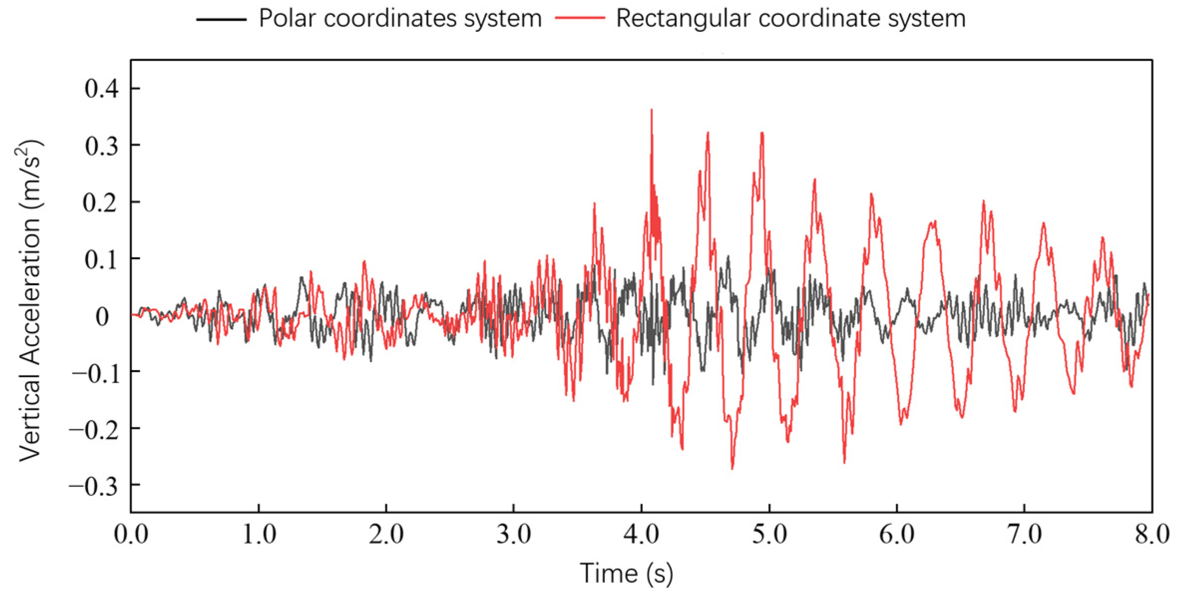
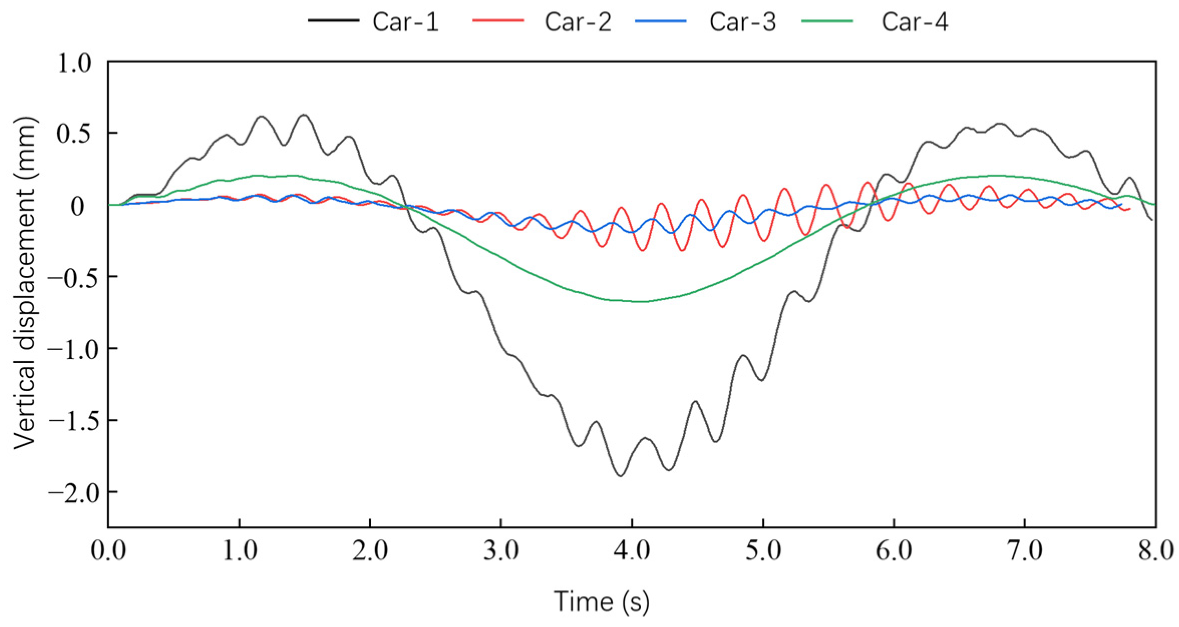
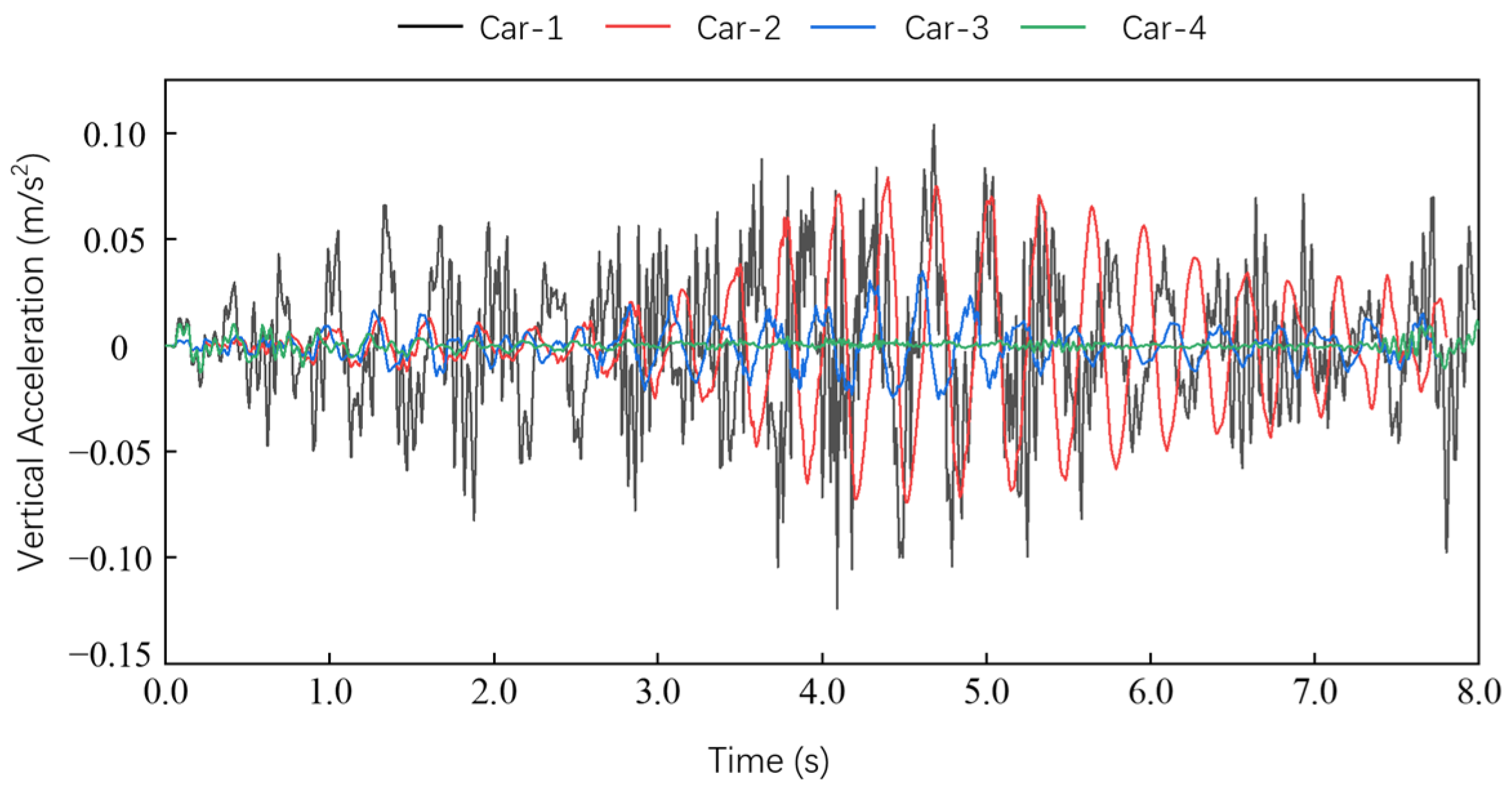
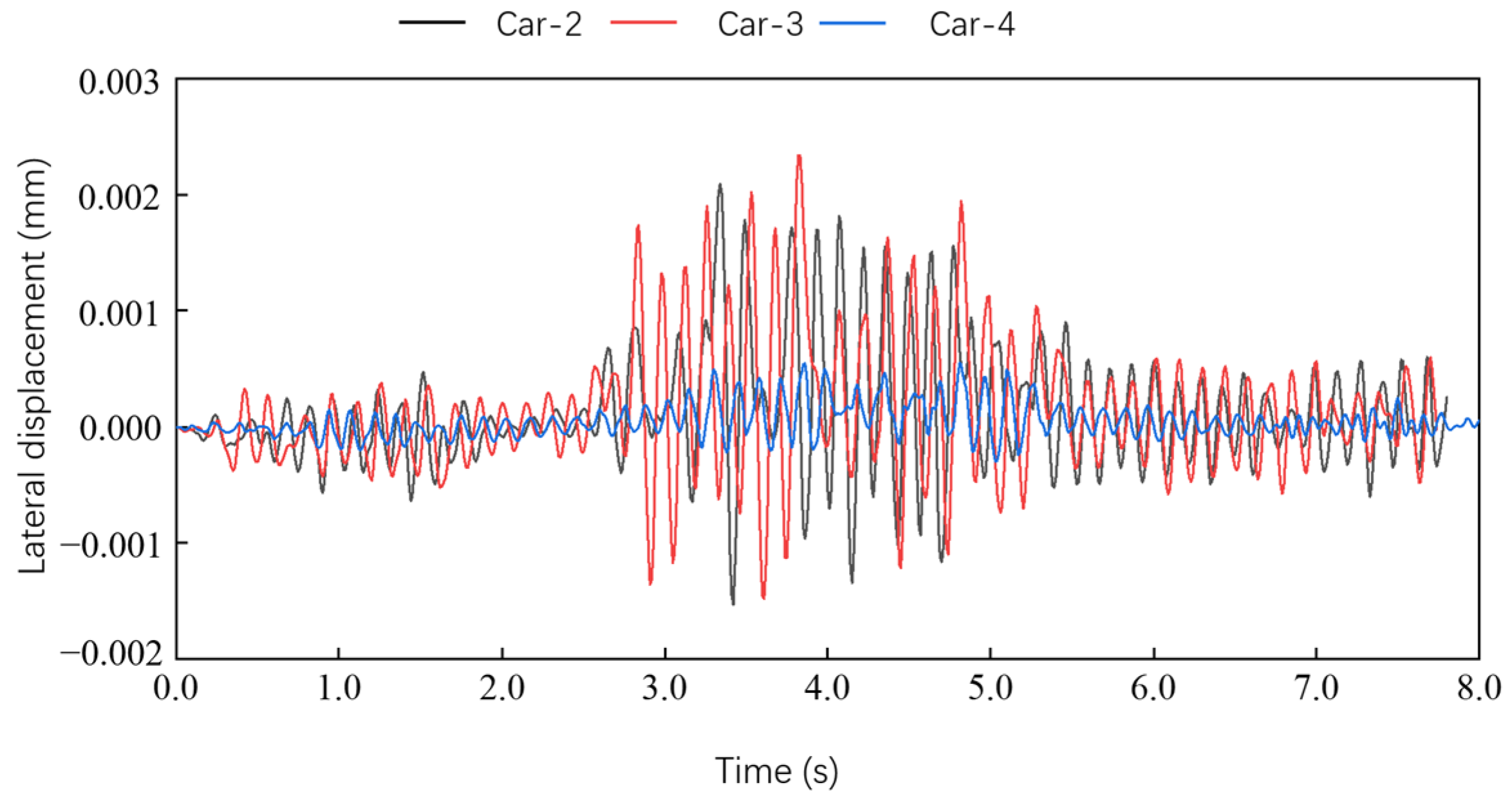
Different bridge constraints significantly affected bridges’ dynamic responses. Bridges’ vertical and torsional dynamic responses under rectangular coordinate constraints increased significantly compared to polar coordinates. As the axle weight of vehicles decreased, the mid-span vertical and torsional dynamic responses decreased while the lateral dynamic response gradually increased.

References

1. Zhou, L.; Liu, Z.W.; Yan, X.F.; Li, Q.F. Design Theory and Analysis Methods for Curved Girder Bridges; People’s Transportation Press: Beijing, China, 2018. [Google Scholar]
2. Liu, S.; De Corte, W.; Ding, H.; Taerwe, L. A comparison of the mechanical properties of curved box girders with corrugated steel webs to curved box girders with concrete webs. Adv. Struct. Eng. 2022, 25, 2103–2120. [Google Scholar] [CrossRef]
3. Zhu, L.; Wang, J.-J.; Li, M.-J.; Chen, C.; Wang, G.-M. Finite beam element with 22 DOF for curved composite box girders considering torsion, distortion, and biaxial slip. Arch. Civ. Mech. Eng. 2020, 20, 101. [Google Scholar] [CrossRef]
4. Nadi, A.; Raghebi, M. Finite element model of circularly curved Timoshenko beam for in-plane vibration analysis. FME Trans. 2021, 49, 615–626. [Google Scholar] [CrossRef]
5. Zhou, Y.; Zhang, K.; Miao, F.; Yang, P. Dynamic performance of straddle monorail curved girder bridge. Comput. Model. Eng. Sci. 2022, 130, 1669–1682. [Google Scholar] [CrossRef]
6. Eshkevari, S.S.; Matarazzo, T.J.; Pakzad, S.N. Simplified vehicle-bridge interaction for medium to long-span bridges subject to random traffic load. J. Civ. Struct. Health Monit. 2020, 10, 693–707. [Google Scholar] [CrossRef]
7. Liu, Y.; Yan, W.; Yin, X.; Wang, L.; Han, Y. Vibration analysis of the continuous beam bridge considering the action of jump impacting. Adv. Struct. Eng. 2022, 25, 2627–2640. [Google Scholar] [CrossRef]
8. Gara, F.; Nicoletti, V.; Carbonari, S.; Ragni, L.; Dall’asta, A. Dynamic monitoring of bridges during static load tests: Influence of the dynamics of trucks on the modal parameters of the bridge. J. Civ. Struct. Health Monit. 2020, 10, 197–217. [Google Scholar] [CrossRef]
9. Cantero, D.; Hester, D.; Brownjohn, J. Evolution of bridge frequencies and modes of vibration during truck passage. Eng. Struct. 2017, 152, 452–464. [Google Scholar] [CrossRef]
10. Zakeri, J.A.; Feizi, M.M.; Shadfar, M.; Naeimi, M. Sensitivity analysis on dynamic response of railway vehicle and ride index over curved bridges. Proc. Inst. Mech. Eng. Part K J. Multi-Body Dyn. 2017, 231, 266–277. [Google Scholar] [CrossRef]
11. Ma, Q.Q.; Zhang, J. Study on Vehicle-Bridge Coupled Vibration of Small-Radius-Curved Trough Girder Bridge. Bridge Constr. 2018, 48, 24–28. [Google Scholar]
12. Guo, F.; Cai, H.; Li, H.F. Impact coefficient analysis on long-span beam bridge. J. Vibroeng. 2021, 23, 436–448. [Google Scholar] [CrossRef]
13. Liu, S.; Yan, S.M.; Liu, C.J.; Wang, X. Analysis of Vehicle-Bridge Coupling Response of Curved CFST Composite Truss Bridge. Technol. Highw. Transp. 2023, 39, 89–98. [Google Scholar]
14. Zhou, R.-J.; Wang, Y.; Chen, H. Analysis of vehicle-bridge coupled vibration of long-span curved truss bridge in service. J. Vib. Eng. 2022, 35, 103–112. [Google Scholar]
15. Li, Z.; Li, Z.D.; Chen, D.H.; Xu, S.; Zhang, Y. Theoretical analysis and experimental study of vehicle-bridge coupled vibration for highway bridges. Arch. Appl. Mech. 2023, 94, 21–37. [Google Scholar] [CrossRef]
16. Shi, Y.; Fang, S.T.; Tian, Q.Y.; Chen, W. Spatial analysis of vehicle-bridge coupled vibration response between curved continuous rigid-frame bridge and motor vehicle. Appl. Mech. Mater. 2012, 1802, 2456–2461. [Google Scholar] [CrossRef]
17. Guo, F.; Cai, H.; Li, H.F. Impact coefficient analysis of curved box girder bridge based on vehicle-bridge coupling. Math. Probl. Eng. 2022, 2022, 8628479. [Google Scholar] [CrossRef]
18. Cao, H.T.; Chen, D.H.; Zhang, Y.S.; Wang, H.; Chen, H. Finite Element Analysis of Curved Beam Elements Employing Trigonometric Displacement Distribution Patterns. Buildings 2023, 13, 2239. [Google Scholar] [CrossRef]
19. Nallasivam, K.; Dutta, A.; Talukdar, S. Dynamic analysis of horizontally curved thin-walled box-girder bridge due to moving vehicle. Shock. Vib. 2007, 14, 65–84. [Google Scholar] [CrossRef]
20. Zhang, X.; Chen, E.L.; Li, L.Y.; Si, C. Development of the dynamic response of curved bridge deck pavement under vehicle-bridge interactions. Int. J. Struct. Stab. Dyn. 2022, 22, 1720–1735. [Google Scholar] [CrossRef]
21. Zeng, Q.Y.; Guo, X.R. Theory and Application of Vibration Analysis for Time-Varying System of Train-Bridge; China Railway Press: Beijing, China, 1999. [Google Scholar]
22. Luo, X.T. Dynamic Response Analysis of a Long Span Cable-Stayed Bridge Subjected to Automobiles. Master’s Thesis, Beijing Jiaotong University, Beijing, China, 2018. [Google Scholar]
23. Zong, Z.H.; Xue, C.; Yang, Z.G. Vehicle load model for highway bridges in Jiangsu province based on WIM. J. Southeast Univ. 2020, 50, 143–152. [Google Scholar]
Figure 1. Vehicle spatial vibration analysis model.
Applsci 14 02021 g001
Figure 2. (a) Cross section of the girder (unit: cm), (b) plan view of the curve bridge (unit: cm).
Applsci 14 02021 g002
Figure 3. Uniform moving spring-mass system acting on a simply supported girder.
Applsci 14 02021 g003
Figure 4. Comparison of the displacement time-history curves at mid-span.
Applsci 14 02021 g004
Figure 5. Comparison of the acceleration time-history curves at mid-span.
Applsci 14 02021 g005
Figure 6. Time-history curve of mid-span vertical displacement under different curvature radii.
Applsci 14 02021 g006
Figure 7. Time-history curve of mid-span vertical acceleration under different curvature radii.
Applsci 14 02021 g007
Figure 8. Time-history curve of mid-span torsional displacement under different curvature radii.
Applsci 14 02021 g008
Figure 9. Peak dynamic response of bridge mid-span under different curvature radii: (a) vertical displacement; (b) vertical acceleration; (c) torsional displacement.
Applsci 14 02021 g009
Figure 10. Mid-span vertical displacement under different constraints.
Applsci 14 02021 g010
Figure 11. Mid-span vertical acceleration curves under different constraints.
Applsci 14 02021 g011
Figure 12. Mid-span torsional displacement curves under different constraints.
Applsci 14 02021 g012
Figure 13. The mid-span vertical displacement curves under different vehicles.
Applsci 14 02021 g013
Figure 14. The mid-span vertical acceleration curves under different vehicles.
Applsci 14 02021 g014
Figure 15. The mid-span lateral displacement curves under different vehicles.
Applsci 14 02021 g015
Figure 16. The mid-span lateral acceleration curves under different vehicles.
Applsci 14 02021 g016
Figure 17. The mid-span torsional displacement curves under different vehicles.
Applsci 14 02021 g017
Figure 18. Mid-span dynamic response peaks of the bridge under different vehicle types: (a) vertical displacement peak; (b) vertical acceleration peak; (c) lateral displacement peak; (d) lateral acceleration peak; (e) and torsional displacement peak.
Applsci 14 02021 g018aApplsci 14 02021 g018b