Article

Digital-Twin-Based System for Foam Cleaning Robots in Spent Fuel Pools

School of Automation, Beijing Information Science and Technology University, Beijing 100101, China
*
Author to whom correspondence should be addressed.
Appl. Sci. 2024, 14(5), 2020; https://doi.org/10.3390/app14052020
Submission received: 19 January 2024 / Revised: 18 February 2024 / Accepted: 25 February 2024 / Published: 29 February 2024
(This article belongs to the Special Issue Intelligent Robotics: Design and Applications)

Abstract

:
This paper introduces a digital-twin-based system for foam cleaning robots in spent fuel pools, aiming to efficiently clean foam in spent fuel pools. The system adopts a four-layer architecture, including the physical entity layer, twin data layer, twin model layer, and application service layer. Initially, the robot was modeled in two dimensions, encompassing physical and kinematic aspects. Subsequently, data collection and fusion were carried out using laser radar and depth cameras, establishing a virtual model of the working scenario and mapping the physical entity to the digital twin model. Building upon this foundation, improvements were made in applying the full-coverage path planning algorithm by integrating a pure tracking algorithm, thereby enhancing the cleaning efficiency. Obstacle detection and localization were conducted using infrared and depth cameras positioned above the four corners of the spent fuel pool, with the digital twin platform transmitting coordinates to the robot for obstacle avoidance operations. Finally, comparative experiments were conducted on the robot’s full-coverage algorithm, along with simulation experiments on the robot’s position and motion direction. The experimental results indicated that this approach reduced the robot’s overall cleaning time and energy consumption. Furthermore, it enabled motion data detection for the digital twin robot, reducing the risk of collisions during the cleaning process and providing insights and directions for the intelligent development of foam cleaning robots.

1. Introduction

Cleaning robots can autonomously perform cleaning tasks in indoor or outdoor environments. They typically possess functionalities such as environmental recognition, path planning, autonomous navigation, intelligent obstacle avoidance, and automatic cleaning. Commercial applications of cleaning robots are widespread and can be found in apartments, hotels, shopping malls, public spaces, and outdoor areas like roads. With the introduction of concepts like “Industry 4.0” and the development guidelines outlined in “Made in China 2025”, cleaning robots are undergoing continuous transformation towards greater intelligence. Water cleaning robots are making significant strides in their development, to address complex application scenarios [1].
The term “spent fuel pool” refers to the storage pool where used nuclear fuel from a nuclear reactor is placed after removal. Its primary task is storing the used nuclear fuel safely while awaiting further processing [2,3]. In practical operations, factors such as activities within the pool, mechanical equipment wear, and airborne dust can lead to the generation of foam on the surface of the water of the spent fuel pool. Cleaning this foam is necessary for the spent fuel storage process and has been a persistent technological challenge. With the rise of intelligent manufacturing, cleaning robots have gained widespread application due to their environmental perception, decision-making, and motion control capabilities. Adopting cleaning robots for debris removal has become a trend, replacing traditional manual retrieval and fixed filtration circuits. However, conventional cleaning robots face challenges such as opaque motion data and significant accuracy deviations during operation, hindering their ability to meet cleaning requirements. Therefore, there is an urgent need to leverage new technologies and methods to facilitate the transformation of traditional cleaning robots towards intelligence.
A digital twin is an intelligent approach that integrates new sensing technologies, data collection technologies, virtual reality, 3D visualization, and intelligent human–machine interaction, and incorporates the concept of digital governance and interdisciplinary knowledge. The concept of digital twin was first proposed by Professor Grieves in 2003. Its core idea is to create a virtual digital representation that corresponds to objects or processes in the real world using digital technology [4]. Subsequently, many scholars at home and abroad have actively engaged in the research and practice of digital twin technology, achieving significant results. Tao Fei and others contemplated the ten major issues of digital twins, introduced the concept of a five-dimensional model, and provided theoretical foundations and ideas for applying digital twins in product design, technological applications, and lifecycle maintenance [5,6,7]. Li Hao and others systematically discussed the concept, structure, and operational mode of industrial digital twin systems by comparing different categories [8]. Stan Liliana and others established a digital twin robot working platform aimed at eliminating glitches. Wang Yan and others used a digital twin to establish a twin-body model of a gearbox, simulated the operational states of gearboxes under different conditions, and achieved precise fault diagnosis for gearboxes [9]. Söderberg affected the product production process using a digital twin, enabling real-time control and optimization of product production, and facilitating the transition from mass production to personalized customization [10]. Wei Yixiong, Guo Lei, and others proposed a real-time data-driven digital twin workshop system architecture and technical route. They achieved real-time visualization monitoring, health management, and intelligent workshop production status fault diagnosis by building a virtual simulation environment of the actual physical behavior and employing an event-responsive data management approach [11]. Many scholars have recognized the potential application of digital twin technology in robotics. MO et al. proposed the first robot-centric intelligent digital twin framework, Terra, to deploy robots in challenging environments, thereby achieving state monitoring and optimization of robots [12]. Stan Liliana and others established a digital twin robot working platform aimed at eliminating glitches. This platform achieved communication links between the robot and a virtual controller, presenting a novel approach to project-based intelligent robot manufacturing models and concepts such as information-physical systems, digitization, data collection, continuous monitoring, and intelligent solutions [13]. Wei Xinyu et al. combined digital twin technology to propose a surface-cleaning robot control system solution supporting robot path planning and motion control, effectively achieving the cleaning of charcoal surfaces [14]. Chancharoen, R et al. utilized digital twin technology to develop a collaborative painting robot that can substitute for human workers. The robot can simulate the entire process, and the feasibility of the solution was validated through experiments [15]. Zhu Zhiqiang designed and implemented a robot milling motion simulation and visual monitoring system based on a digital twin system framework. This system utilizes the Unity3D platform to construct a digital twin body of the robot, and they designed material removal algorithms based on grid deformation, established milling motion simulation models, and validated the effectiveness and timeliness of the system through experiments [16]. Farhadi A. et al. introduced a digital twin framework for robot drilling, achieving real-time visualization of drilling process parameters [17].
The above indicates that digital twinning can play a crucial role in the operation of robots [18]. However, most current research in the digital twin domain needs bidirectional data interaction capabilities for real-time mapping of robot operational processes. There still needs to be an improvement in achieving real-time synchronization. Moreover, the robot often needs better processing capabilities when confronted with complex environmental conditions, due to inherent power and computational capacity limitations. Consequently, this paper addressed the challenges posed by a fuel-depleted pool foam cleaning robot by establishing a digital twin model within the ROS environment. Through research on simulating the cleaning activities of the robot, we applied the pure tracking algorithm concept to refine a complete coverage path planning algorithm, thereby enhancing the smoothness of its movements. Additionally, real-time obstacle detection and localization were facilitated using the digital twin system platform to prevent collisions with obstacles lying beyond the existing map during the cleaning process. Subsequently, the obstacle positions were transmitted to the robot, aiding in its obstacle avoidance maneuvers. Lastly, building upon this foundation, we validated the accuracy of the data and the synchronization consistency between virtual and real robots by examining the positional coordinates and movement directions of both entities at four random time points.

2. Digital Twin Technology Architecture for Surface Robots

As shown in Figure 1, leveraging digital twin technology and integrating the workflow of the foam cleaning robot, this study designed a digital twin technology architecture specifically for the foam cleaning robot in spent fuel pools. The architecture is primarily divided into four parts: the physical entity layer, twin data layer, twin model layer, and application service layer. The robot and the digital twin system exhibited excellent stability and safety with this modular four-layer design.
Assuming that the digital twin framework (DFT) represents the digital twin framework, and ::= signifies being defined as, where PEL stands for the physical entity layer, TDL represents the twin data layer, TML represents the twin model layer, and ASL means the application service layer, the architecture is depicted as shown in Equation (1).
D F T : : = P E L , T D L , T M L , A S L

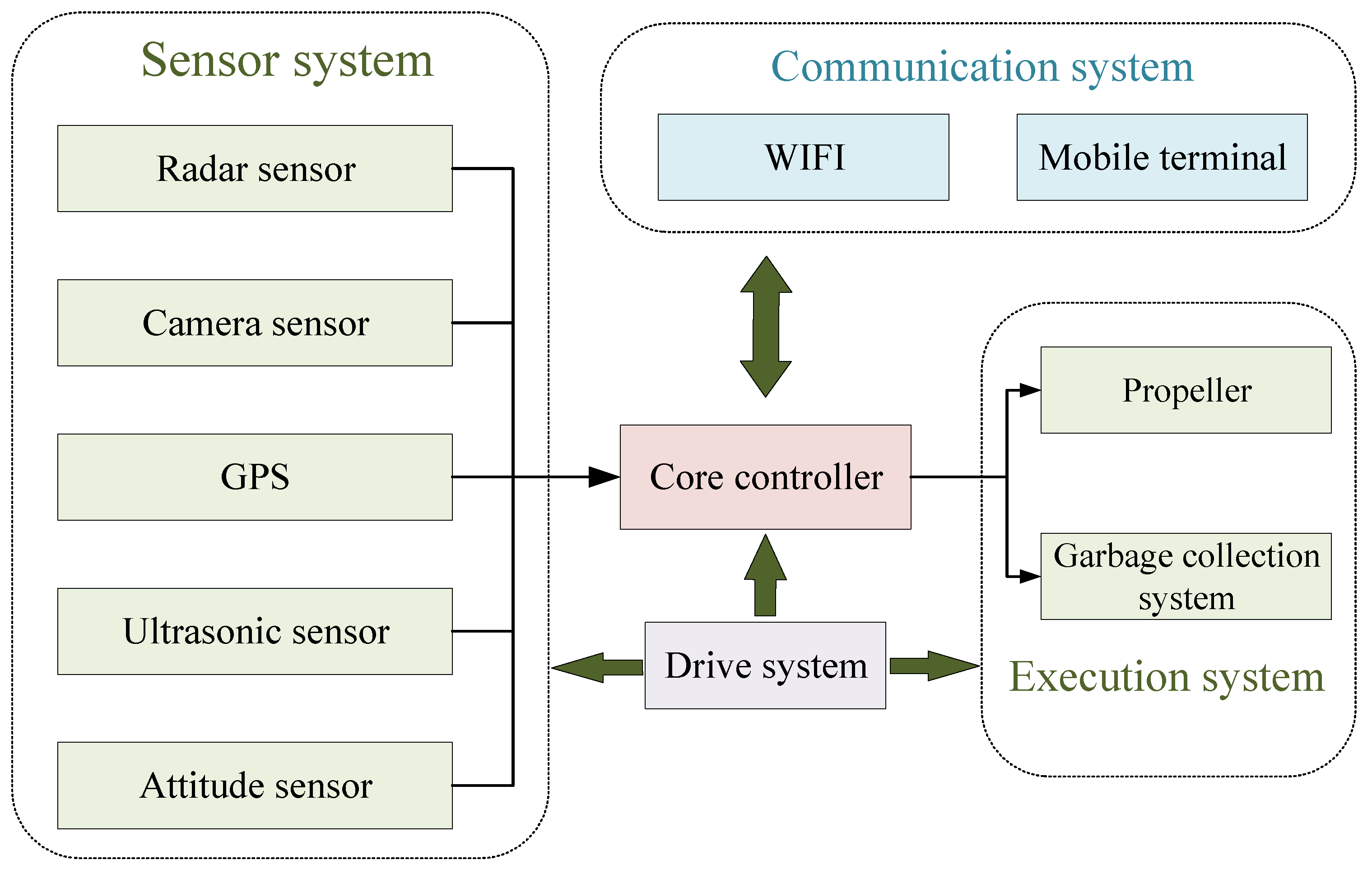
2.1. Physical Entity Layer (PEL)

The PEL is the foundational framework of the digital twin system, primarily composed of scene devices in physical space. This includes the entities of both the robot and the spent fuel pool. Functionally, it can be divided into three modules: the network module, the perception module, and the control and execution module. The devices at this level constitute the actual operational units of the digital twin system. They receive instructions from the digital twin system, execute tasks accordingly, and directly interact with the natural environment, making them the interface for interaction between the system and its physical surroundings.

2.2. Twin Data Layer (TWL)

The TWL serves as the foundation of the digital twin system, responsible for managing and processing physical data, acting as a bridge between the physical and virtual spaces, and allowing their mutual influence. Its functions primarily include classifying, analyzing, and integrating real-time physical data from sensors such as lidar, depth cameras, and ultrasound arrays. This encompasses both physical space data and virtual space data, with physical space data including the robot’s position and orientation, the positions of walls and obstacles, and the cleaning area. Virtual space data include the simulation and decision data. Finally, these data are transmitted to the application service layer for further processing.

2.3. Twin Model Layer (TML)

The TML is the digital twin body that integrates the physical entity and twin data layers. Acquiring detailed data from the data layer enables comprehensive modeling and simulation of the surface robot, encompassing both the robot model and the spent fuel pool environment model. This layer includes geometric modeling, physical modeling, behavioral modeling, and rule modeling, ensuring that the TML accurately reflects and simulates the robot’s motion, interaction, and response in the actual spent fuel pool environment.

2.4. Application Service Layer (ASL)

The ASL is primarily designed to meet the application requirements of DFT, utilizing the rich data provided by the twin data layer, including initial positions and target constraints. It engages in virtual scene construction, model driving, and robot motion. The system uses these data to accomplish tasks such as obstacle avoidance, complete coverage path planning, collision detection, and viewpoint switching. Additionally, the ASL offers visualization services, presenting the robot’s motion state and path to the user accurately and intuitively.

3. Implementation of the Digital Twin System for the Foam Cleaning Robot in Spent Fuel Pools

3.1. Establishment of the Physical Model for Robots

Establishing a digitized virtual model consistent with physical entities is crucial for digital twin modeling. This paper, using the characteristics of the digital twin system for the foam cleaning robot in spent fuel pools, presents the specific modeling process as follows:
(1) Utilizing SolidWorks 2022, a three-dimensional model of the robot’s appearance and structure was established. This encompasses the overall shape of the robot (catamaran), propellers, and foam collection device. Subsequently, the model was exported as an STL file, which was converted into COLLADA format. Throughout this process, the geometric information of the robot model was preserved, allowing effective loading and utilization within the ROS system.The overall structure diagram of the robot system is as shown in Figure 2.
(2) Based on the actual shape, color, dimensions, mass, and inertia parameters of the robot, a URDF file was written to provide a detailed description of the robot’s structure and characteristics. Among these, the robots could be approximated as dual-body ship models, with maximum lengths and widths measuring 70 cm, maximum height of 40 cm, and a mass of 20 kg. The URDF file encompasses definitions for the robot’s joints, sensors, and links, and specifies their relationships and constraints. This file enabled the ROS system to comprehend and simulate the physical attributes of the robot, providing an accurate robot model for subsequent tasks such as simulation, control, obstacle avoidance, and path planning. Figure 3 illustrates the schematic of the robot’s structure, Table 1 lists the inventory of robot components, Figure 4 depicts the physical representation of the robot and Figure 5 shows the controller circuit diagram.
(3) In the URDF file, the sensors such as the laser rangefinder, depth camera, ultrasonic sensor, and attitude sensor are configured. This configuration imparts the robot with the capability to perceive and receive external information, enabling the robot to simulate the real-world perception process. Consequently, this provides an accurate perceptual foundation for robot navigation and path planning.
(4) After completing digital modeling, the URDF file was loaded into ROS, utilizing RViz for visualization. This allowed an intuitive observation of the robot’s appearance, posture, and feedback from sensor data. It further facilitated simulation and control of the robot within the ROS environment.

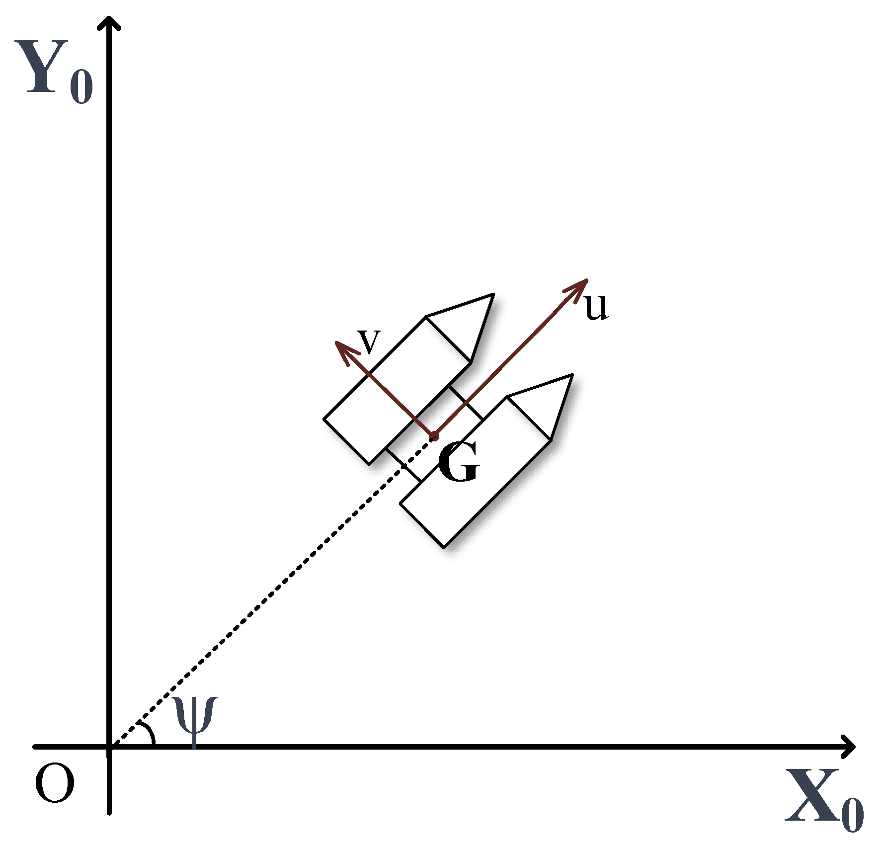
3.2. Establishment of the Robot Motion Model

The motion model of the robot serves as the fundamental basis and core concern for implementing robot motion control. In this paper, the robot adopted the form of a catamaran, and the MMG model was utilized to establish a motion model of the catamaran, employing mathematical equations to describe its motion process.
To determine the position and orientation of the robot during surface movement, it was necessary to establish a coordinate system suitable for its motion control. Cartesian coordinates are widely used in the study of robot motion, including both fixed coordinate systems and moving coordinate systems. This paper neglected the robot’s heaving, pitching, and rolling motions. The six degrees of freedom were simplified into a plane motion state with only three degrees of freedom. Based on the above, a coordinate system for the planar motion of the surface robot was established. A schematic diagram of the planar motion of the surface robot is shown in Figure 6.
X 0 = X cos ψ Y sin ψ Y 0 = X sin ψ + Y cos ψ N 0 = N Y x d
x ˙ G = u cos ψ v sin ψ y ˙ G = u sin ψ + v cos ψ ψ ˙ = r
In Equations (2) and (3), u and v represent the longitudinal and lateral velocities of the robot, respectively, while r is the rate of change of the robot’s heading angle ψ concerning time. X 0 , Y 0 , and N 0 denote the external forces and moments acting on the robot in the inertial coordinate system. X, Y, and N represent the external forces and moments acting on the robot in the body-fixed coordinate system. x G and y G are the coordinates of the robot’s center of gravity G, x d is the coordinate value of the robot’s center in the body-fixed coordinate axis, and Y x d is a correction term.
The actual motion equations of the robot can be expressed as follows:
X 0 = m x ¨ G Y 0 = m y ¨ G N 0 = I z ψ ¨
In Equation (4), m represents the mass of the robot, and I z represents the mass moment of inertia of the robot body about the vertical axis passing through the center of gravity.
Taking the time derivative of Equation (3), we obtain
x ¨ G = u ˙ cos ψ v ˙ sin ψ u sin ψ + v cos ψ ψ ˙ y ¨ G = u ˙ sin ψ + v ˙ cos ψ + u cos ψ v sin ψ ψ ˙ ψ ¨ = r ˙
Substituting Equation (4) into Equation (5), we obtain
X 0 = m u ˙ v ψ ˙ cos ψ m v ˙ + u ψ ˙ sin ψ Y 0 = m u ˙ v ψ ˙ sin ψ + m v ˙ + u ψ ˙ cos ψ N 0 = I z r ˙
Combining and simplifying Equations (2) and (6), the motion model of the robot in the body-fixed coordinate system is obtained as follows:
X = m u ˙ v r Y = m v ˙ + u r I z r ˙ = N Y x d
Following the modeling concept of the MMG separation model [19], the external forces and moments acting on the robot are represented as follows:
X = X H + X P + X W + X C Y = Y H + Y P + Y W + Y C N = N H + N P + N W + N C
In these Equations, H represents the robot body, P represents the propeller, W represents the wind, and C represents the current.
Combining and simplifying Equations (7) and (8), the motion model of the surface robot with three degrees of freedom is obtained as follows:
m u ˙ v r = X H + X P + X W + X C m v ˙ + u r = Y H + Y P + Y W + Y C I z r ˙ = N H + N P + N W + N C Y x d

3.3. Construction of the Working Scenario for the Cleaning Robot

The construction of the working scenario formed the foundation for the successful operation of the robot. In constructing the scenario, this paper integrated a laser rangefinder and depth camera through sensor fusion in the ROS environment [20]. Multiple sensors were utilized to provide rich environmental information, and data fusion was employed to achieve complementary benefits from the sensors, thereby reducing the measurement error and enhancing the robot’s robustness.The workflow for constructing the work scene map is shown in Figure 7.
The laser radar used in this study was the RPLIDAR S2, capable of measuring distances ranging from 0.05 to 30 m with an accuracy of ± 30 mm. It has a ranging resolution of 13 mm, a sampling frequency of 32 kHz, and a scanning frequency of 10 Hz. The depth camera employed was an Astra Pro Plus, with a working range of 0.6 to 8 m and an accuracy of 1 m ± 3 mm. It operates at a frame rate of 30 fps with a horizontal field of view of 58.4 ° and a vertical field of view of 45.8 ° . The resolution is 640 × 480 , and the operational temperature range is 10 to 40 degrees Celsius.

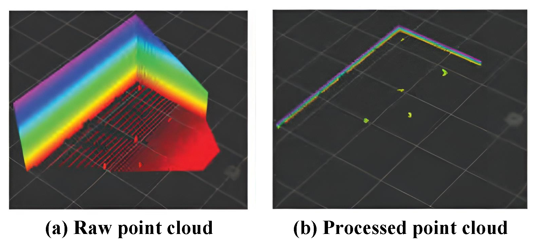
3.3.1. Processing of Depth Camera Point Clouds

The environment point cloud published by the depth camera contained many redundant points. In the context of this paper, where the robot could be approximated as a ground robot, excessively high walls and ground points did not contribute to obstacle information for mapping. Therefore, it was necessary to filter out these points. As shown in Figure 8, this is the process diagram for depth camera point cloud processing.
First, downsampling was applied to the point cloud produced by the depth camera. The point cloud was then converted into a format that the PCL library could process. Voxel filtering was performed to filter the point cloud, significantly reducing the number of points, while preserving the shape features. Subsequently, a height threshold was set to remove excessively high points, retaining obstacle points on the ground. Finally, ground points were removed using the standard vector method. The average vector for each point was calculated using the principal component analysis method for a given point cloud data. The average vector was considered as the plane normal vector, and by fitting the point cloud data to the plane model, the plane equation was obtained as A x + B y + C z + D = 0 , where A , B , C is the plane average vector, and x , y , z is the coordinates of the point. Each point’s coordinates were substituted into the plane equation, and the points that satisfied the equation were considered ground points and were removed from the point cloud. In Figure 9, both the raw point cloud data from the depth camera and the processed point cloud data are presented.

3.3.2. Sensor Data Fusion

The information obtained by the depth camera and the two-dimensional laser rangefinder differed in their representation. The mapping relationship between the point cloud and image data was obtained using the rotational and translational transformation relationship. This enabled data transformation into the same coordinate system for further processing.
Figure 10 shows the coordinate relationship between laser radar and depth camera. In Figure 10, the detected object has coordinates m D x d , y d , z d in the depth camera coordinate system, m L x l , y l , z l in the laser rangefinder coordinate system, and projection coordinates m ( u , v ) in the image coordinate system. For the depth camera, the collected information of point m includes the projection coordinates m ( u , v ) and the corresponding depth information z c . The laser rangefinder scanned and obtained the distance ρ and angle α between the radar and the object. Here, α represents the angle between the detected object and the O L Z L axis. Based on the geometric relationship between these two coordinate systems, the transformation relationship of the detected object between the two coordinate systems could be derived as follows:
x c y c z c = R T 0 T 1 x l y l z l
In Equation (10), R represents the rotation matrix, and T represents the translation matrix. m is the projection of the detected object on the image plane. In the depth camera coordinate system, the relationship between the depth information and projection coordinates is
z c u v 1 = f x 0 q x 0 0 f y q y 0 0 0 1 0 x c y c z c
In Equation (11), f x and f y represent the focal lengths on the X and Y axes, while q x and q y represent the baseline points on the X and Y axes. f x , f y , q x , and q y are intrinsic parameters of the camera. According to the above formula, the data of the detected object collected by the depth camera could be transformed into the laser rangefinder coordinate system. The transformation relationship between them is
z c u v 1 = f x 0 q x 0 0 f y q y 0 0 0 1 0 R T 0 1 x l y l z l
During the scanning process, the laser rangefinder adopted a polar coordinate expression. The relationship between the information collected by the laser rangefinder about the detected object in its coordinate system is
x l = ρ sin α z l = ρ cos α
It was ensured that the center points of the depth camera and laser rangefinder lay on the same axis, with the height difference between them denoted as δ . From the above formulas, the transformation relationship between the depth camera information and laser rangefinder information could be derived as:
z c u v 1 = f x 0 q x 0 0 f y q y 0 0 0 1 0 R T 0 1 ρ sin α h ρ cos α
By substituting the measured depth camera data and laser rangefinder data into the Equation (14), the rotation matrix and translation matrix in the system of linear equations could be determined. This completes the calibration to transform depth camera data into pseudo-laser rangefinder data. After the joint calibration of the sensors, the point clouds from both sensors were fused in the laser rangefinder coordinate system. The position coordinates of the fused points are denoted as m F = m D , m L , where m D represents the coordinates of the pseudo-laser rangefinder data from the depth camera, and m L represents the coordinates of the laser rangefinder data.

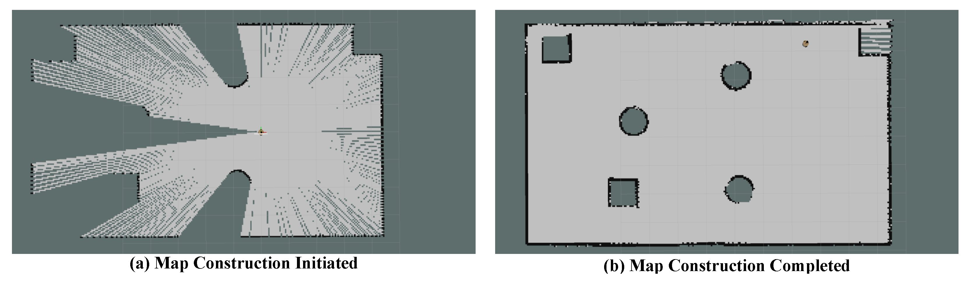
3.3.3. Construction of the Scene Map

After merging the two sets of point clouds, the combined point cloud was input into the Cartographer algorithm to complete the construction of a two-dimensional plane map [21]. The map construction involved two main steps: local submap construction and global loop closure optimization. In this process, a submap was defined as a frame of the merged point cloud, and loop closure detection was based on the entire submap.
Upon obtaining a frame of the merged point cloud, it was inserted into the optimal position of the submap. This process involved creating a grid submap and building a camera pose graph. Subsequently, the constructed grid submap was added to the loop closure detection queue. Suppose the estimated pose of the current point cloud is closest to the pose of a point cloud in the loop closure detection queue. In that case, a loop closure constraint is added to the corresponding position in the pose graph to help eliminate cumulative errors in local mapping.
Finally, loop closure optimization was performed between sub-maps to ensure high-precision consistency in the map’s local and global aspects. This optimization process involved adjustments between sub-maps, further enhancing the accuracy and completeness of the map and providing a reliable foundation for path planning for the robot in the spent fuel pool. Figure 11 depicts the process of scene map construction.

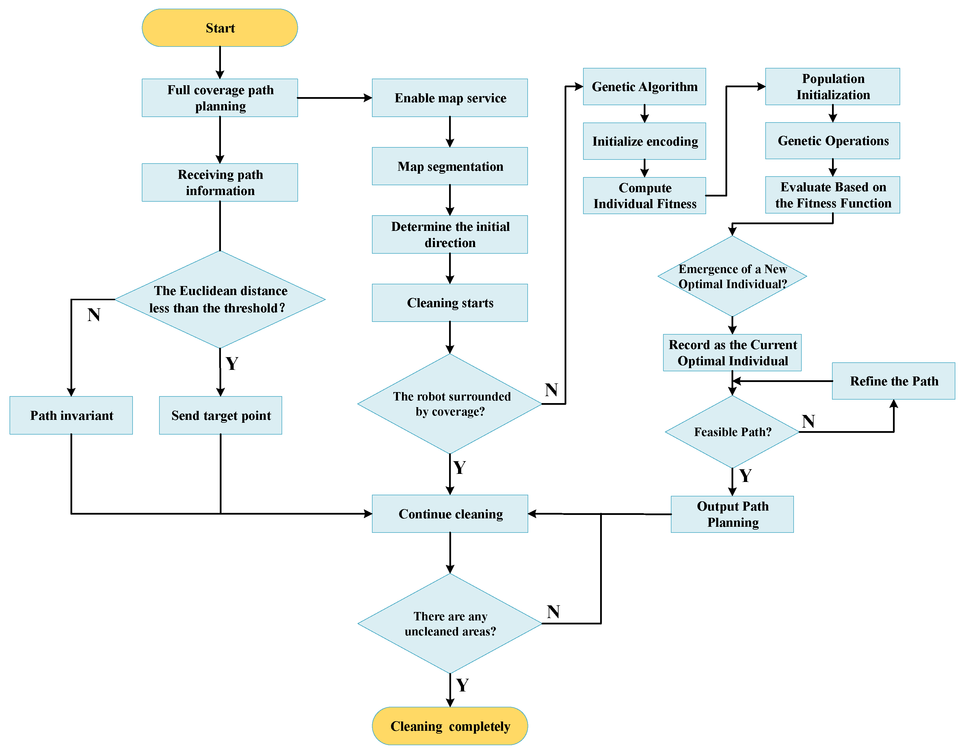
4. Digital Twin Collaborative Full-Coverage Path Planning Method

4.1. Construction of the Objective Function

The robot must traverse the entire environment with as few steps as possible, while autonomously avoiding obstacles on the map. Meanwhile, energy consumption is also crucial, to ensure the robot can successfully complete the task. The paper defines the following evaluation functions to analyze the algorithm’s performance. This evaluation function is divided into three parts:
(1) Site Coverage: In this paper, let S a represent the already covered area, S represent the total area of the working environment, and S o represent the area covered by obstacles. Therefore, the coverage rate r of the full-coverage path planning is calculated as r = S a S S o .
(2) Energy Consumption: This paper established an energy consumption model for the robot. Let t s be the time for the robot to move in a straight line, t t be the time for the robot to turn, and t r be the time the robot is stationary on the water. The power for turning is denoted as P t , and the power of the robot’s control module is marked as P c . The energy consumed by the control module is denoted as E c .
Simplifying the force relationship of the robot in the spent fuel pool, the paper focused only on the traction force F generated by the robot’s movement in the water and the resistance f experienced by the robot. Additionally, assuming the robot moves at a constant speed v, the energy consumption E m of the robot’s motion module can be expressed as
E c = P c ( t s + t t + t r )
E m = ( F f ) v t s + P t t t
Let the total energy consumption of the robot be E t t , then the final energy consumption model for the robot performing the cleaning task is given by
E t t = E c + E m = F f v + P c t s + P t + P c t t + P c t r

4.2. Selection and Improvement of the Full-Coverage Path Planning Algorithm

The path planning algorithm in this paper can be broadly divided into three main parts:
(1) Behavior-based coverage for full coverage path planning:
In the process of full coverage path planning for the robot, considering the relatively stable environment of the fuel-depleted pool and aiming to enhance the simplicity and adaptability of the algorithm, as well as taking into account the computational limitations of the robot itself and the goal of minimizing robot energy consumption to the greatest extent possible, this paper adopted behavior-based coverage. The basic process of behavior-based coverage is as follows: (a) Initialization: Set the starting point of the initial path in advance. (b) Consider the robot’s size sufficiently, and partition the map into appropriately sized grids. (c) The system generates the robot’s motion path and determines the initial direction. Upon determining the path, obstacles are detected, and if the robot detects an obstacle, the path is discarded; otherwise, it is considered a candidate path. (d) From all the candidate paths, select the path with the shortest length as the final path. (e) In actual movement, the robot will move linearly in the environment along the path. When an obstacle is detected, it will rotate clockwise 90° to achieve an S-shaped movement. Suppose the area around the robot has been completely covered. In that case, the path is determined by applying a genetic algorithm [22,23] from the current robot position to the endpoint of the uncovered area. This process is repeated until the entire cleaning task has been completed.
(2) Improvement with Pure Tracking Algorithm:
However, the above algorithm has some limitations in practical applications. This is mainly because the planned path after completion only includes the central positions of the map segmentation, with each point being separated by the size of only one cleaning robot. Additionally, the robot only sends the next path planning point when it has reached a certain determined point, which may result in frequent starts and stops during task execution, significantly increasing the hover time of the robot and thus reducing cleaning efficiency. To address this issue, an improvement was made to the complete coverage path planning algorithm by integrating the pure tracking algorithm [24]. The core objective of the pure tracking algorithm is to achieve precise tracking and control of the robot to the target point, ensuring that the robot can move along the expected trajectory and ultimately reach the target position. Its main idea is to dynamically generate and adjust the robot’s motion trajectory in real time based on the current state of the robot, the position of the target point, and predefined control strategies, enabling stable tracking of the target point. The specific changes made in this paper were as follows: During the robot’s movement, the next path planning point is no longer only sent when the target point is reached. Instead, it is dynamically generated based on the current position and state of the robot. The Euclidean distance between the current robot position and the set target point is calculated based on the feedback pose data from the current robot odometer. The system determines whether the current distance is less than a set threshold at each moment. If it indicates that the robot is close to the target point, the system can immediately send the next path planning point. If it is greater than the threshold, the current motion continues. This allows the robot to move more smoothly during task execution, avoiding frequent stops and achieving a more continuous and efficient motion trajectory. Consequently, this significantly improves the cleaning efficiency and enhances the practicality and benefits of the robot in real-world applications.
(3) Local Path Planning Using Genetic Algorithm:
As mentioned in (1), if the area around the robot has been completely covered, the problem is transformed into a local path planning problem between the starting point and the target point, with the current robot position as the starting point and the uncleared area as the target point. In this case, a genetic algorithm was adopted in this paper to address this issue.
A genetic algorithm is a computational model that simulates Darwinian biological evolution theory to search for the optimal solution to a problem. It starts with a population representing a set of possible solutions to the problem, consisting of several individuals encoded with genes. Each individual represents an entity with characteristics internally represented as chromosomes containing a set of genes. Therefore, encoding from data features to genes is needed.
During the evolution process of genetic algorithms, increasingly excellent approximate solutions are generated, generation by generation, based on the principles of survival of the fittest and natural selection. In each generation, individuals are selected based on their fitness, and genetic operators such as crossover and mutation are applied to produce new solution populations. This process leads to the natural evolution of the population into offspring populations that are better adapted to the environment. After multiple generations of evolution, the best individual in the final population, decoded from genes, can serve as an approximate optimal solution to the problem.
A genetic algorithm mainly involves operations such as encoding, crossover, and mutation of genes, which can be implemented in various ways. This section mainly adopts a path-based encoding method, crossover operation based on partial matching, and mutation operation based on exchange.
Figure 12 and Figure 13 respectively depict the flowchart of the robot cleaning process and the robot cleaning operation.

5. Obstacle Detection and Localization

To facilitate human operations, temporary devices such as floating platforms, floating barriers, and buoys may be intermittently placed on the surface of the fuel-depleted pool. These devices, potentially positioned along pre-planned operational routes, pose a safety risk, as they are prone to collisions with the robot. Due to the limited computational capacity of the robot itself and the need to minimize its energy consumption, obstacle detection, and localization were conducted using a digital twin system platform. This platform provided effective feedback regarding obstacle positions relative to the robot’s status. Initially, RGB images and depth maps of the pool environment were obtained through infrared and depth cameras positioned above the four corners of the pool. Subsequently, an obstacle detection algorithm based on YOLOv5 was employed to identify obstacles in the RGB images and obtain pixel coordinates of the obstacle’s location. The three-dimensional coordinates and depth information of the obstacle’s location in the camera coordinate system were computed by combining depth information. Following a target transformation, the absolute coordinates of the impediment to the water surface coordinate system were derived. These coordinate data were then transmitted to the robot, enabling it to autonomously detect, locate, and navigate around obstacles in the spent fuel pool.

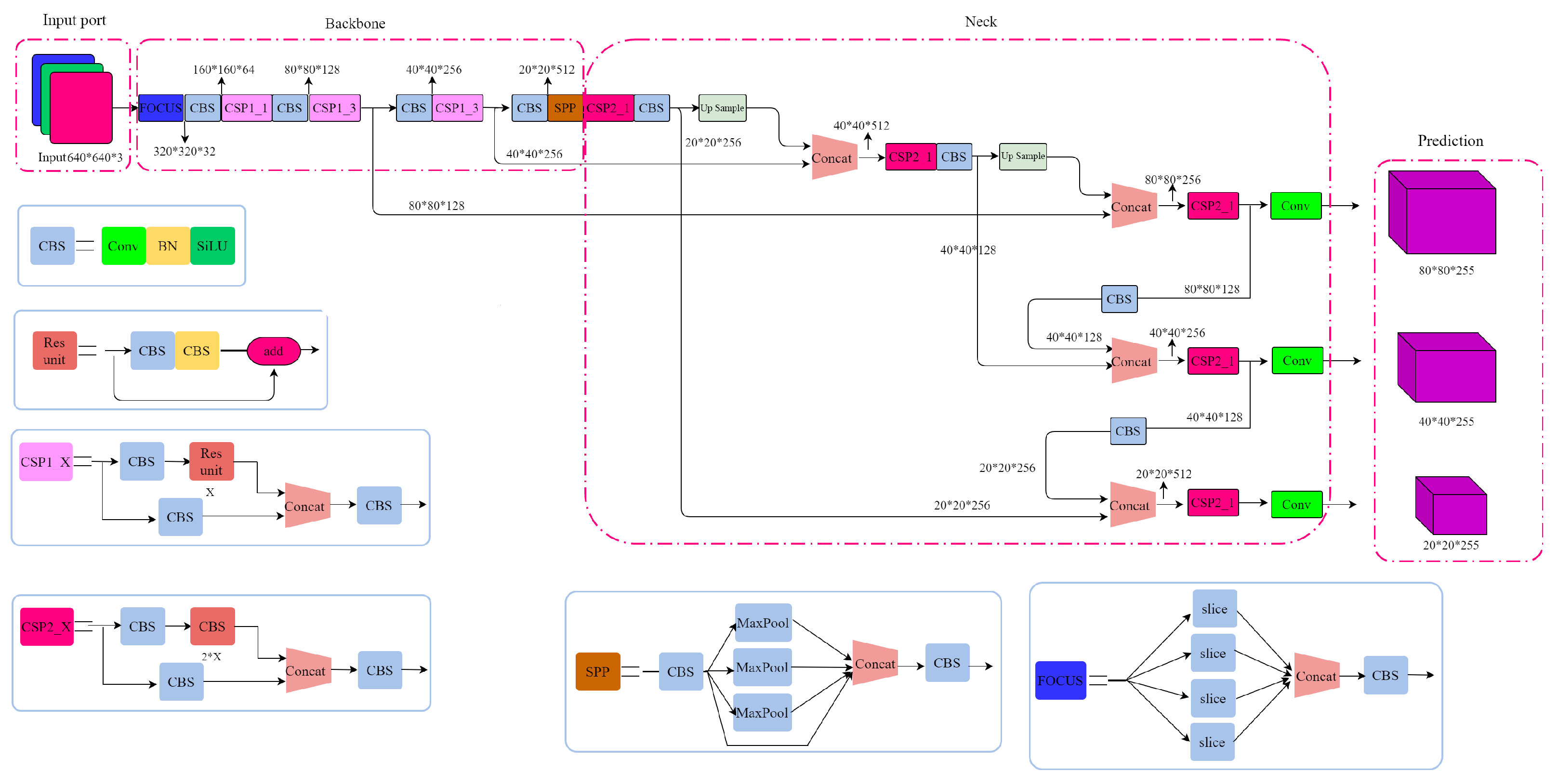
5.1. Object Detection Based on YOLOv5

YOLOv5 (You Only Look Once version 5) is a real-time object detection algorithm renowned for its efficient, rapid, and accurate performance. The network architecture of this algorithm can be divided into four main components: the input layer, backbone network, neck, and predictions. Through the collaborative interaction of these four crucial components, YOLOv5 achieves rapid object detection, while maintaining a high accuracy, showcasing its excellence in real-time scenarios and complex environments. The YOLOv5 network architecture diagram is shown in Figure 14.
(1) Input Layer: Images are initially fed into the YOLOv5 network. This algorithm supports various input sizes, allowing users to balance speed and precision. Users can adjust the algorithm’s performance according to specific requirements by choosing different input sizes, better adapting it to various application scenarios.
(2) Backbone Network: The backbone network extracts features from the input images. YOLOv5 adopts CSPNet (cross-stage hierarchical network) as its backbone, enhancing its ability to capture hierarchical information. This improves its discriminatory power for detecting targets, extracting local and global features from the images. This ensures that YOLOv5 can more accurately represent the content of images in object detection tasks, thereby enhancing overall performance.
(3) Neck: The neck network fuses multi-scale features from the backbone network. YOLOv5 employs PANet (path aggregation network) as its neck network, primarily designed to connect feature maps of different scales. This enhances the model’s understanding and discriminatory ability towards targets, improving object detection accuracy.
(4) Prediction: The prediction component is responsible for predicting targets based on the output feature maps, including the bounding boxes, categories, and confidence scores of the targets. In this stage, YOLOv5 employs the mechanism of anchor boxes and conducts target predictions based on the scale of the feature maps. This effectively identifies and locates targets within the images.

5.2. Obstacle Coordinate Localization

Upon obtaining obstacle pixels from the target detection process, denoted as P, the point P is translated into the image coordinate system. Subsequently, the localization point P is mapped to three-dimensional space using a projection transformation. The final transformation relationship between the pixel coordinate system and the camera coordinate system is as follows:
Z c u v 1 = f x 0 u 0 0 f y v 0 0 0 1 X c Y c Z c
where u , v represents the two-dimensional location point of the obstacle in the pixel coordinate system, Z c is obtained from the depth camera, and f x , f y , u 0 , v 0 represents the intrinsic parameters of the depth camera, which are factory-calibrated by default. The three-dimensional coordinates of the obstacle localization point in the camera coordinate system can be solved using Equation (18) (assuming Z c = 0 by default).
X c = Z c u u 0 f x Y c = Z c v v 0 f y Z c = 0
As the aquatic robot operates in the water surface coordinate system along the planned route, local adjustments to the global path are necessary when obstacles are detected. To facilitate obstacle avoidance path planning, the obstacle information in the camera coordinate system needed to be transformed into a water surface coordinate system. This ensures that the position information of obstacles and the localization information of the aquatic robot are described in the same coordinate system.
X w Y w Z w 1 = R T 0 1 1 X c Y c Z c 1
where X w , Y w , Z w represents the coordinates in the water surface robot coordinate system, R is the product of the rotation matrices in the X , Y , Z directions, and T is the translation matrix.

5.3. Obstacle Avoidance Operations

After obstacle detection and target localization, the obtained position coordinates are transmitted to the robot, allowing it to quickly assess whether obstacles affect its standard navigation on the current path. When obstacles are detected on or near the path and hinder the robot’s standard navigation, appropriate obstacle avoidance measures are taken.
Furthermore, ultrasonic sensors are employed for obstacle avoidance if the visual system is affected by lighting conditions or obstruction. In this study, the HC-SR04 ultrasonic module was utilized, with a range of 0.02–4 m, an accuracy of ± 3 mm, and an operating temperature range of 0–50.
The principle of ultrasonic sensor ranging relies on the speed of sound propagation in the air, calculating the distance information of obstacles by measuring the time interval between the moment the source sound wave is transmitted and the moment the echo signal is received, as expressed in Equation (21).
S = 1 2 T 340 m / s
In Equation (21), S represents the distance between the sensor and the obstacle, and T denotes the echo duration, the duration of the signal level. Based on the distance obtained from Equation (21), and with a set distance threshold of 3 m, the robot will rotate clockwise by 90 degrees to continue its cleaning operation when the distance is less than this threshold.
In conclusion, the combination of visual and ultrasonic obstacle avoidance could provide robust obstacle avoidance capabilities, ensuring that the cleaning robot could navigate through complex environments effectively.

6. Experimental Validation and Analysis

To validate the feasibility of the methods proposed in this paper, the experimental system consisted of a local and remote end. The local end comprised the robot, spent fuel pool environment, laser radar, depth camera, etc. The remote end employed a high-performance computer with an Intel i7-7800X processor, 16GiB RAM, and RTX3090Ti graphics card in the experiment. Digital twin modeling was conducted in the ROS system to establish a digital twin model of the robot and its working environment.

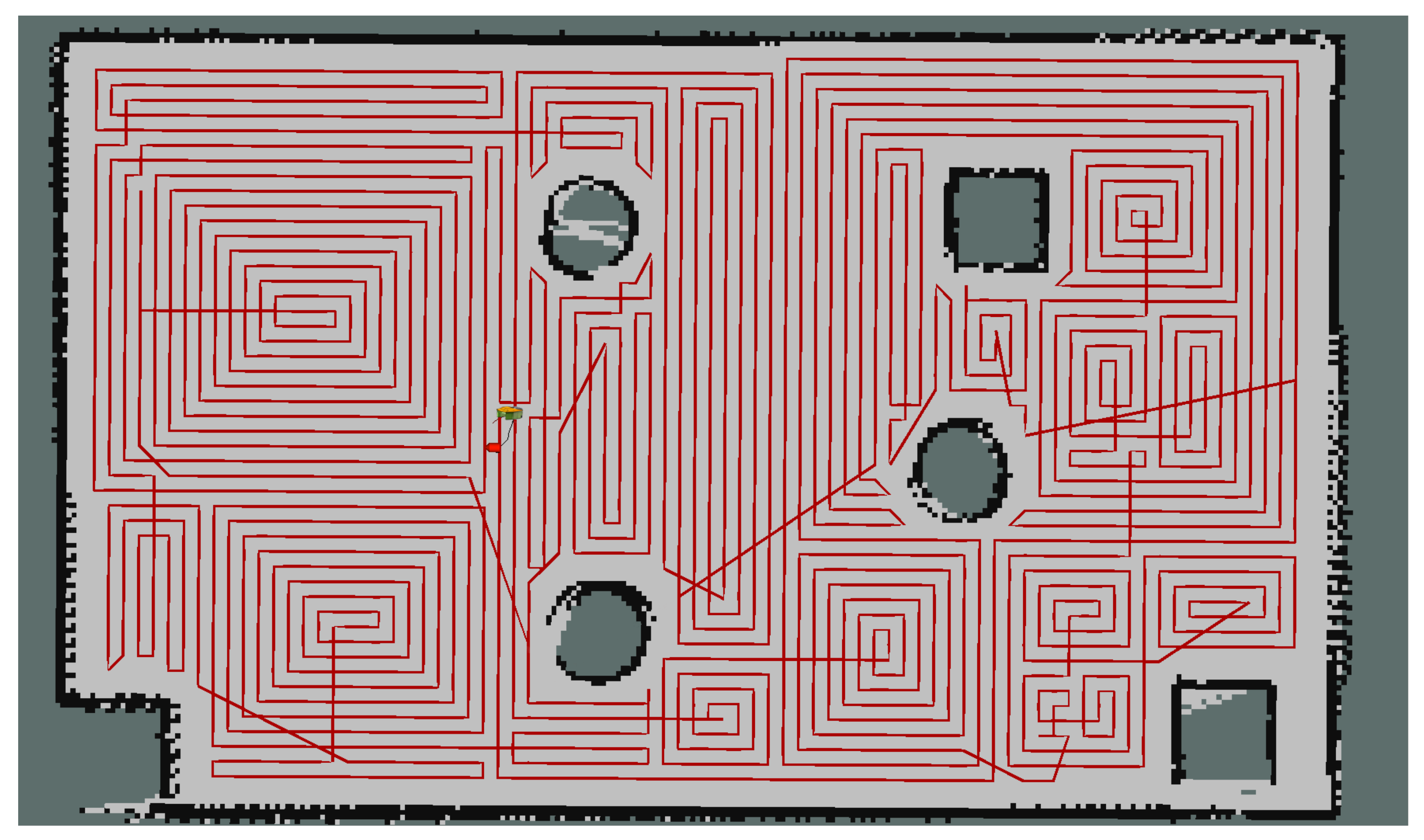
6.1. Comparative Evaluation of the Performance of the Improved Full-Coverage Path Planning Method

The resistance between the robot and the water surface was an essential parameter in the experimental evaluation. Due to the complexity of calculating the resistance formula, this study aimed to obtain the resistance value through experimentation. First, a force sensor was installed on the robot body, propelled forward at a constant velocity of v = 1 m/s. During this process, the force sensor experienced a corresponding force, converted into an electrical signal output. Subsequently, the output data of the force sensor were recorded and analyzed, resulting in a measured resistance between the robot and the water surface of approximately f = 65 N.
The parameters for the robot were set as follows: the resistance between the water surface and the robot was approximately f = 65 N, the constant velocity of the robot along the water surface was v = 1 m/s the power of the Raspberry Pi and circuit board was 8 W, the power of the laser radar was 3 W, and the power of the depth camera was 3.5 W. Therefore, the power of the robot control module was P c = 8 W + 3 W + 3.5 W = 14.5 W. The turning time of the robot was t t = 2 s, and the turning power was P t = 40 W. The mass of the robot was m = 20 kg. Substituting these parameters into the energy consumption model for the robot served as the performance evaluation objective function, guiding intelligent algorithms in achieving the goal of full-coverage tasks with low energy consumption.
The improved full-coverage path planning method proposed in this paper was compared with the original approach by conducting empirical comparative robot experiments. Ten repetitions of experiments were performed for each method. The objective was to observe the performance metrics of water surface robots when using different algorithms, including motion time, hover time, total time, path length, coverage rate, energy consumption, etc. The average values of these metrics were calculated to assess the performance and effectiveness of the new algorithm.
Observing the statistical results and analysis of the two algorithms’ metrics in Table 2, significant differences in specific performance indicators emerged in full-coverage path planning. Concerning the time consumption, the improved full-coverage algorithm under digital twin collaboration, compared to the original approach, showed little difference in motion time but exhibited substantial reductions in hover time and total time, with a decrease of approximately 83%. Regarding coverage rate, both algorithms achieved complete coverage, with minimal differences in path length.
Notably, regarding energy consumption, the improved algorithm demonstrated a reduction of approximately 16.9%. This decrease in energy consumption was crucial for reducing the overall weight of the water surface cleaning robot and ensuring the smooth completion of the designated area traversal tasks. The optimization of motion and energy consumption metrics played a vital role in enhancing the overall performance of the robot system, providing a significant advantage for its practical applications.

6.2. Digital Twin Robot Monitoring Synchronization Experiment

To comprehensively monitor the robot’s operational status in the ROS system, the Transform plugin was utilized within ROS visualization (rviz) to configure the display of the robot’s motion coordinates. This facilitated the creation of a user interface for displaying robot information, allowing for real-time data collection and updates at a frequency of 2 ms. To validate the consistency of the system’s virtual-to-real synchronization and the accuracy of the data, four specific time points t 1 = 200 s , t 2 = 500 s , t 3 = 800 s , t 4 = 1100 s were selected during the robot’s motion. At these time instants, the positional coordinates and orientation (angle between the robot’s direction and the horizontal direction) of both the virtual and real robots were recorded, and the error range was computed. The final calculated results are presented in the table below.
From Table 3, it can be observed that, in the digital twin system, the robot’s horizontal coordinate error range at the four-time points had a maximum absolute value of around 0.122, the vertical coordinate error range had a maximum total value of approximately 0.092, and the full error range in motion direction was about 0.162. This indicates that the system exhibited good real-time performance, meeting the requirements for virtual-to-real synchronization tasks. It could accomplish online virtual monitoring tasks, demonstrating the feasibility of the approach proposed in this paper.

6.3. Conclusions

The essence of digital twinning remains rooted in simulation, offering significant advancements in the service capabilities and levels of various application domains. It is a prevailing trend that will shape the future, with theoretical research and technological applications extending beyond manufacturing to encompass agriculture, urban planning, construction, power systems, and numerous other fields. This paper established a digital twin model for a depleted fuel pool foam cleaning robot, encompassing the physical robot’s modeling, simulation, and twinning mapping, as well as of the operational environment. This enabled data transfer between the physical and virtual robots, facilitating the execution of detection tasks in the virtual environment. Furthermore, the paper enhanced the full-coverage path planning and achieved precise obstacle avoidance for the robot. Ultimately, a depleted fuel pool foam cleaning robot system was constructed based on digital twinning. The primary contributions of this paper are outlined below:
(1) Substantial improvements were made to the practical application of the full-coverage path planning algorithm, resulting in enhanced cleaning efficiency and reduced energy consumption for the robot.
(2) Using the digital twin platform for obstacle localization and detection, while simultaneously transmitting obstacle information to the robot in real-time to assist in obstacle avoidance, enhanced the stability and safety of the robot’s cleaning operations, considering the limitations of robot power and computational capacity.
(3) Performing a virtual–physical fusion through digital twinning enabled real-time monitoring of the robot’s motion status, facilitating users in obtaining information regarding the robot’s movements.
However, the digital twinning approach proposed in this paper still has several limitations. Our future work will encompass the following: (1) Enhancing the accuracy of data collection through methods such as deep learning and image recognition. (2) Further refining the modeling of work scenarios, robot structures, and kinematic models to make the virtual space more closely resemble real-world operations.

Author Contributions

Methodology, M.L. and F.C.; Validation, M.L.; Resources, F.C.; Data curation W.Z.; Writing—original draft, M.L.; Writing—review and editing, W.Z.; Project administration, M.L. and W.Z. All authors have read and agreed to the published version of the manuscript.

Funding

This research was funded by “Development of Underwater Acoustic Transducer Based on Two-Dimensional Curved Surface Composite Materials” grant number. 61871043.

Institutional Review Board Statement

Not applicable.

Informed Consent Statement

Not applicable.

Data Availability Statement

Due to the nature of this research, participants of this study did not agree for their data to be shared publicly, so supporting data is not available.

Conflicts of Interest

The authors declare no conflict of interest.

References

  1. Bajic, B.; Rikalovic, A.; Suzic, N.; Piuri, V. Industry 4.0 Implementation Challenges and Opportunities: A Managerial Perspective. IEEE Syst. J. 2021, 15, 546–559. [Google Scholar] [CrossRef]
  2. Huang, C.P.; Wu, J.Y.; Li, Y.J. Treatment of spent nuclear fuel debris contaminated water in the Taiwan Research Reactor spent fuel pool. Prog. Nucl. Energy 2018, 108, 26–33. [Google Scholar] [CrossRef]
  3. Fedorovich, E.D.; Karyakin, Y.E.; Mikhailov, V.E.; Astafieva, V.O.; Pletnev, A.A. Modeling of heatmasstransfer in “wet” and “dry” storages for spent nuclear fuel. In Proceedings of the Asme International Heat Transfer Conference—2010, Vol 7: Natural Convection, Natural/Mixed Convection, Nuclear, Phase Change Materials, Solar, Washington, DC, USA, 8–13 August 2010; pp. 303–310. [Google Scholar]
  4. Glaessgen, E.; Stargel, D. The Digital Twin Paradigm for Future NASA and U.S. Air Force Vehicles. In Proceedings of the 53rd AIAA/ASME/ASCE/AHS/ASC Structures, Structural Dynamics and Materials Conference 20th AIAA/ASME/AHS Adaptive Structures Conference 14th AIAA, Honolulu, HI, USA, 23–26 April 2012. [Google Scholar]
  5. Tao, F.; Liu, W.; Zhang, M.; Hu, T.L.; Qi, Q.; Zhang, H.; Sui, F.; Wang, T.; Xu, T.; Huang, Z.; et al. Five-dimension digital twin model and its ten applications. Comput. Integr. Manuf. Syst. 2019, 25, 1–18. [Google Scholar]
  6. Fei, T.; Chenyuan, Z.; Qinglin, Q.; He, Z. Digital twin maturity model. Comput. Integr. Manuf. Syst. 2022, 28, 1–20. [Google Scholar]
  7. Tao, F.; Zhang, H.; Qi, Q.L.; Zhang, M.; Liu, W.R.; Cheng, J.F. Ten questions towards digital twin: Analysis and thinking. Comput. Integr. Manuf. Syst. 2020, 26, 1–17. [Google Scholar]
  8. Hao, L.; Haoqi, W.; Gen, L.; Junling, W.; Evans, S.; Linli, L.; Xiaocong, W.; Zhang, S.; Xiaoyu, W.; Fuquan, N.; et al. Concept, system structure and operating mode of industrial digital twin system. Comput. Integr. Manuf. Syst. 2021, 27, 3373–3390. [Google Scholar]
  9. Wang, Y.; Wei, Y.; Liu, G. Gear Box Operation Condition Evaluation Based on Digital Twin. Modul. Mach. Tool Autom. Manuf. Tech. 2022, 7, 48–51. [Google Scholar]
  10. Söderberg, R.; Wärmefjord, K.; Carlson, J.S.; Lindkvist, L. Toward a Digital Twin for real-time geometry assurance in individualized production. Cirp Ann. -Manuf. Technol. 2017, 66, 137–140. [Google Scholar] [CrossRef]
  11. Wei, Y.; Guo, L.; Chen, L.; Zhang, H.; Hu, X.; Zhou, H.; Li, G. Research and implementation of digital twin workshop based on rea-time data driven. Comput. Integr. Manuf. Syst. 2021, 27, 352–363. [Google Scholar]
  12. Mo, Y.; Ma, S.; Gong, H.; Chen, Z.; Zhang, J.; Tao, D. Terra: A smart and sensible digital twin framework for robust robot deployment in challenging environments. IEEE Internet Things J. 2021, 8, 14039–14050. [Google Scholar] [CrossRef]
  13. Stan, L.; Nicolescu, A.F.; Pupăză, C.; Jiga, G. Digital Twin and web services for robotic deburring in intelligent manufacturing. J. Intell. Manuf. 2022, 34, 2765–2781. [Google Scholar] [CrossRef] [PubMed]
  14. Wei, X.; Li, W.; Guo, Z.; Liu, B.; Wang, J.; Wang, T. Digital twin robot and its motion control for surface cleaning of carbon block. Comput. Integr. Manuf. Syst. 2023, 29, 1950. [Google Scholar]
  15. Chancharoen, R.; Chaiprabha, K.; Wuttisittikulkij, L.; Asdornwised, W.; Saadi, M.; Phanomchoeng, G. Digital twin for a collaborative painting robot. Sensors 2022, 23, 17. [Google Scholar] [CrossRef] [PubMed]
  16. Zhu, Z.; Lin, Z.; Huang, J.; Zheng, L.; He, B. A digital twin-based machining motion simulation and visualization monitoring system for milling robot. Int. J. Adv. Manuf. Technol. 2023, 127, 4387–4399. [Google Scholar] [CrossRef]
  17. Farhadi, A.; Lee, S.K.; Hinchy, E.P.; O’Dowd, N.P.; McCarthy, C.T. The development of a digital twin framework for an industrial robotic drilling process. Sensors 2022, 22, 7232. [Google Scholar] [CrossRef] [PubMed]
  18. Liu, F.; Liang, C. Opportunities and challenges of digital twin. Ind. Innov. 2023; 18, 13–15. [Google Scholar]
  19. Yasukawa, H.; Yoshimura, Y. Introduction of MMG standard method for ship maneuvering predictions. J. Mar. Sci. Technol. 2015, 20, 37–52. [Google Scholar] [CrossRef]
  20. Nardi, F.; Lazaro, M.T.; Iocchi, L.; Grisetti, G. Generation of Laser-Quality 2D Navigation Maps from RGB-D Sensors. In Proceedings of the Robot World Cup Xxii, Robocup 2018, Montreal, QC, Canada, June 2018; Holz, D., Genter, K., Saad, M., VonStryk, O., Eds.; Lecture Notes in Artificial Intelligence. Springer: Berlin/Heidelberg, Germany, 2019; Volume 11374, pp. 238–250. [Google Scholar] [CrossRef]
  21. Hess, W.; Kohler, D.; Rapp, H.; Andor, D. Real-time loop closure in 2D LIDAR SLAM. In Proceedings of the 2016 IEEE international conference on robotics and automation (ICRA), Stockholm, Sweden, 16–21 May 2016; pp. 1271–1278. [Google Scholar]
  22. Lamini, C.; Benhlima, S.; Elbekri, A. Genetic Algorithm Based Approach for Autonomous Mobile Robot Path Planning. Procedia Comput. Sci. 2018, 127, 180–189. [Google Scholar] [CrossRef]
  23. Bakdi, A.; Hentout, A.; Boutami, H.; Maoudj, A.; Hachour, O.; Bouzouia, B. Optimal path planning and execution for mobile robots using genetic algorithm and adaptive fuzzy-logic control. Robot. Auton. Syst. 2016, 89, 95–109. [Google Scholar] [CrossRef]
  24. Sun, X.; Chai, S.; Zhang, B. Trajectory Planning of the Unmanned Aerial Vehicles with Adaptive Convex Optimization Method. IFAC Pap. 2019, 52, 67–72. [Google Scholar] [CrossRef]
Figure 1. Spent Fuel pools foam cleaning robot digital twin system.
Applsci 14 02020 g001
Figure 2. Overall structure diagram of the robot system.
Applsci 14 02020 g002
Figure 3. Robot model diagram.
Applsci 14 02020 g003
Figure 4. Robot physical representation diagram.
Applsci 14 02020 g004
Figure 5. Controller circuit diagram.
Applsci 14 02020 g005
Figure 6. Planar Motion schematic for robot.
Applsci 14 02020 g006
Figure 7. Workflow Diagram of constructing the working scenario map.
Applsci 14 02020 g007
Figure 8. Processing of depth camera point clouds.
Applsci 14 02020 g008
Figure 9. Point cloud data from depth camera.
Applsci 14 02020 g009
Figure 10. Coordinate relationship between laser radar and depth camera.
Applsci 14 02020 g010
Figure 11. Scene map construction.
Applsci 14 02020 g011
Figure 12. Flowchart of the robot cleaning process.
Applsci 14 02020 g012
Figure 13. Robot cleaning operation.
Applsci 14 02020 g013
Figure 14. YOLOv5 Network Architecture Diagram.
Applsci 14 02020 g014
Table 1. Inventory of robot components.
Serial NumberAssembly UnitAmount
Ultrasonic sensor4
depth camera1
lidar1
blow-off line1
storage box1
electrical machinery2
Table 2. Performance Metric Comparison of Robots under Different Algorithms.
Type of ClearanceOriginal AlgorithmImproved Algorithm
with Digital Twin Collaboration
Motion Time/s942926
Hover Time/s24443
Total Time /s1186969
Path length/m73.2672.35
Site coverage%100100
Power consumption/J155,053.26128,826.15
Table 3. Digital twin robot monitoring synchronization experiment.
Time Point/sThe Physical Robot’s Position
Coordinates and Motion Direction
The Virtual Robot’s Position
Coordinates and Motion Direction
Margin of Error%
Horizontal/m Vertical/m Angle/(°) Horizontal/m Vertical/m Angle/(°) Horizontal Vertical Angle
t1 = 2003.2624.26624.633.2664.26324.590.122−0.070−0.162
t2 = 5006.3716.537−86.186.3716.531−86.290−0.0920.128
t3 = 8008.1162.485133.268.1202.485133.130.0490−0.098
t4 = 110011.4827.77473.8911.4867.77973.960.0350.0640.095
Disclaimer/Publisher’s Note: The statements, opinions and data contained in all publications are solely those of the individual author(s) and contributor(s) and not of MDPI and/or the editor(s). MDPI and/or the editor(s) disclaim responsibility for any injury to people or property resulting from any ideas, methods, instructions or products referred to in the content.

