Article

On the Variation of Cup Anemometer Performance Due to Changes in the Air Density

by
Daniel Alfonso-Corcuera
,
Fernando Meseguer-Garrido
,
Ignacio Torralbo-Gimeno
and
Santiago Pindado
*
Instituto Universitario de Microgravedad “Ignacio Da Riva” (IDR/UPM), ETSI Aeronáutica y del Espacio, Universidad Politécnica de Madrid, Pza. del Cardenal Cisneros 3, 28040 Madrid, Spain
*
Author to whom correspondence should be addressed.
Appl. Sci. 2024, 14(5), 1843; https://doi.org/10.3390/app14051843
Submission received: 1 February 2024 / Revised: 20 February 2024 / Accepted: 21 February 2024 / Published: 23 February 2024

Abstract

:
In the present paper, the effect of air density variations on cup anemometer performance is analyzed. The effect on the sensor’s performance is mainly due to the difference between the altitude at which the cup anemometer is working and the altitude at which this instrument was calibrated. Data from the available literature are thoroughly analyzed, focusing on explaining the coupled effect of the air temperature on both the rotor’s friction torque and the air density (that is, related to the aerodynamic torque on the rotor). As a result, the effect of air density variation at constant temperature (that is, leaving aside any variation of friction forces at the anemometer rotor shaft) on the sensor transfer function (i.e., on the calibration constants) is evaluated. The analysis carried out revealed a trend change in the variation with air density of the transfer function of the cup anemometer. For densities greater than 0.65, the calibration constants of the instrument have a variation with density that must necessarily change suddenly as the start-up speed, represented by the calibration constant B, becomes zero around this value of air density. To highlight the relevance of the present research, some estimations of the effect of wind speed measurement errors associated with air density changes on the Annual Energy Production (AEP) of wind turbines are included. A 1.5% decrease in the AEP forecast at air density corresponding to 2917 m above sea level is estimated for 3000–4500 kW wind turbines.

1. Introduction

The cup anemometer (see Figure 1) is the most widely used wind measurement instrument used today in the meteorological and wind energy sectors. It was invented by Robinson in the mid-19th century [1,2,3], although its design seems to have been suggested earlier [4]. This is an instrument that combines advantages in price, robustness, and economy in maintenance and calibration processes, which make it very competitive with other more modern and, in principle, more accurate measurement systems such as the LIDAR, SODAR, or the sonic anemometer. One of the main advantages is the experience accumulated in its use, and the research carried out on its characteristics. Leaving aside the quite large amount of research carried out on this instrument in the past [5], it can be said that research focused on cup anemometers has decreased today. However, some very interesting works have been recently published on this instrument, most of them related to its accuracy [6,7,8,9,10].
The fundamental equation that defines the motion of the rotor of a cup anemometer is the following:
I d ω d t = Q A Q f ,
where ω is the angular velocity of rotation of the anemometer’s rotor, and I is the moment of inertia of the rotor. On the other hand, QA is the torque produced by aerodynamic forces, and Qf is the torque produced by the friction on the shaft that holds the cup anemometer rotor [11]. The aerodynamic torque, QA, depends on the following:
  • The dynamic pressure, 0.5ρV2, which depends on both the air density, ρ, and the air velocity with respect to the cup anemometer, V;
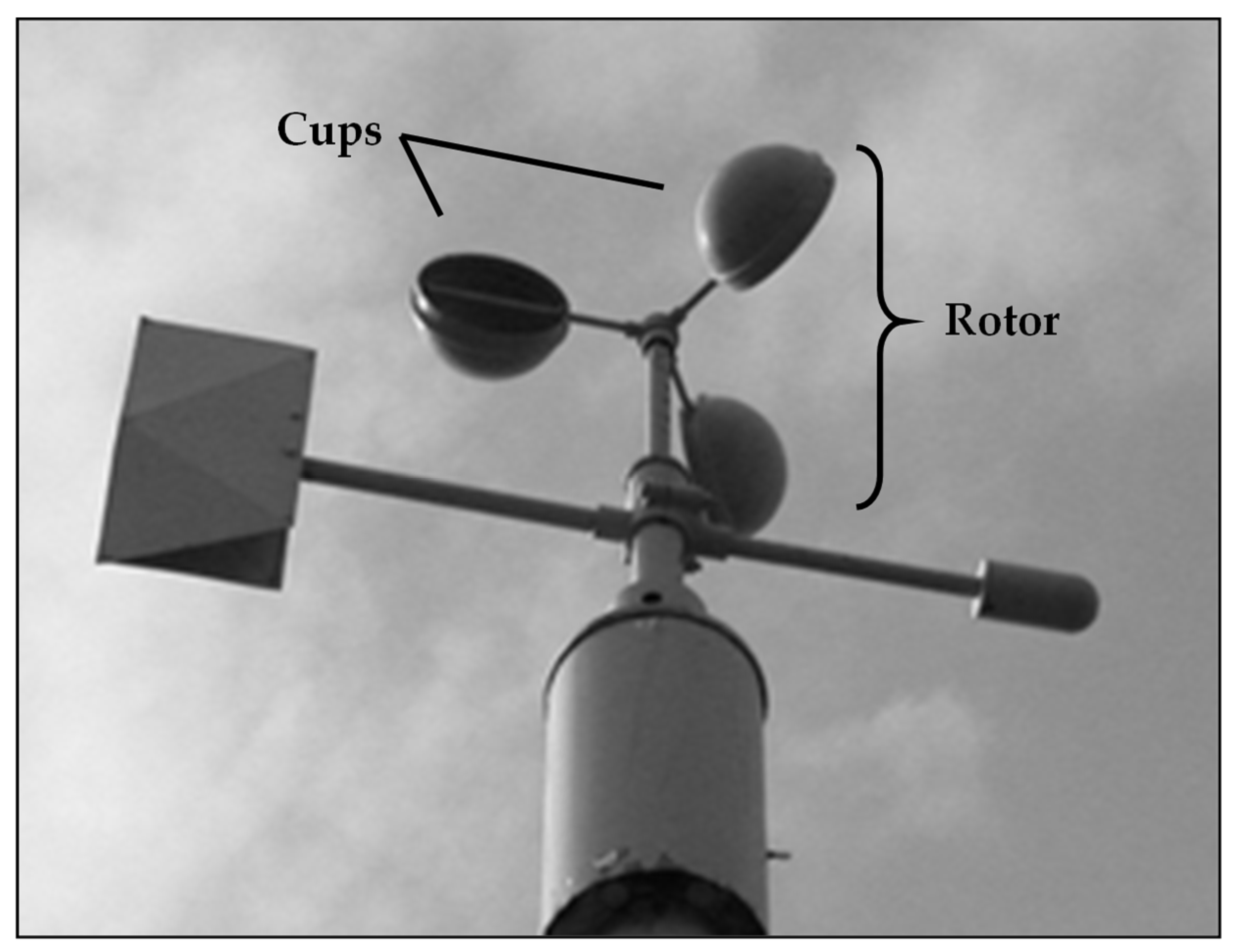
  • The ratio Rc/Rrc, between the radius of the cups, Rc, and the radius of rotation of the center of the cup, Rrc;
  • The cup’s normal force coefficient, cN, [12].
There are different models to relate the aerodynamic moment, QA, to the variables mentioned above [13,14,15]; however, these models have some limitations, such as that the cups’ normal force coefficients, cN, are provided based on measurements performed on static cups [16] (that is, they are not rotating), and precisely because the cups of an anemometer are rotating means that the point of application of the aerodynamic force on them is not the same as in a static situation. However, for the study of the problem at hand, it is reasonable to assume a linear relationship between the air density, ρ, and QA.
On the other hand, the friction torque, Qf, depends on the temperature, T, and the rotational speed of the anemometer rotor, ω, by means of the following expression:
Q f = B 0 + B 1 ω + B 2 ω 2 ,
where B0, B1, and B2 are coefficients that depend on the temperature, T [17].
The effect of temperature on cup anemometers has been studied with interest by several researchers. However, emphasis has almost always been placed on the effect of friction [11,18,19] and on the accumulation of ice on the cups when this instrument operates in extremely cold conditions [20,21,22,23,24,25,26].
The effect of air density variation on cup anemometer performance has received less attention from the scientific community, probably because this is a second-order effect when this instrument is used at altitudes not far from the one where it was calibrated. Changes in air density taken into account independently from air temperature seem to be possible only in extreme weather conditions or specific geographic locations.
This change in air density is an effect that alters the accuracy of an anemometer’s calibration curve (which relates the frequency of its output signal, f, or the frequency of rotor rotation, fr, to the incident air velocity over the instrument, V):
V = A f + B .
In the above equation, which is the transfer function of the anemometer, the coefficients A and B are called the calibration coefficients of the instrument.
Based on the authors’ search of the available literature, three scientific papers dealing with this problem can be highlighted. The first is the article by Schubauer and Mason in 1937 [27], the second is the technical report by Deutsche WindGuard GmbH (Varel, Germany) in 2018 [28], and the third is the publication of these latest results in 2023 [29].
This paper analyzes the effect of changes in air density on the performance of a cup anemometer (i.e., on the measured wind speed). This change in air density is produced by the location of the instrument, often in places with a high altitude in relation to the place where it has been calibrated and where the air density is significantly lower (e.g., air density values around ρ = 0.35 kg·m−3 have been observed in the Tibetan Plateau [30]). In addition, the possibility of using the cup anemometer in rare environments should not be overlooked. Examples include the cup anemometer designed to be carried on a probe designed at NASA’s Jet Propulsion Laboratory and intended to land on Mars [31], and the cup anemometer carried on the Venera 9 mission (1975) launched in 1975 for the planet Venus [32]. Furthermore, it should also be mentioned that quite recently, a cup anemometer was included in a stratospheric balloon mission (TASEC-Lab) as a wind speed sensor [33].
The work conducted in the above-mentioned publications is reviewed in Section 2 of this paper, where the data extracted from two of them [28,29] are analyzed. With this information, the impact of density variations on three different wind turbines’ Annual Energy Production (AEP) due to wind speed measurement errors is analyzed in Section 3. Finally, the conclusions of this work are included in Section 4.

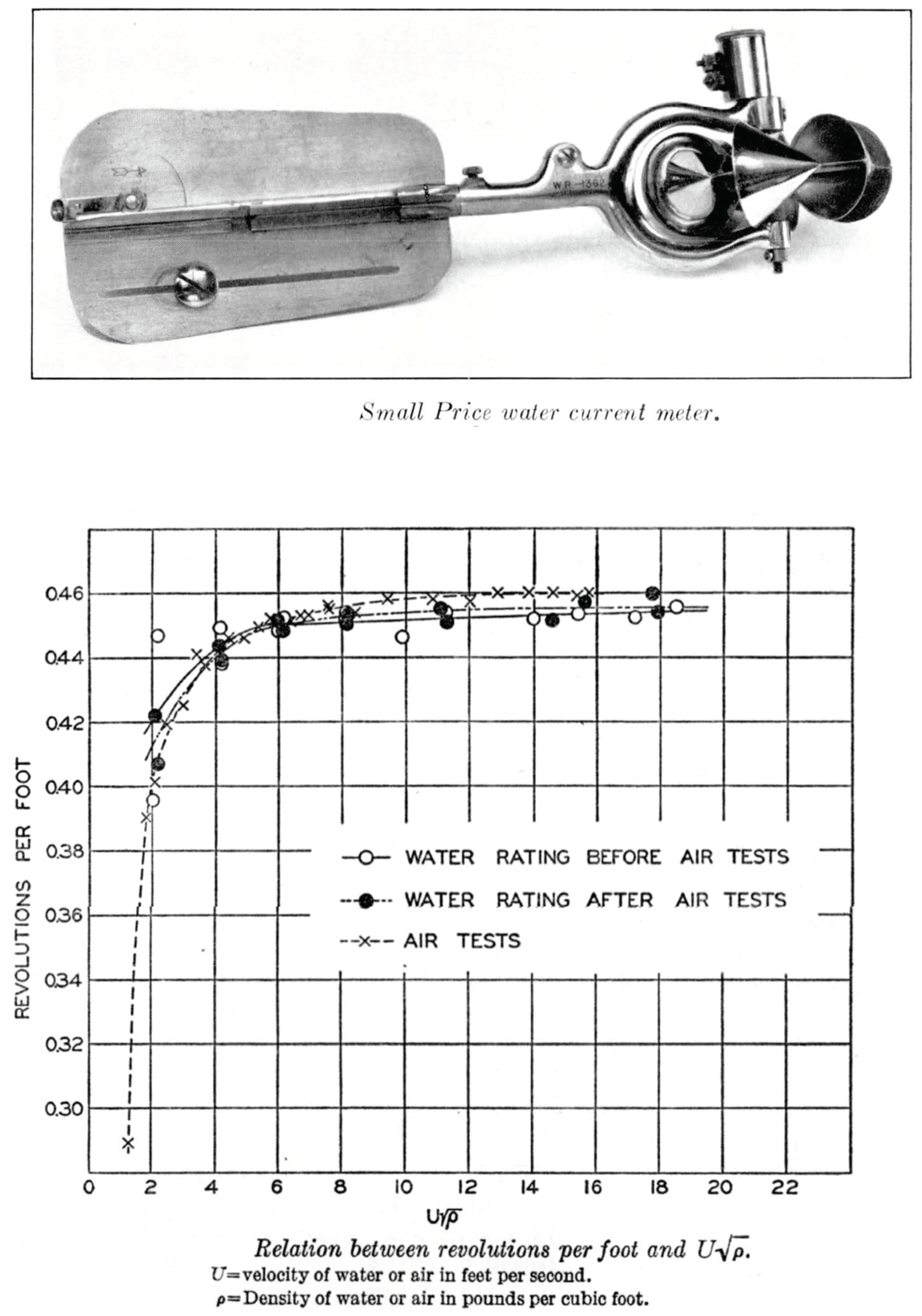
2. Effect of Air Density Variations on Cup Anemometers Performance—Research Carried Out in 1937 and 2018

The research by Schubauer and Mason [27] is particularly interesting and, unfortunately, appears to have been ignored by the scientific community since it does not appear in the Web of Science database and has only 10 citations in Google Scholar at the time of writing the present paper. These two authors studied the performance of a flow meter for fluids of different densities, air, and water whose morphology resembles that of a cup anemometer (see Figure 2).
In the work of these authors, it is shown that there is a fundamental parameter in the dynamics of the instrument, which is the relationship between friction and pressure forces. However, the effect of lowering the fluid density is greater than the effect of increasing it. Therefore, at low air densities, the cup anemometer should change its performance in relation to the one expected due to a different ratio between the aerodynamic and the friction forces (that is, the general assumption of neglecting the friction term in Equation (1) is no longer valid). Schubauer and Mason proposed the root of the dynamic pressure as the fundamental variable to represent the performances of the studied instrument:
V ρ = V 0 ρ 0 .
Thus, Figure 2 represents graphically the number of revolutions per unit of distance traveled by the wind. The points represented in the graph of this figure represent the one-to-one relationship between the rotation frequency, fr, and the wind speed, V, represented by the calibration curve of the instrument, i.e., Equation (3).
If we take the average results measured in the wind tunnel of a high precision cup anemometer such as the Thies Clima 4.3350: A = 0.0483 m y B = 0.248 m·s−1, and taking into account the annual average air density at the LAC-IDR/UPM laboratory where these calibrations were performed, ρ = 1.096 kg·m−3, and the number of pulses per revolution of that anemometer, Np = 37, it is possible to represent the calibration curve in the same terms as those used in the graph in Figure 2. Figure 3 shows a comparison between the calibration curve represented by the constants indicated above and the results of the air flow meter tests obtained by Schubauer and Mason. The comparison has been made with the data of revolutions per foot dimensioned with the number of turns per foot for 0.5 = 12 (expressed in United States customary units). This graph shows the great similarity between the two curves.
Once it has been established that the calibration curve is essentially composed of the points graphed by Schubauer and Mason (Figure 2) [27], it is possible to transfer the points of the graph of this figure to some graphs of what is today a cup anemometer calibration curve. Figure 4 shows these calibration curves (fluid velocity in m·s−1 represented in relation to the frequency of rotation of the instrument, fr, measured in both air and water). In both graphs, the equations of the linear regression fitted to the data have been included.
It is quite striking that the slopes of both curves are so similar. This means that the rotational speed of this instrument’s rotor at high speeds will be practically the same regardless of whether the fluid is air or water, whose density is much higher. However, it can be seen in the graph that, at low fluid velocities, the response of the instrument changes, becoming much lower in the case of the lower-density fluid; see Figure 5 for the percentage difference between the rotational frequencies in air, fr,a, and water, fr,w, at the same fluid speed, V, in relation to the rotational frequency in air, fr,a. This is mentioned in the work of Schubauer and Mason. Furthermore, these authors warn that this effect will be more relevant the lower the density of the fluids being compared.
As described in the first section of this article, thanks to the work of Deutsche WindGuard GmbH in 2018 [28], and later published in 2023 [29], information is available on the performance of a cup anemometer operating with air of different densities at a constant temperature.
Table 1 shows the plot data relating the performances of a cup anemometer as a function of air density [28,29]. The performances are analyzed with the variable k, defined as the rotational frequency divided by the fluid velocity divided by the same ratio measured for an air temperature T* = 20 °C and an atmospheric pressure P* = 1000 hPa:
k = f / V T ; P f / V T * ; P * .
These data were graphically extracted from the corresponding figure in the Deutsche WindGuard GmbH report [28]; see also Figure 6.
If the data in Table 1 are assumed to correspond to a Thies Clima 4.3350 cup anemometer (this detail is not clear from references [28,29], and could not be corroborated by the staff of Deutsche WindGuard GmbH. However, the reasoning stated hereafter can be applied to other First Class cup anemometer models such as any one of the Vector Instruments A100 series); the above-mentioned average calibration data of this instrument can be taken and, bearing in mind that these data were obtained with an air density ρ ~ 1.1 kg·m−3 (corresponding to average meteorological conditions in the city of Madrid (Spain)), it is possible to estimate the output frequencies of the instrument corresponding to the mentioned Table 1, see Table 2.
From here, it is possible to estimate the variation of the calibration constants A and B with the variation of the density. These variations have been plotted in the graph in Figure 7 for the density values studied. It can be observed in this graph that the values of both constants have been fitted to a fourth-order polynomial curve. Based on these fits, the value of both constants can be extrapolated to study the variation of the velocity measured by the cup anemometer as a function of the measured output frequency.
Figure 8 shows, as a function of the anemometer output frequency, f, the relationship between the wind speed that should be measured with respect to that measured with the calibration performed with a density ρ = 1.1 kg·m−3, V/Vρ=1.1, for three lower air densities (ρ = 0.95 kg·m−3, ρ = 0.8 kg·m−3 y ρ = 0.7 kg·m−3). It can be observed that for high frequencies the behavior is different than for low frequencies. For high frequencies, a decrease in density causes a decrease in the measured velocity, while for low frequencies, this tendency is reversed. We have chosen not to extrapolate the results using the settings shown in Figure 8 since for densities less than ρ = 0.7 kg·m−3, a greater decrease would imply zero or even negative values of the calibration constant B (Equation (3)). The constant B can never have a value B = 0 since there are always going to be wind speeds for which the anemometer starts or stops (these being different). This suggests a change in the trend shown by the constant B in Figure 7 for density values lower than ρ = 0.7 kg·m−3. Given the coupled behavior of both constants A and B (upon a change, e.g., in temperature or instrument wear, an increase in one of them usually corresponds to a decrease in the other), another change in trend can also be assumed for the other calibration constant, A. Therefore, it can be concluded that there is a large uncertainty in terms of the calibration of an anemometer for air velocity measurements at very low-density conditions.
Since the aerodynamic torque, QA, depends linearly on the dynamic pressure, it is reasonable to assume that the relationship between this variable and the torque produced by the friction forces, Qf, will be a determining parameter in the performances of the anemometer at least when faced with small variations in this relationship [11]. If the temperature of the cup anemometer bearings is constant, it can be assumed that the friction torque is constant, although as expressed in Equation (2), this frictional torque also depends (to a lesser extent [11]) on the rotational speed. Thus, in the absence of targeted experimental studies, a preliminary hypothesis suggests that, for very low air densities, the dynamic pressure (or the velocity times the root of the air density) should be considered a critical parameter. Variations in this parameter lead to variations in the cup anemometer’s performance.
This assumption (Equation (4)) has previously been made in studies concerning the use of this type of instrument in high-altitude conditions, such as stratospheric balloon missions [34]. However, it must be admitted that the results obtained in that research, although reasonable, should be re-evaluated with a new, more accurate model based on experimental results of the influence of air density variation on the performances of the cup anemometer.

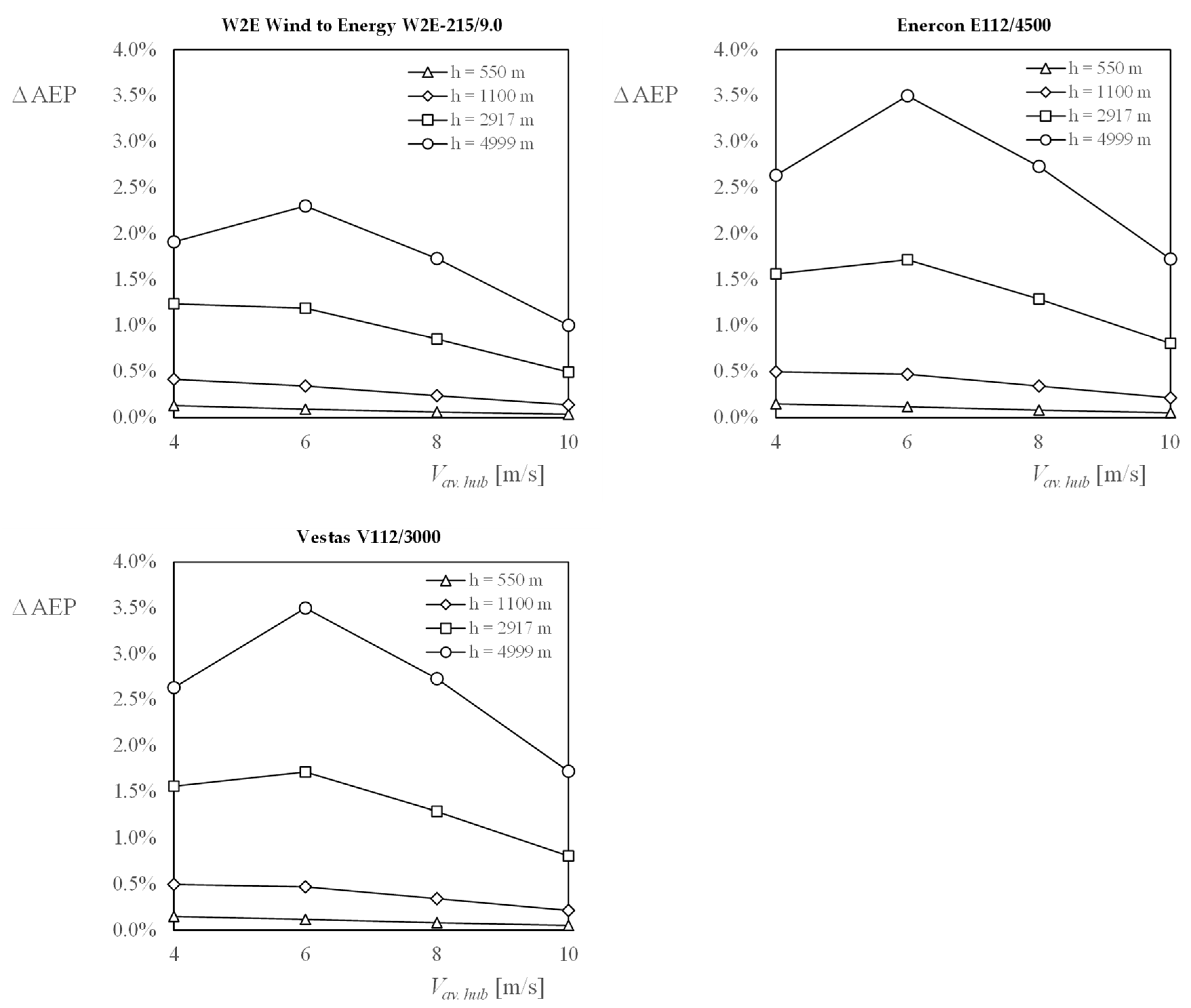
3. Estimation of Wind Turbine Annual Energy Production (AEP) Variations Caused by Errors in the Measured Wind Speed Due to Changes in the Air Density

In the previous section of this paper, the effect of air density variations on the performance of the cup anemometer was analyzed. It has been highlighted that use in conditions of air density different from those of the calibration of the instrument has an effect on the accuracy of its measurements, this effect being higher in conditions of less air density, that is, an anemometer calibrated at sea level but operating at 3000 m altitude introduces an error in the measurements that can be relevant.
The relevance of this error may not be striking at first glance. However, if one considers the effects at the level of wasted energy due to the lack of accuracy in imposing the best propeller pitch on a wind turbine, the error may be of sufficient importance to influence the decision to invest in a wind farm project or cause concerns regarding cost recovery.
Finally, the data in Figure 7, i.e., the calibration constants of the anemometer chosen for the calculations of this work (Thies Clima 4.3350) as a function of air density and the corresponding altitude above sea level, h, calculated assuming standard atmosphere [35]:
h = 44248 1 ρ 1.225 1 4.25 ,
have been included in Table 3.
With the coefficients included in Table 3, the variation of the Annual Energy Production (AEP) due to an error in the measured wind speed can be estimated (see Appendix A) for different wind turbines (i.e., different power curves associated with wind turbines) and different annual average speeds at hub height, Vav.hub [19,36]. It should be noted that in the present AEP estimations, only changes in the measured wind speed are considered, leaving aside the effect of the aerodynamics of the turbines’ blades.
For these calculations, the following wind turbines have been selected:
  • W2E Wind to Energy W2E-215/9.0 (Rostock, Germany). Rated Power 9000 kW.
  • Enercon E112/4500 (Aurich, Germany). Rated Power 4500 kW.
  • Vestas V112/3000 (Aarhus, Denmark). Rated Power 3000 kW.
Figure 9 shows the power curves of these wind turbines. The results in terms of the deviation of the Annual Energy Production (AEP) with respect to the ones obtained at sea level (h = 0 m) are shown in Figure 10 and Figure 11. As can be observed in the graphs from Figure 10, the deviation with respect to the AEP at sea level (h = 0 m) increases with the altitude at which the generators are installed. Moreover, the maximum deviation from the AEP occurs for speeds around 6 m/s, and this deviation affects less the higher power wind turbines (9000 kW) than lower power turbines (4500 kW and 3000 kW). The largest deviations obtained are around 3.5% for 4500 kW and 3000 kW wind turbines at speeds of 6 m·s−1. It is also fair to mention that air density changes also affect the power curves of the wind turbines. Therefore, the altitude at which a wind farm is planned to be installed can have a quite relevant effect on energy production as the power depends linearly on the air density [37,38]. The scope of the present work is limited to the effect of air density changes on wind speed measurements and its impact on the wind turbines AEP, but without considering the mentioned effect on the power curves.

4. Conclusions

In the present paper, the uncoupled effects of changes in the air density and temperature on cup anemometer performance are analyzed. The most relevant outlines are as follows:
  • The effect of air density changes on the cup anemometer measurements (this effect being uncoupled with the cup anemometer’s temperature, which affects the friction torque on the rotor’s shaft) has been studied by analyzing data available from open sources. The results indicate a change in the performance of the cup anemometer at air densities of around 0.65 kg·m−3. This change can be attributed to the ratio between aerodynamic and friction forces, as when the last ones are of the same order as the first ones; the classic aerodynamic theory that is applied to this instrument (the average dynamic torque is zero in one turn of the anemometer’s rotor), is no longer valid.
  • Additionally, the effect of the wind speed measurement bias on the Annual Energy Production of three wind generators due to air density variation with respect to the one from the instrument calibration has been estimated. The maximum impact is reached at wind speeds around 6 m·s−1, the consequences being a 1.5% AEP decrease at air densities corresponding to 2917 m above sea level. For higher altitudes, the effect is much more severe (3.5% decrease at around 5000 m above sea level). Larger wind generators (9000 kW instead of 3000–4500 kW) are less affected by the discrepancy between measured and true wind speed due to the difference in the air density between where the anemometer is operated and where it was calibrated.
  • More research is required to properly model the cup anemometer performance at air densities below 0.7 kg·m−3. This could help to extend the use of the cup anemometer to stratospheric balloons, bearing in mind the errors of sonic anemometers in these conditions due to the problems related to the sonic transmittance in low-density air.

Author Contributions

Conceptualization, S.P., D.A.-C., I.T.-G. and F.M.-G.; methodology, S.P. and D.A.-C.; validation, S.P. and D.A.-C.; formal analysis, S.P. and D.A.-C.; investigation, S.P. and D.A.-C.; data curation, S.P., D.A.-C., I.T.-G. and F.M.-G.; writing—original draft preparation, S.P., D.A.-C., I.T.-G. and F.M.-G.; writing—review and editing, S.P., D.A.-C., I.T.-G. and F.M.-G.; supervision, S.P. All authors have read and agreed to the published version of the manuscript.

Funding

This research received no external funding.

Data Availability Statement

The raw data supporting the conclusions of this article will be made available by the authors on request.

Acknowledgments

The authors gratefully acknowledge Ángel Sanz-Andrés for his encouraging support regarding the research program on cup anemometer performance. The authors are indebted to the reviewers, whose comments helped to improve the present paper.

Conflicts of Interest

The authors declare no conflict of interest.

Appendix A

The estimation of the AEP variations caused by deviations of the wind speed data provided by the cup anemometer has been obtained following the EN IEC 61400-12-1:2022 standard [19], which provides the procedure for estimating the AEP of wind turbines. The procedure states that the AEP is obtained with the following equation:
AEP = N h i = 1 N F V i F V i 1 P i 1 + P i 2 ,
where Nh is the number of hours in a year, N is the number of analyzed wind speeds, Vi is the normalized and averaged wind speed of the wind turbine power curve, F(Vi) is the Rayleigh cumulative probability distribution function for wind speed Vi, and Pi is the normalized and averaged power output for the wind turbine at wind speed Vi. The Rayleigh cumulative probability distribution is defined as follows:
F ( V ) = 1 exp π 4 V V a v e 2 ,
where V is the evaluated wind speed, and Vave is the annual measured average wind speed.
Taking the above into account, the deviations caused by differences in air density are introduced as deviations in the annual measured average wind speed, which changes the Rayleigh probability distribution, thus modifying the estimated AEP for the given power curves. The influence of air density in the wind turbine power curves is not analyzed in this work. However, air density may also affect the wind turbine power curves and, consequently, the AEP estimations. The AEP estimations included in the present research were carried out with a simple spreadsheet.

References

  1. Robinson, T.R. II. On the Determination of the Constants of the Cup Anemometer by Experiments with a Whirling Machine. Proc. R Soc. Lond. 1878, 27, 286–289. [Google Scholar] [CrossRef]
  2. Robinson, T.R. XXIII. On the Determination of the Constants of the Cup Anemometer by Experiments with a Whirling Machine. Philos. Trans. R Soc. Lond. 1878, 169, 777–822. [Google Scholar] [CrossRef]
  3. Robinson, T.R. On the Constants of the Cup Anemometer. Proc. R. Soc. Lond. 1880, 30, 572–574. [Google Scholar]
  4. Pedersen, T.F.; Dahlberg, J.-Å. Modelling of cup anemometry and dynamic overspeeding in average wind speed measurements. Egusph 2023. preprint. [Google Scholar] [CrossRef]
  5. Sanz-Andrés, A.; Pindado, S.; Sorribes, F. Mathematical analysis of the effect of the rotor geometry on cup anemometer response. Sci. World J. 2014, 2014, 537813. [Google Scholar] [CrossRef]
  6. Li, R.; Kikumoto, H. Journal of Wind Engineering & Industrial Aerodynamics Data-driven calibration of cup anemometer based on field measurements and artificial neural network for wind measurement around buildings. J. Wind Eng. Ind. Aerodyn. 2022, 231, 105239. [Google Scholar] [CrossRef]
  7. Dai, S.; Sweetman, B. Physics-based recalibration method of cup anemometers. Flow Meas. Instrum. 2023, 91, 102343. [Google Scholar] [CrossRef]
  8. Azorin-molina, C.; Pirooz, A.A.S.; Bedoya-Valestt, S.; Utrabo-Carazo, E.; Andres-Martin, M.; Shen, C.; Minola, L.; Guijarro, J.A.; Aguilar, E.; Brunet, M.; et al. Biases in wind speed measurements due to anemometer changes. Atmos. Res. 2023, 289, 106771. [Google Scholar] [CrossRef]
  9. Ligęza, P. Dynamic Error Correction Method in Tachometric. Energies 2022, 15, 4132. [Google Scholar] [CrossRef]
  10. Wolken-m, G.; Bischoff, O.; Gottschall, J. Analysis of wind speed deviations between floating lidars, fixed lidar and cup anemometry based on experimental data Analysis of wind speed deviations between floating lidars, fixed lidar and cup anemometry based on experimental data. J. Phys. Conf. Ser. 2022, 2362, 012042. [Google Scholar] [CrossRef]
  11. Alfonso-Corcuera, D.; Pindado, S.; Ogueta-Guitiérrez, M.; Sanz-Andrés, Á. Bearing friction effect on cup anemometer performance modelling. J. Phys. Conf. Ser. 2021, 2090, 012101. [Google Scholar] [CrossRef]
  12. Roibas-Millan, E.; Cubas, J.; Pindado, S. Studies on cup anemometer performances carried out at IDR/UPM Institute. Past and present research. Energies 2017, 10, 1860. [Google Scholar] [CrossRef]
  13. Ramachandran, S. A theoretical study of cup and vane anemometers. Q. J. R. Meteorol. Soc. 1969, 95, 163–180. [Google Scholar] [CrossRef]
  14. Ramachandran, S. A theoretical study of cup and vane anemometers—Part II. Q. J. R. Meteorol. Soc. 1969, 96, 115–123. [Google Scholar] [CrossRef]
  15. Wyngaard, J.C. Cup, propeller, vane, and sonic anemometers in turbulence research. Annu. Rev. Fluid Mech. 1981, 13, 399–423. [Google Scholar] [CrossRef]
  16. Brevoort, M.J.; Joyner, U.T. Experimental Investigation of the Robinson-Type Cup Anemometer; No. NACA-TR-513; NASA Technical Reports Server: Washington, DC, USA, 1936. [Google Scholar]
  17. IEC 61400-50-1:2022; Wind Energy Generation Systems—Part 50-1: Wind Measurement—Application of Meteorological Mast, Nacelle and Spinner Mounted Instruments. International Electrotechnical Commission: Geneva, Switzerland, 2022.
  18. Fabian, O. Fly-Wheel Calibration of Cup-Anemometers. Risø-R-797(EN): Contributions from the Department of Meteorology and Wind Energy to the EWEC’94 Conference in Thessaloniki, Greece; Risø National Laboratory: Roskilde, Denmark, 1995. [Google Scholar]
  19. IEC 61400-12-1:2022; Wind Turbines. Part 12-1: Power Performance Measurements of Electricity Producing Wind Turbines. International Electrotechnical Commission: Geneva, Switzerland, 2005.
  20. Tammelin, B.; Cavaliere, M.; Kimura, S.; Morgan, C.; Peltomaa, A. Ice Free Anemometers. In Proceedings of the BOREAS IV, Proceeding of an International Meeting; Finnish Meteorological Institute: Helsinki, Finland, 1998; pp. 239–252. [Google Scholar]
  21. Kimura, S.; Abe, K.; Tsuboi, K.; Tammelin, B.; Suzuki, K. Aerodynamic characteristics of an iced cup-shaped body. Cold Reg. Sci. Technol. 2001, 33, 45–58. [Google Scholar] [CrossRef]
  22. Makkonen, L.; Lehtonen, P.; Helle, L. Anemometry in icing conditions. J. Atmos. Ocean. Technol. 2001, 18, 1457–1469. [Google Scholar] [CrossRef]
  23. Fortin, G.; Perron, J.; Ilinca, A. Behaviour and Modeling of Cup Anemometers under Icing Conditions. In Proceedings of the 11th International Workshop on Atmospheric Icing of Structures, Montréal, QC, Canada, 12–16 June 2005. [Google Scholar]
  24. Bégin-Drolet, A.; Ruel, J.; Lemay, J. Off-axis characterization of ice-free anemometers. J. Wind Eng. Ind. Aerodyn. 2011, 99, 825–832. [Google Scholar] [CrossRef]
  25. Bégin-Drolet, A.; Ruel, J.; Lemay, J.; Giroux, G. Commissioning of a new ice-free anemometer: 2011 Field tests at WEICan. Measurement 2012, 45, 2029–2040. [Google Scholar] [CrossRef]
  26. Bégin-Drolet, A.; Lemay, J.; Ruel, J. Time domain modeling of cup anemometers using artificial neural networks. Flow Meas. Instrum. 2013, 33, 10–27. [Google Scholar] [CrossRef]
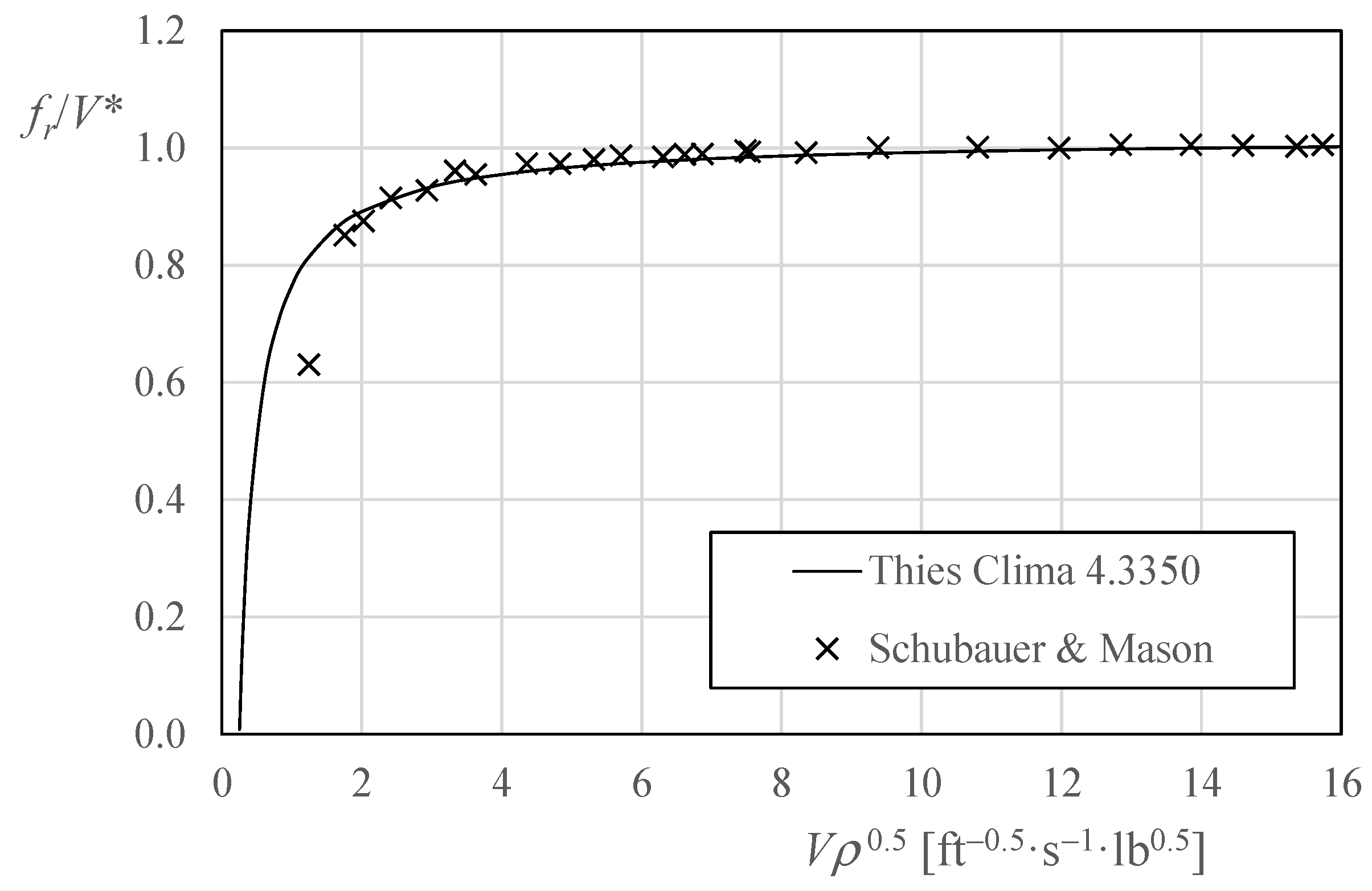
  27. Schubauer, G.B.; Mason, M.A. Performance characteristics of a water current meter in water and in air. J. Res. Natl. Bur. Stand. 1937, 18, 351–360. [Google Scholar] [CrossRef]
  28. Busche, P.; May, C.; Roß, A.; Suhr, J.; Westermann, H. Anemometer Calibration at Different Air Temperatures and Air Pressures. Project No.: VT180259. Report No.: VT180259_01_Rev0. Report Date: 2018-03-02.
  29. Roß, A.; Balaresque, N.; Fischer, A. Temperature and pressure effects on the response behavior of anemometers. Tech. Mess. 2023, 90, 604–612. [Google Scholar] [CrossRef]
  30. Liang, Y.; Ji, X.; Wu, C.; He, J.; Qin, Z. Estimation of the influences of air density on wind energy assessment: A case study from China. Energy Convers. Manag. 2020, 224, 113371. [Google Scholar] [CrossRef]
  31. Wellman, J.B. A Folding Rotating Cup Anemometer. In Space Programs Summary 37-53, Vol. III. Supporting Research and Advanced Development For the Period August 1 to September 30, 1968; NASA, Jet Propulsion Laboratory, California Institute of Technology: Pasadena, CA, USA, 1968; pp. 133–143. [Google Scholar]
  32. Lorenz, R.D. Surface winds on Venus: Probability distribution from in-situ measurements. Icarus 2016, 264, 311–315. [Google Scholar] [CrossRef]
  33. González-Bárcena, D.; Peinado-Pérez, L.; Fernández-Soler, A.; Pérez-Muñoz, Á.G.; Álvarez-Romero, J.M.; Ayape, F.; Martín, J.; Bermejo-Ballesteros, J.; Porras-Hermoso, Á.L.; Alfonso-Corcuera, D.; et al. TASEC-Lab: A COTS-based CubeSat-like university experiment for characterizing the convective heat transfer in stratospheric balloon missions. Acta Astronaut. 2022, 196, 244–258. [Google Scholar] [CrossRef]
  34. Alfonso-Corcuera, D.; Ogueta-Guitiérrez, M.; Fernández-Soler, A.; González-Bárcena, D.; Pindado, S. Measuring Relative Wind Speeds in Stratospheric Balloons with Cup Anemometers: The TASEC-Lab Mission. Sensors 2022, 22, 5575. [Google Scholar] [CrossRef]
  35. Pindado, S. Elementos de Transporte Aéreo; Meseguer, J., Sanz-Andrés, A., Eds.; Instituto Universitario de Microgravedad “Ignacio Da Riva”: Madrid, Spain, 2006; ISBN 84-921113-9-9. [Google Scholar]
  36. IEC 61400-12-1:2017; Wind Energy Generation Systems. Power Performance Measurements of Electricity Producing Wind Turbines. International Electrotechnical Commission: Geneva, Switzerland, 2017.
  37. Kusiak, A.; Zheng, H.; Song, Z. On-line monitoring of power curves. Renew. Energy 2009, 34, 1487–1493. [Google Scholar] [CrossRef]
  38. Carrillo, C.; Obando Montaño, A.F.; Cidrás, J.; Díaz-Dorado, E. Review of power curve modelling for windturbines. Renew. Sustain. Energy Rev. 2013, 21, 572–581. [Google Scholar] [CrossRef]
Figure 1. Cup anemometer installed over a wind vane. The cups and the rotor of this instrument are indicated in the figure. Photo courtesy of the Agencia Estatal de Meteorología (AEMET), Spain. http://hdl.handle.net/20.500.11765/11425, accessed on 22 December 2023.
Applsci 14 01843 g001
Figure 2. (Top) Current meter tested with water and air flow by Schubauer and Mason [27]. (Bottom) Some of the results of the testing campaign. Revolutions per foot, fr/V, in relation to the flow speed, V, multiplied by the square ratio of the flow density, ρ. Reprinted with permission from the National Institute of Standards and Technology, U.S. Department of Commerce. Not copyrightable in the United States.
Applsci 14 01843 g002
Figure 3. Non-dimensional rotation rate per length unit, fr/V*, of the Thies Clima 4.3350 cup anemometer and the flow meter tested by Schubauer and Mason [27], in relation to the product of wind speed and the square ratio of the air density, 0.5.
Applsci 14 01843 g003
Figure 4. Data points from the graph included in Figure 2 (Top: Air tests; Bottom: Water rating after air tests), expressed in terms of fluid velocity, V, in relation to the instrument’s rotation frequency, fr.
Applsci 14 01843 g004
Figure 5. Percentage difference between the rotational frequencies in air, fr,a, and water, fr,w, at the same fluid speed, V, in relation to the rotational frequency in air, fr,a.
Applsci 14 01843 g005
Figure 6. Variable k (Equation (5)) as a function of the air density, ρ, for different wind speeds. Data from wind tunnel testing extracted graphically from the Deutsche WindGuard GmbH report 2018 [28].
Applsci 14 01843 g006
Figure 7. Calibration constants A and B (Equation (3)) calculated with the data from Table 2.
Applsci 14 01843 g007
Figure 8. Wind speed measured with respect to that measured with the calibration performed with a density ρ = 1.1 kg·m−3, V/Vρ=1.1, in relation to the cup anemometer’s output frequency, f, for three lower air densities (ρ = 0.95 kg·m−3, ρ = 0.8 kg·m−3 and ρ = 0.7 kg·m−3).
Applsci 14 01843 g008
Figure 9. Power curves of W2E Wind to Energy W2E-215/9.0, Enercon E112/4500, and Vestas V112/3000 wind turbines.
Applsci 14 01843 g009
Figure 10. Percentage variation of the Annual Energy Production, ΔAEP, of wind turbines W2E Wind to Energy W2E-215/9.0 (Top-Left), Enercon E112/4500 (Top-Right) and Vestas V112/3000 (Bottom), due to the error of the measured wind speed caused by the air density change (related to the air density during the instrument calibration process), in relation to the height over the sea level, h, for annual average wind speeds at hub height Vav.hub = 4, 6, 8 and 10 m·s−1.
Applsci 14 01843 g010
Figure 11. Percentage variation of the Annual Energy Production, ΔAEP, of wind turbines W2E Wind to Energy W2E-215/9.0 (Top-Left), Enercon E112/4500 (Top-Right) and Vestas V112/3000 (Bottom), due to the error of the measured wind speed caused by the air density change (related to the air density during the instrument calibration process), in relation to the annual average wind speed at hub height, Vav.hub, for heights over the sea level h, =550, 1100, 2917 and 4999 m.
Applsci 14 01843 g011
Table 1. Variable k (Equation (5)) as a function of the wind speed, V, and the air density, ρ. Data from wind tunnel testing extracted graphically from the Deutsche WindGuard GmbH report 2018 [28].
ρ [kg·m−3]V [m·s−1]
15.5141210864
0.8550.980580.986430.989230.99090.992070.992860.99336
0.9160.986410.990090.991880.993050.993720.994220.99452
0.9760.989030.992240.993790.994790.99550.995960.99617
1.0380.991980.994360.995360.996070.996610.996740.99691
1.1000.996890.997480.997770.99810.998140.998310.99823
1.1610.999380.999420.999590.999550.999460.999510.99938
1.2271.000331.000171.000121.000211.000251.000211.00021
1.2941.003541.002281.001821.001611.001151.001161.00107
1.3521.003231.002521.002061.001681.001471.001391.00122
Table 2. Output frequencies corresponding to the data from Table 1, supposing that the cup anemometer used in this testing was a Thies Clima 4.3350 cup anemometer.
ρ [kg·m−3]V [m·s−1]
15.5141210864
0.855310.61281.57241.23200.45159.52118.4477.30
0.916312.46282.61241.88200.88159.79118.6077.39
0.976313.29283.23242.34201.23160.07118.8177.52
1.038314.22283.83242.73201.49160.25118.9077.58
1.100315.78284.72243.31201.90160.50119.0977.68
1.161316.57285.28243.76202.20160.71119.2377.77
1.227316.76285.44243.86202.29160.79119.2977.82
1.294317.88286.09244.30202.61160.98119.4377.90
1.352317.78286.16244.36202.63161.03119.4677.91
Table 3. Variation of the calibration constants of a Thies Clima 4.3350 anemometer (estimated mean values) with altitude above sea level, h. These coefficients are based on the data included in Table 2.
h [m]A [m]B [m·s−1]
00.04810.2579
5500.04820.2574
11000.04830.2480
16860.04860.2238
22950.04870.2083
29170.04890.2017
35860.04920.1696
49990.04990.0986
Disclaimer/Publisher’s Note: The statements, opinions and data contained in all publications are solely those of the individual author(s) and contributor(s) and not of MDPI and/or the editor(s). MDPI and/or the editor(s) disclaim responsibility for any injury to people or property resulting from any ideas, methods, instructions or products referred to in the content.

