


Pruning Quantized Unsupervised Meta-Learning DegradingNet Solution for Industrial Equipment and Semiconductor Process Anomaly Detection and Prediction


Abstract
1. Introduction
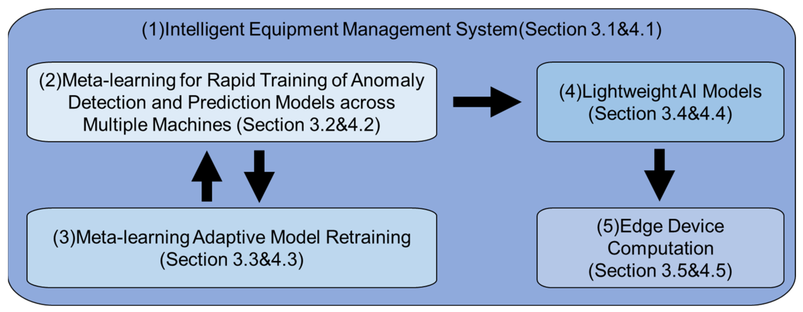
- (1)
- Intelligent Equipment Management System (Section 3.1 and Section 4.1)
- (2)
- Meta-learning for Rapid Training of Anomaly Detection and Prediction Models across Multiple Machines (Section 3.2 and Section 4.2)
- (3)
- Meta-learning Adaptive Model Retraining (Section 3.3 and Section 4.3)
- (4)
- Lightweight AI Models (Section 3.4 and Section 4.4)
- (5)
- Edge Device Computation (Section 3.5 and Section 4.5)
2. Related Study
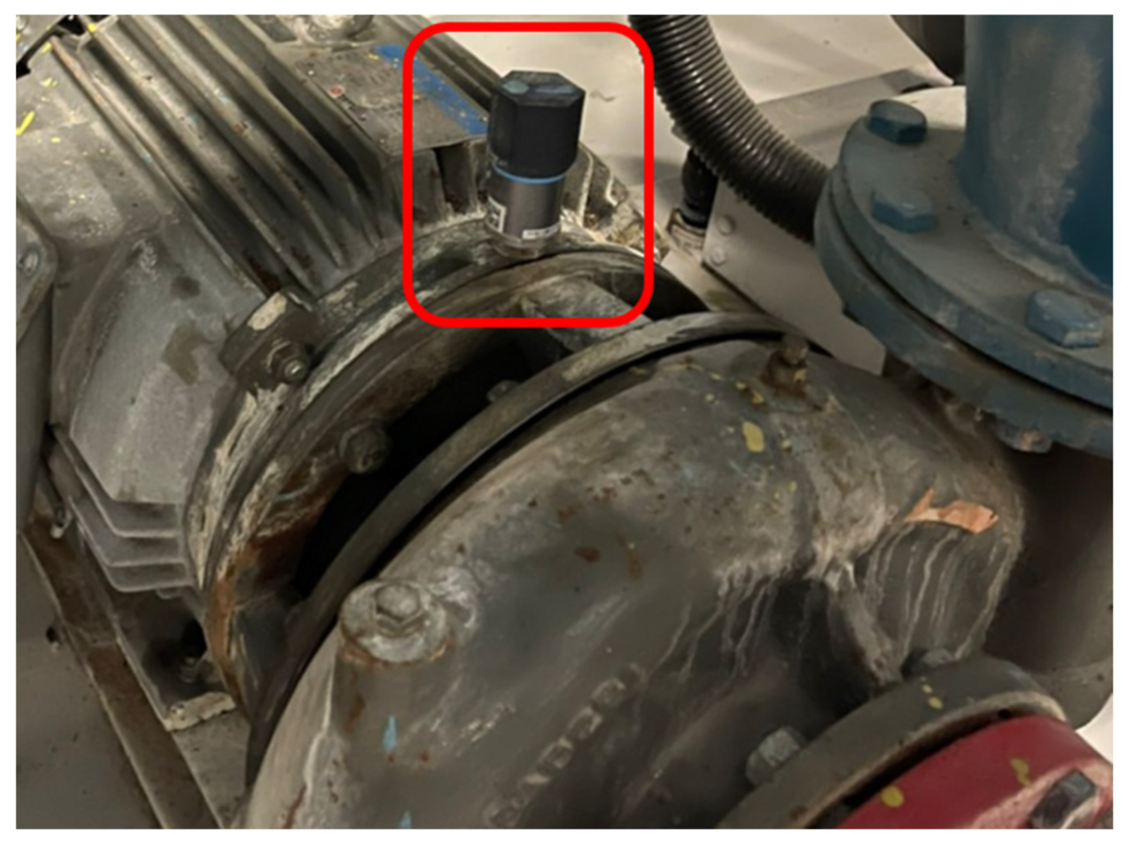
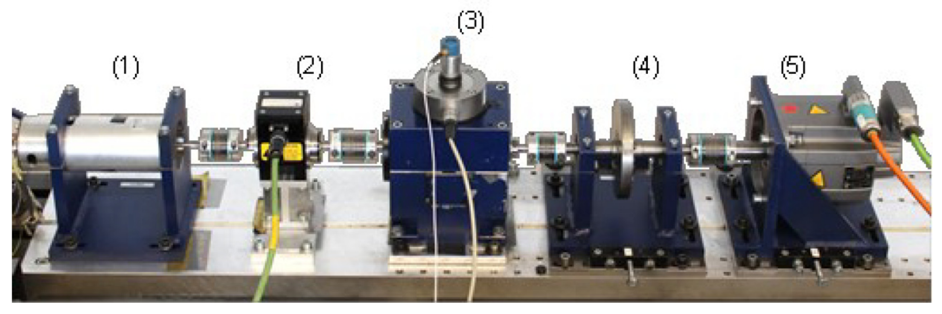
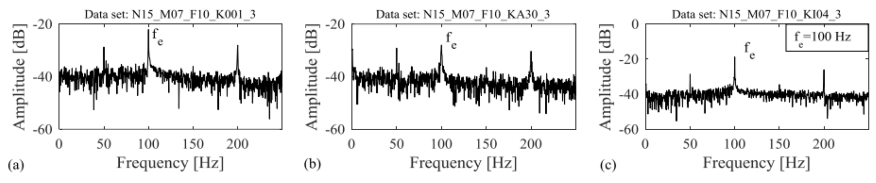
2.1. Vibration Signal Data Acquisition
- (1)
- Device Sensors
- (2)
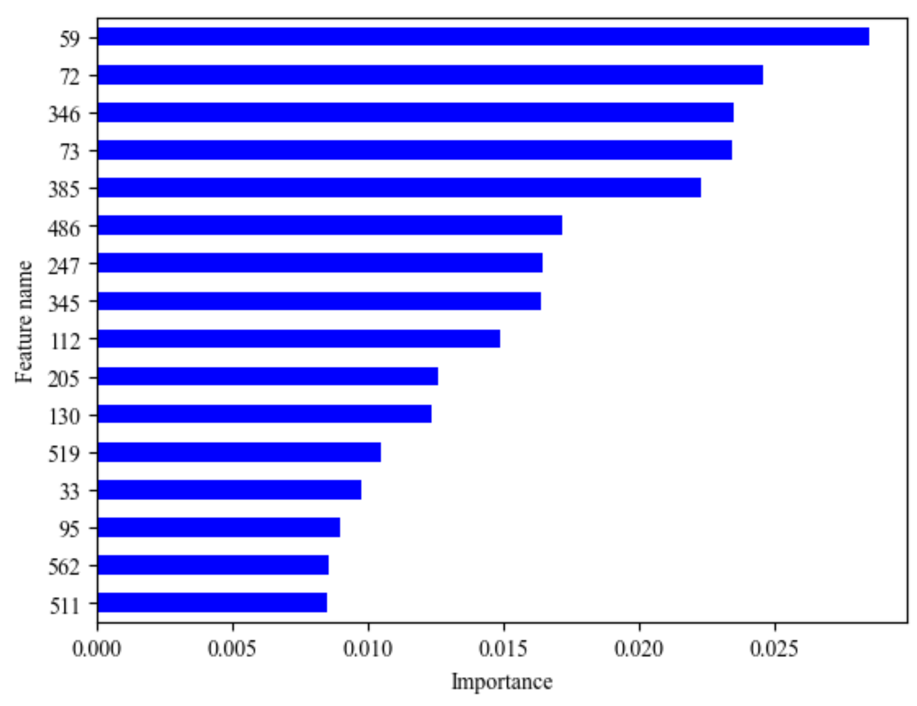
- Vibration Data Feature Transformation
2.2. Vibration Signal Data of Chiller
2.3. Paderborn University Bearing Dataset
2.4. SECOM Semiconductor Analysis Dataset
2.5. Data Preprocessing
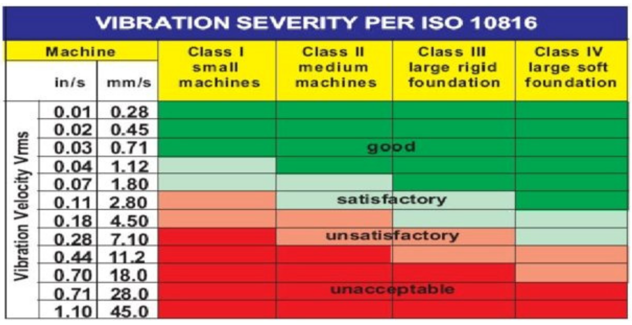
2.6. Equipment Process Degradation Level
2.7. Equipment Process Data Storage
2.8. Area under Curve
3. Proposed Method
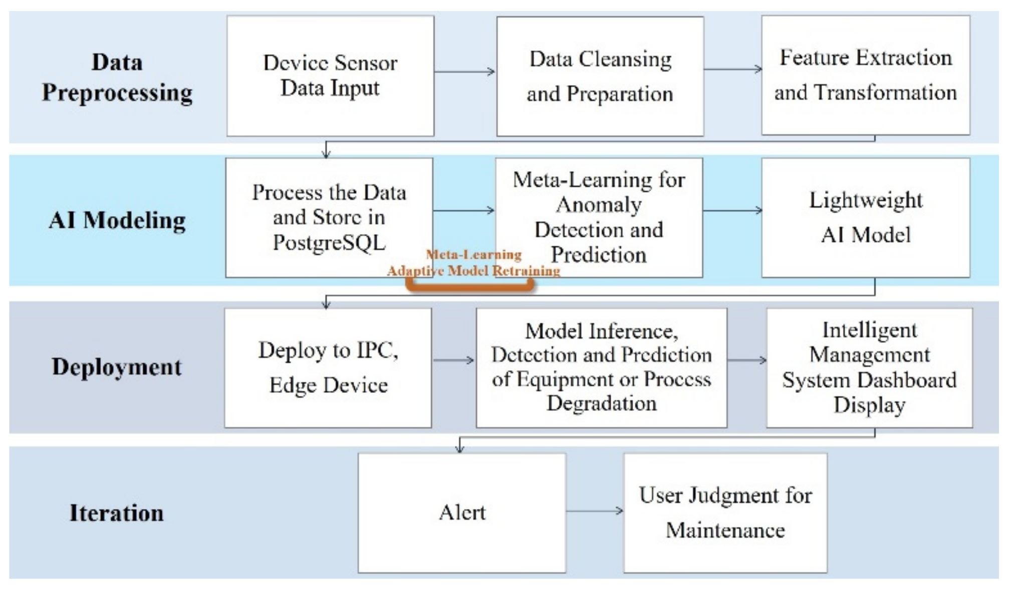
3.1. Intelligent Equipment Management System
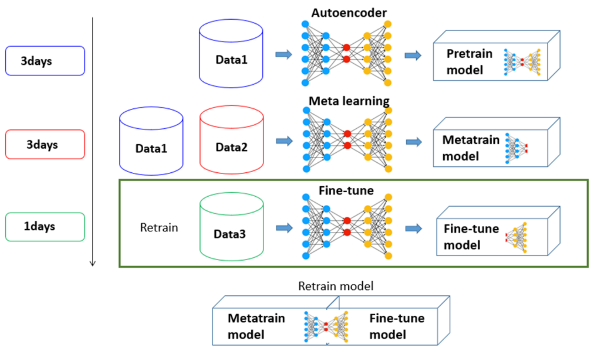
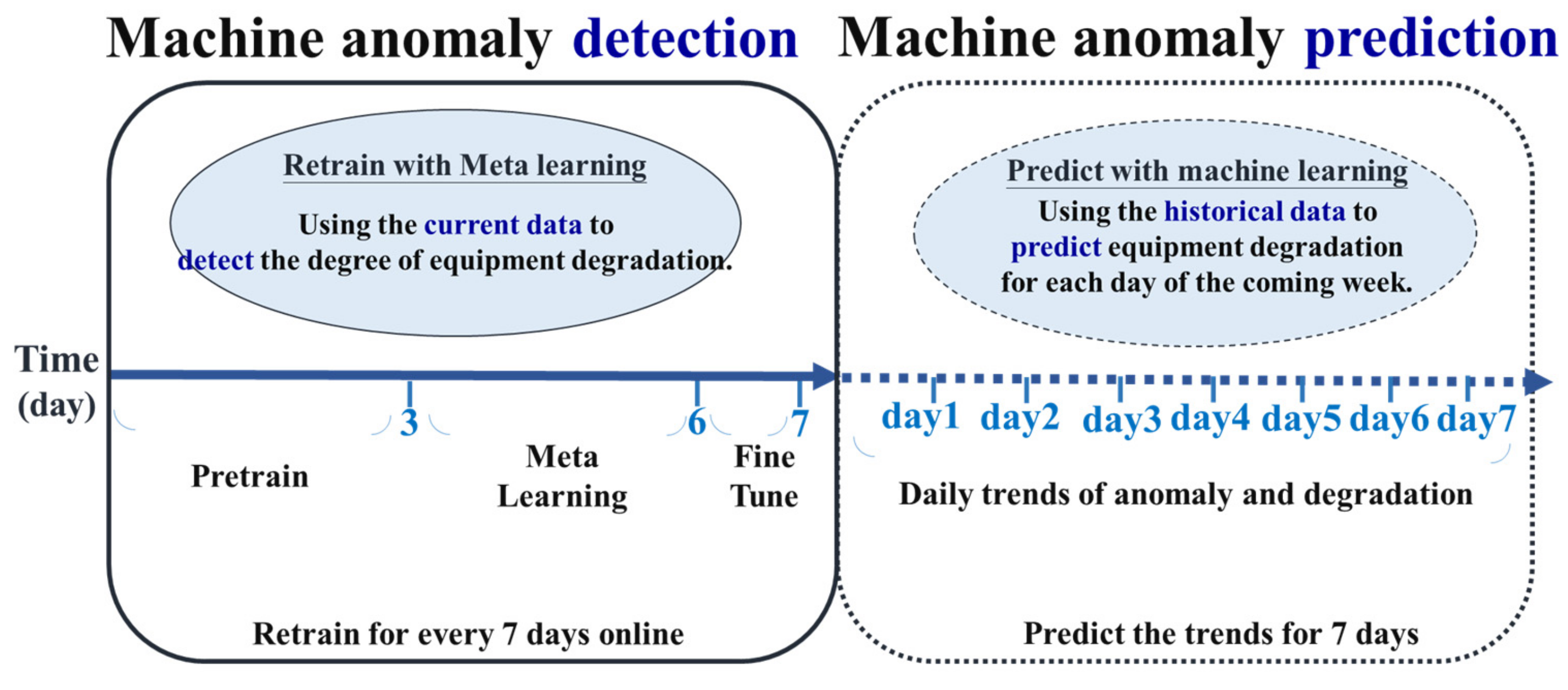
3.2. Meta-Learning for Rapid Training of Multi-Machine Models for Anomaly Detection and Prediction
- (1)
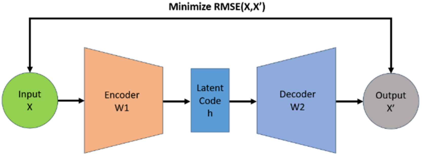
- Meta-learning
- (2)
- Anomaly Detection
- (3)
- Anomaly Prediction
- (a)
- Simple Exponential Smoothing (SES)
- (b)
- Holt (Double Exponential Smoothing Method)
- (c)
- Holt–Winters Forecasting (Triple Exponential Smoothing)
- (d)
- Autoregressive Model
- (e)
- Moving Average
- (f)
- Autoregressive Integrated Moving Average
- (g)
- Seasonal Autoregressive Integrated Moving Average
3.3. Meta-Learning Adaptive Model Retraining
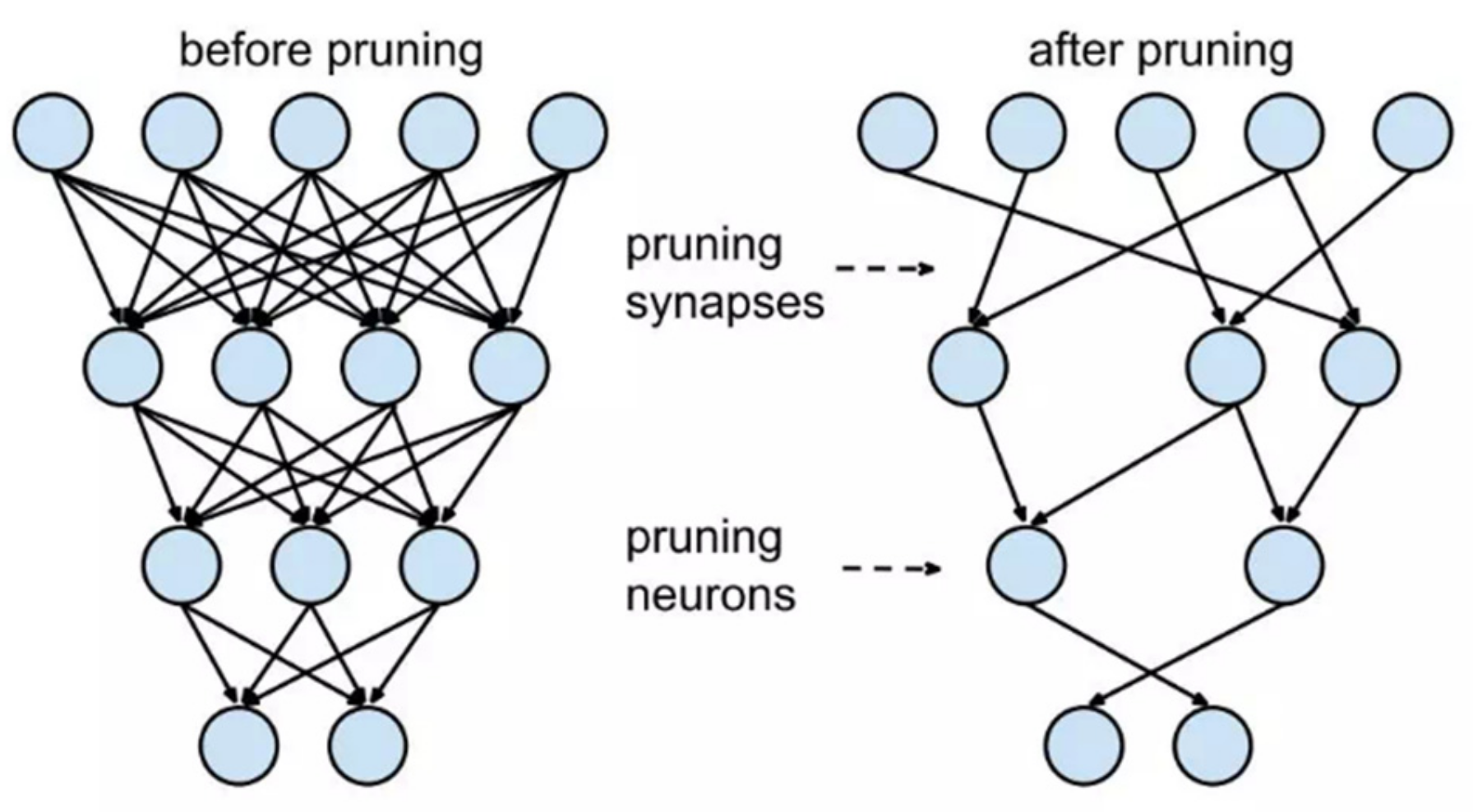
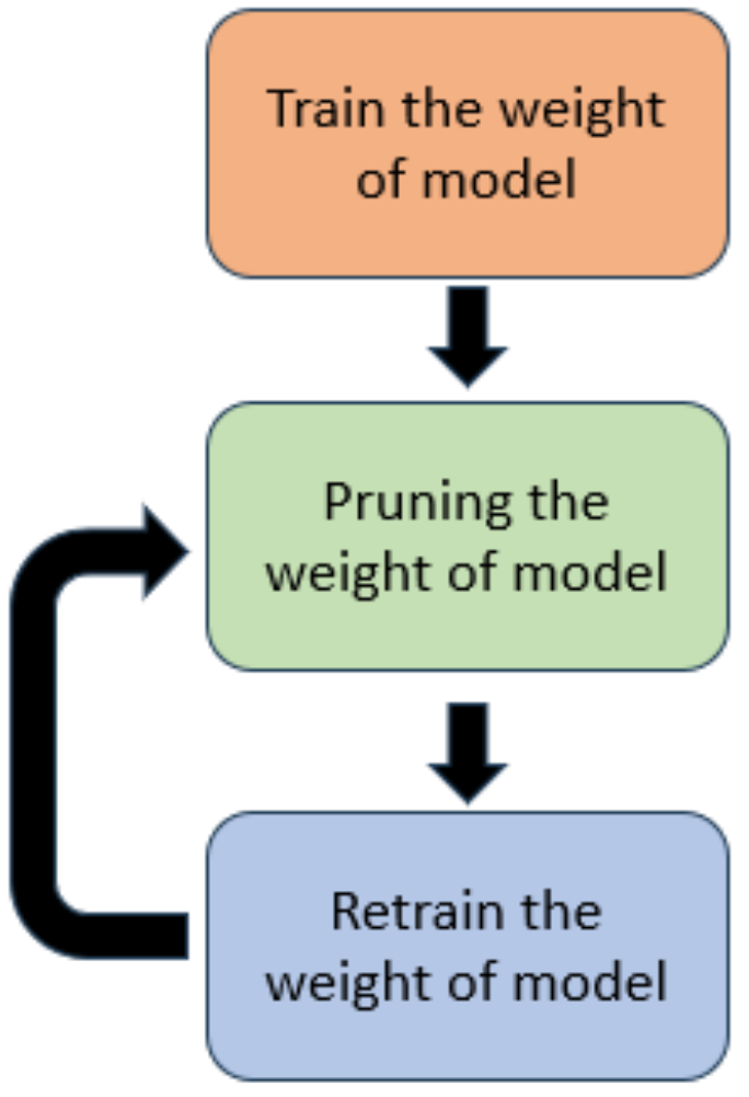
3.4. Lightweight AI Model
- (1)
- Model Pruning
- (2)
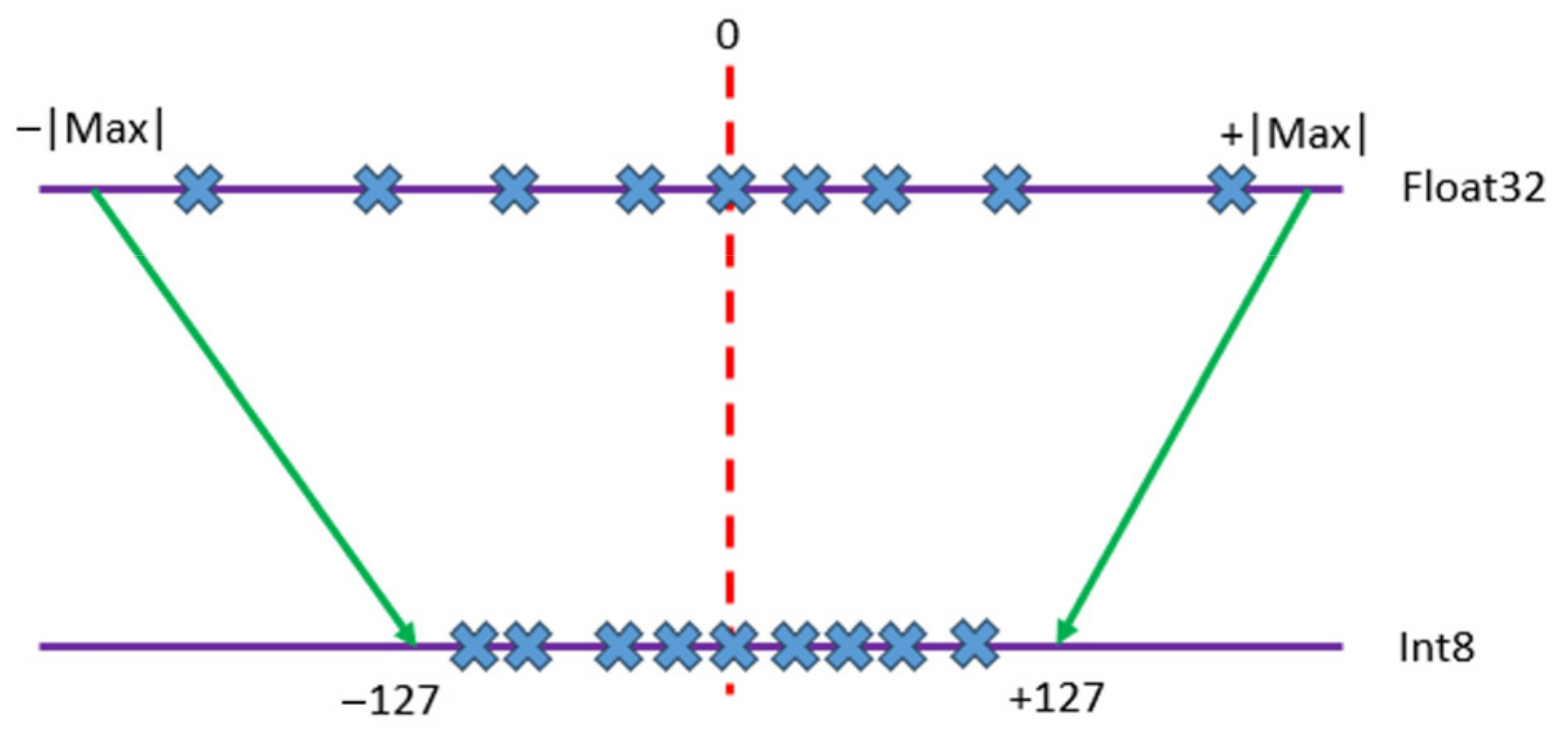
- Model Quantization
3.5. Edge Device Computing
- Provides rapid real-time reflection of situations, enabling onsite personnel to detect anomalies promptly and take immediate action.
- Solves bandwidth issues in cloud and edge transmissions because edge devices only need to send inference results back to the control centers.
- Addresses cybersecurity concerns, protecting against network attacks that could lead to factory shutdowns.
- Reduces energy consumption because lightweight edge-computing models conserve power.
4. Results and Discussion
4.1. Intelligent Equipment Management System
4.2. Meta-Learning for Rapid Training of Multi-Machine Models for Anomaly Detection and Prediction
- (1)
- Rapid Training of Multi-Machine Models for Anomaly Detection
- (2)
- Anomaly Prediction:
4.3. Meta-Learning Adaptive Model Retraining
4.4. Lightweight AI Model
4.5. Edge Device Computing
5. Conclusions
Author Contributions
Funding
Data Availability Statement
Acknowledgments
Conflicts of Interest
Nomenclature
| AE | Autoencoder |
| AI | Artificial Intelligence |
| AR | Autoregressive |
| ARIMA | Autoregressive Integrated Moving Average |
| AUC | Area under Curve |
| DAE | Deep AE |
| FFT | Fast Fourier Transform |
| IPC | Industrial Personal Computer |
| LoRaWAN | Long-Range Wide-Area Network |
| MA | Moving Average |
| MCM | Machine Condition Monitoring |
| MCS | Motor Current Signal |
| ML | Machine Learning |
| PHM | Prognostics and Health Management |
| PQUM-DNS | Pruning Quantized Unsupervised Meta-learning DegradingNet Solution |
| PSD | Power Spectral Density |
| RMS | Root Mean Square |
| RMSE | Root Mean Square Error |
| ROC | Receiver Operating Characteristics |
| SARIMA | Seasonal Autoregressive Integrated Moving Average |
| USB | Universal Serial Bus |
| WPD | Wavelet Packet Decomposition |
References
- Tung, F.; Mori, G. Clip-q: Deep network compression learning by in-parallel pruning-quantization. In Proceedings of the IEEE Conference on Computer Vision and Pattern Recognition, Salt Lake City, UT, USA, 18–22 June 2018; pp. 7873–7882. [Google Scholar]
- Frantar, E.; Alistarh, D. Optimal brain compression: A framework for accurate post-training quantization and pruning. Adv. Neural Inf. Process. Syst. 2022, 35, 4475–4488. [Google Scholar]
- Hu, P.; Peng, X.; Zhu, H.; Aly, M.M.S.; Lin, J. Opq: Compressing deep neural networks with one-shot pruning-quantization. Proc. AAAI Conf. Artif. Intell. 2021, 35, 7780–7788. [Google Scholar] [CrossRef]
- Hospedales, T.; Antoniou, A.; Micaelli, P.; Storkey, A. Meta-learning in neural networks: A survey. IEEE Trans. Pattern Anal. Mach. Intell. 2021, 44, 5149–5169. [Google Scholar] [CrossRef] [PubMed]
- Givnan, S.; Chalmers, C.; Fergus, P.; Ortega-Martorell, S.; Whalley, T. Anomaly detection using autoencoder reconstruction upon industrial motors. Sensors 2022, 22, 3166. [Google Scholar] [CrossRef]
- Bradley, A.P. The use of the area under the ROC curve in the evaluation of machine learning algorithms. Pattern Recognit. 1997, 30, 1145–1159. [Google Scholar] [CrossRef]
- Holt, C.C. Forecasting seasonals and trends by exponentially weighted moving averages. Int. J. Forecast. 2004, 20, 5–10. [Google Scholar] [CrossRef]
- Jiang, W.; Xu, Y.; Chen, Z.; Zhang, N.; Xue, X.; Liu, J.; Zhou, J. A feature-level degradation measurement method for composite health index construction and trend prediction modeling. Measurement 2023, 206, 112324. [Google Scholar] [CrossRef]
- Lehmann, A. Joint modeling of degradation and failure time data. J. Stat. Plan. Inference 2009, 139, 1693–1706. [Google Scholar] [CrossRef]
- Bellavista, P.; Della Penna, R.; Foschini, L.; Scotece, D. Machine learning for predictive diagnostics at the edge: An IIoT practical example. In Proceedings of the ICC 2020–2020 IEEE International Conference on Communications (ICC), Dublin, Ireland, 7–11 June 2020; pp. 1–7. [Google Scholar]
- Li, P.; Pei, Y.; Li, J. A comprehensive survey on design and application of autoencoder in deep learning. Appl. Soft Comput. 2023, 138, 110176. [Google Scholar] [CrossRef]
- Singh, S.A.; Desai, K. Automated surface defect detection framework using machine vision and convolutional neural networks. J. Intell. Manuf. 2023, 34, 1995–2011. [Google Scholar] [CrossRef]
- Tang, T.W.; Hsu, H.; Li, K.M. Industrial anomaly detection with multiscale autoencoder and deep feature extractor-based neural network. IET Image Process. 2023, 17, 1752–1761. [Google Scholar] [CrossRef]
- Pradeep, D.; Vardhan, B.V.; Raiak, S.; Muniraj, I.; Elumalai, K.; Chinnadurai, S. Optimal Predictive Maintenance Technique for Manufacturing Semiconductors using Machine Learning. In Proceedings of the 2023 3rd International Conference on Intelligent Communication and Computational Techniques (ICCT), Jaipur, India, 19–20 January 2023; pp. 1–5. [Google Scholar]
- Nuhu, A.A.; Zeeshan, Q.; Safaei, B.; Shahzad, M.A. Machine learning-based techniques for fault diagnosis in the semiconductor manufacturing process: A comparative study. J. Supercomput. 2023, 79, 2031–2081. [Google Scholar] [CrossRef]
- Mao, W.; Feng, W.; Liu, Y.; Zhang, D.; Liang, X. A new deep auto-encoder method with fusing discriminant information for bearing fault diagnosis. Mech. Syst. Signal Process. 2021, 150, 107233. [Google Scholar] [CrossRef]
- Abbasi, S.; Famouri, M.; Shafiee, M.J.; Wong, A. OutlierNets: Highly compact deep autoencoder network architectures for on-device acoustic anomaly detection. Sensors 2021, 21, 4805. [Google Scholar] [CrossRef]
- Yazici, M.T.; Basurra, S.; Gaber, M.M. Edge machine learning: Enabling smart internet of things applications. Big Data Cogn. Comput. 2018, 2, 26. [Google Scholar] [CrossRef]
- Yu, Y.-C.; Chuang, S.-W.; Shuai, H.-H.; Lee, C.-Y. Fast Adaption for Multi Motor Anomaly Detection via Meta Learning and deep unsupervised learning. In Proceedings of the 2022 IEEE 31st International Symposium on Industrial Electronics (ISIE), Anchorage, AK, USA, 1–3 June 2022; pp. 1186–1189. [Google Scholar]
- Advantech. WISE-2410—LoRaWAN Wireless Vibration Sensor—Advantech. 2023. Available online: https://www.advantech.com/en/products/b7e2306f-d561-4ca9-b0e3-33f7057e185f/wise-2410/mod_25018dc7-355c-40b4-bf9b-c93f6c73f1a0 (accessed on 1 June 2023.).
- Advantech. WebAccess_MCM_DS(07.18.17)—Advantech Support—Advantech. 2023. Available online: https://www.advantech.com/en/support/details/datasheet?id=b5660e1c-d223-40ed-86bd-bdab7be541d7 (accessed on 1 June 2023.).
- Artono, B.; Susanto, A.; Hidayatullah, N.A. Design of Smart Device for Induction Motor Condition Monitoring. J. Phys. Conf. Ser. 2021, 1845, 012035. [Google Scholar] [CrossRef]
- Lessmeier, C.; Kimotho, J.K.; Zimmer, D.; Sextro, W. Condition monitoring of bearing damage in electromechanical drive systems by using motor current signals of electric motors: A benchmark data set for data-driven classification. In Proceedings of the European Conference of the PHM Society, Bilbao, Spain, 5–8 July 2016; Volume 3. [Google Scholar]
- Huang, S.R.; Huang, K.H.; Chao, K.H.; Chiang, W.T. Fault analysis and diagnosis system for induction motors. Comput. Electr. Eng. 2016, 54, 195–209. [Google Scholar] [CrossRef]
- Salem, M.; Taheri, S.; Yuan, J.S. An experimental evaluation of fault diagnosis from imbalanced and incomplete data for smart semiconductor manufacturing. Big Data Cogn. Comput. 2018, 2, 30. [Google Scholar] [CrossRef]
- Ho, T.K. The random subspace method for constructing decision forests. IEEE Trans. Pattern Anal. Mach. Intell. 1998, 20, 832–844. [Google Scholar]
- Ho, T.K. Random decision forests. In Proceedings of the 3rd International Conference on Document Analysis and Recognition, Montreal, QC, Canada, 14–16 August 1995; Volume 1, pp. 278–282. [Google Scholar]
- Dua, D.; Graff, C. UCI Machine Learning Repository; University of California, School of Information and Computer Science: Irvine, CA, USA, 2019; Available online: https://archive.ics.uci.edu/ml/datasets.php (accessed on 1 June 2023.).
- Huang, J.; Ling, C.X. Using AUC and accuracy in evaluating learning algorithms. IEEE Trans. Knowl. Data Eng. 2005, 17, 299–310. [Google Scholar] [CrossRef]
- Type I Error and Type II Error. Available online: https://explorable.com/type-i-error (accessed on 12 February 2024).
- ICML. ICML 2019 Meta-Learning Tutorial. 2019. Available online: https://sites.google.com/view/icml19metalearning (accessed on 1 June 2023.).
- Finn, C.; Abbeel, P.; Levine, S. Model-agnostic meta-learning for fast adaptation of deep networks. In Proceedings of the International Conference on Machine Learning, Sydney, Australia, 6–11 August 2017; pp. 1126–1135. [Google Scholar]
- Gardner, E.S., Jr. Exponential smoothing: The state of the art. J. Forecast. 1985, 4, 1–28. [Google Scholar] [CrossRef]
- Ostertagova, E.; Ostertag, O. Forecasting using simple exponential smoothing method. Acta Electrotech. Et Inform. 2012, 12, 62. [Google Scholar] [CrossRef]
- Amo-Salas, M.; López-Fidalgo, J.; Pedregal, D.J. Experimental designs for autoregressive models applied to industrial maintenance. Reliab. Eng. Syst. Saf. 2015, 133, 87–94. [Google Scholar] [CrossRef]
- Zhao, Z.; Liu, F. Industrial monitoring based on moving average PCA and neural network. In Proceedings of the 30th Annual Conference of IEEE Industrial Electronics Society, IECON 2004, Busan, Republic of Korea, 2–6 November 2004; Volume 3, pp. 2168–2171. [Google Scholar]
- Box, G.E.; Jenkins, G.M.; Reinsel, G.C.; Ljung, G.M. Time Sries Analysis: Forecasting and Control; John Wiley & Sons: Hoboken, NJ, USA, 2015. [Google Scholar]
- Liang, Y.-H. Combining seasonal time series ARIMA method and neural networks with genetic algorithms for predicting the production value of the mechanical industry in Taiwan. Neural Comput. Appl. 2009, 18, 833–841. [Google Scholar] [CrossRef]
- Han, S.; Pool, J.; Tran, J.; Dally, W. Learning both weights and connections for efficient neural network. Adv. Neural Inf. Process. Syst. 2015, 28. [Google Scholar]
- Jacob, B.; Kligys, S.; Chen, B.; Zhu, M.; Tang, M.; Howard, A.; Adam, H.; Kalenichenko, D. Quantization and training of neural networks for efficient integer-arithmetic-only inference. In Proceedings of the IEEE Conference on Computer Cision and Pattern Recognition, Salt Lake City, UT, USA, 18–22 June 2018; pp. 2704–2713. [Google Scholar]


| Feature Types | Feature |
|---|---|
| Time Domain (22 Features) | Clearance factor, max, mean, median, min, coefficient of variation, crest factor, local max, local min, max in range, frequency, impulse factor, kurtosis, percentile, peak to peak, RMS, shape factor, skewness, standard deviation, variance, X of max, X of min |
| Frequency Domain (22 Features) | Clearance factor, coefficient of variation, crest factor, frequency, impulse factor, kurtosis, local max, local min, max in range, max, mean, median, min, percentile, peak to peak, RMS, shape factor, skewness, standard deviation, variance, X of max, X of min |
| Feature Types | Feature |
|---|---|
| Statistical feature | Mean, median, min, max, peak to peak, Std, variance, RMS, Absmean, Abslogmean, Meanabsdev, Medianabsdev, coefficient of variance, midrange |
| Signal factor-related feature | Shape factor, impulse factor, crest factor, clearance factor, skewness, kurtosis, entropy |
| FFT, PSD-related feature | 1. Highest 3 FFT frequencies and values (6) 2. Highest 5 PSD frequencies (5) 3. Energy sum of FFT and PSD (2) |
| Wavelet packet decomposition (WPD)-related feature | Variance of 3 levels of WPD coefficient: Level 1 (2) Level 2 (4) Level 3 (8) |
| Algorithm | Overview (or Main Features) |
|---|---|
| Simple exponential smoothing (SES) | By placing a large weight on the most recent data, only two values and constants are needed to predict the next period of value |
| Holt (Holt’s linear trend) | Holt’s linear trend, which predicts trends in data, consists of a prediction equation and two smoothing equations for sequences that have a linear trend and no seasonality |
| Holt–Winters (Holt–Winters seasonal method) | The Holt–Winters method forecasts time series with both trends and seasonality |
| Autoregressive (AR) | The historical data of the variable itself are used to predict its own data, and the autoregression must meet the requirements of stationarity |
| Moving Average (MA) | A simple smoothing forecasting technique that calculates the sequence average of a certain number of items in turn according to the time-series data and the passage of time items to reflect the long-term trend |
| Autoregressive integrated moving average (ARIMA) | In the case analysis of non-stationary time series, the originally non-stationary time series becomes a stationary time series after many differences |
| Seasonal ARIMA (SARIMA) | ARIMA (differentially integrated moving average autoregressive) time-series-forecasting method with seasonal periodicity |
| Issue | Intelligent Management System | Traditional Management System |
|---|---|---|
| Intelligent management | Integrate and automate equipment alarms, display visualization results in a Kanban style, and send warning notices to facilitate timely handling of problems by managers on site. | A manager will only be notified of a situation by onsite personnel when an abnormality occurs in the equipment or the production line stops, thus not dealing with the situation in a more timely manner. |
| Meta-learning anomaly detection and prediction | Apply meta-learning to quickly train AI models for automatic detection and prediction of new equipment anomalies for preventive equipment maintenance. | New machine models require a great deal of data to train, personnel need to confirm the condition of the equipment from time to time, and preventative maintenance cannot be performed in advance. |
| Meta-learning adaptive modeling with retraining | Meta-learning can be used to quickly adapt to the characteristics of machines that change slowly over time, thus realizing the purpose of model updating over a long period of time. | The model is retrained by AI analysts when an abnormality occurs in the model, which is labor-intensive and increases risk to the equipment. |
| Lightweight quantitative AI models | Dramatically reduces the size of the model and increases the speed of the operation. | Larger models consume more hardware space for storage and run more slowly. |
| Edge computing | It can be lightweight, save resources, reduce cost, and achieve the purpose of large-scale parts. | Larger PC computing devices are bulky, heavy, costly, energy-intensive, lack mobility, and are difficult to deploy on a large scale. |
| Training | ||||||
|---|---|---|---|---|---|---|
| Chiller Vibration Data | Paderborn Open Dataset Current | Paderborn Open Dataset Vibration | SECOM Open Dataset | Average | ||
| PQUM-DNS | ||||||
| AUC (%) | 99.99 | 92.73 | 99.81 | 68.97 | 90.38 | |
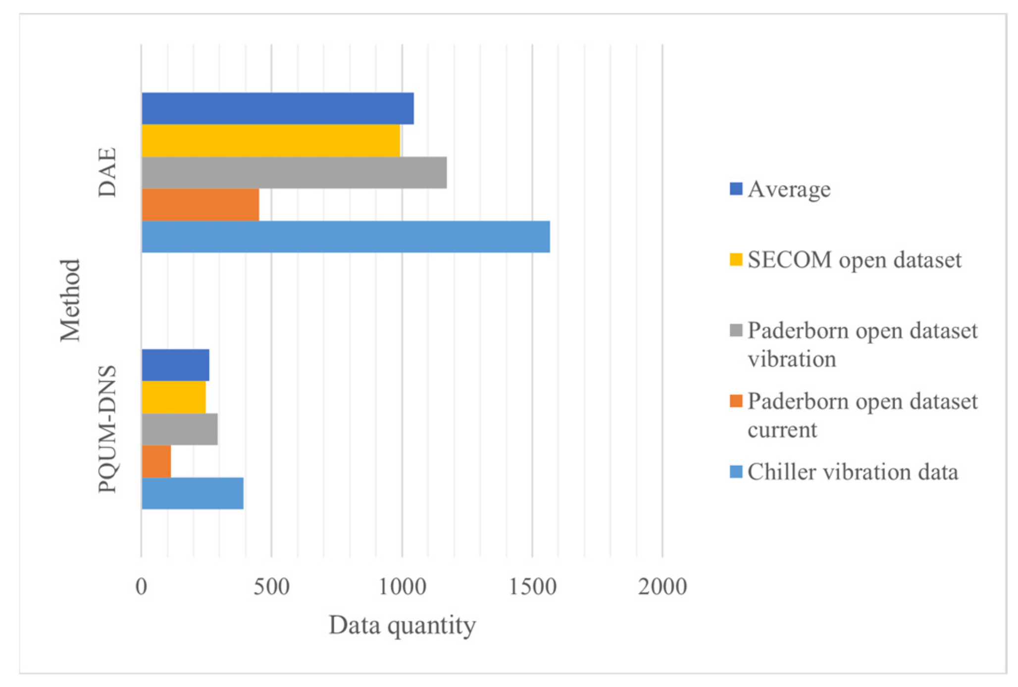
| Data quantity | 392 | 113 | 293 | 248 | 262 | |
| DAE | ||||||
| AUC (%) | 99.99 | 97.03 | 99.73 | 66.14 | 90.73 | |
| Data quantity | 1569 | 452 | 1172 | 993 | 1047 | |
| Improvement | ||||||
| AUC Increase (%) | 0.00 | −4.3 | 0.07 | 2.83 | −0.35 | |
| Data quantity Decrease (%) | 75.02 | 75 | 75 | 75.03 | 75.01 | |
| RMSE | |||||
|---|---|---|---|---|---|
| Algorithm | Chiller Vibration Data | Paderborn Open Dataset Current | Paderborn Open Dataset Vibration | SECOM Open Dataset | Average |
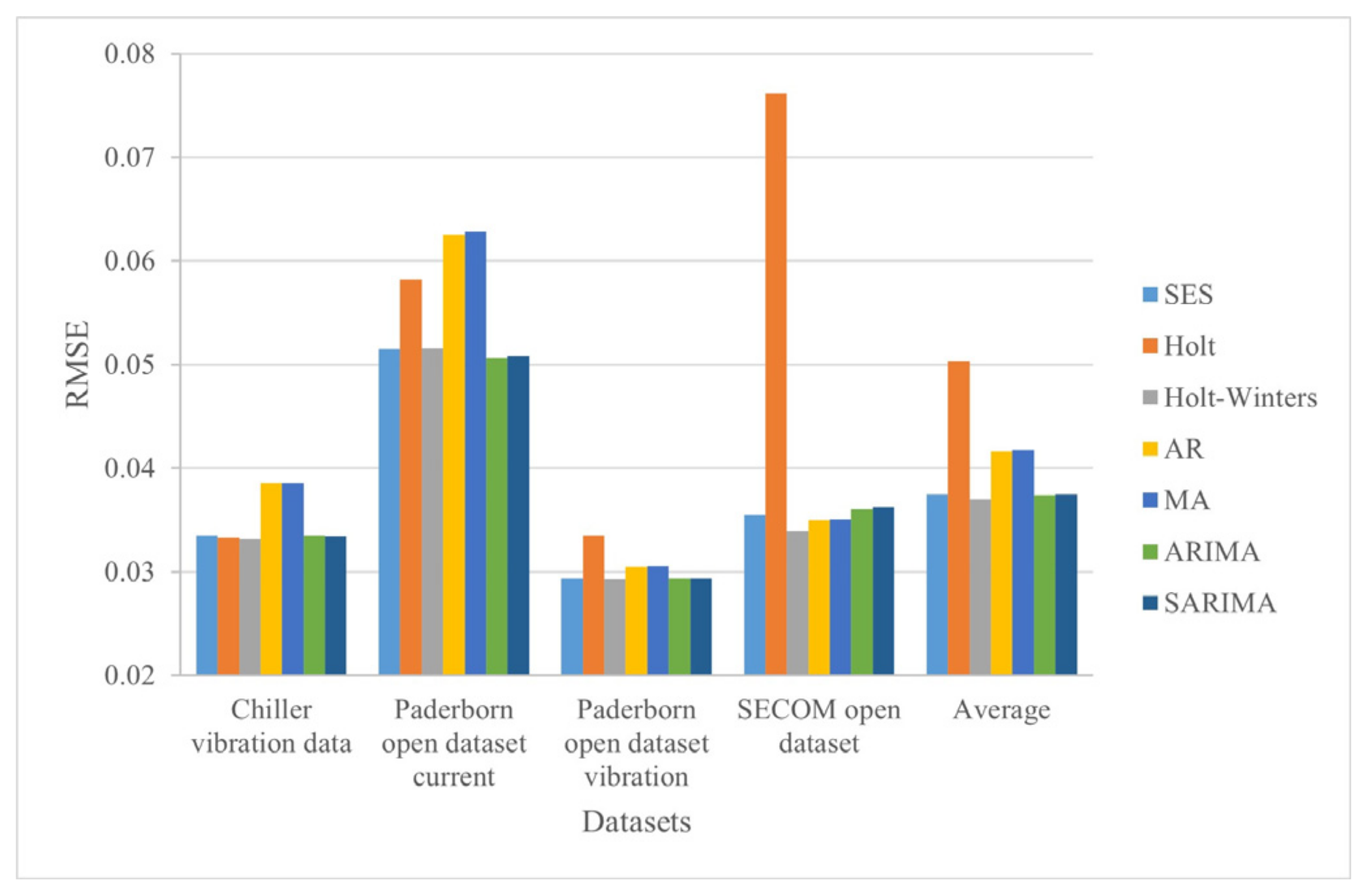
| SES | 0.03350 | 0.05153 | 0.02934 | 0.03547 | 0.03746 |
| Holt | 0.03330 | 0.05824 | 0.03348 | 0.07614 | 0.05029 |
| Holt–Winters | 0.03315 | 0.05161 | 0.02928 | 0.03395 | 0.03700 |
| AR | 0.03855 | 0.06250 | 0.03052 | 0.03500 | 0.04164 |
| MA | 0.03853 | 0.06289 | 0.03057 | 0.03505 | 0.04176 |
| ARIMA | 0.03349 | 0.05062 | 0.02933 | 0.03606 | 0.03737 |
| SARIMA | 0.03347 | 0.05088 | 0.02932 | 0.03626 | 0.03748 |
| Retraining | |||||
|---|---|---|---|---|---|
| Chiller Vibration Data | Paderborn Open Dataset Current | Paderborn Open Dataset Vibration | SECOM Open Dataset | Average | |
| PQUM-DNS | |||||
| Retraining data quantity (fine-tune) | 586 | 54 | 50 | 248 | 235 |
| AUC | 99.99 | 94.68 | 99.99 | 62.6 | 89.32 |
| DAE | |||||
| Retraining data quantity | 2346 | 219 | 204 | 993 | 941 |
| AUC | 99.99 | 96.17 | 99.99 | 66 | 90.54 |
| Improvement | |||||
| Retraining data quantity decrease | 75.02 | 75.34 | 75.49 | 75.03 | 75.07 |
| AUC increase | 0.00 | −1.49 | 0.00 | 5.15 | 1.35 |
| Model Size | |||||
|---|---|---|---|---|---|
| Chiller Vibration Data | Paderborn Open Dataset Current | Paderborn Open Dataset Vibration | SECOM Open Dataset | Average | |
| PQUM-DNS | |||||
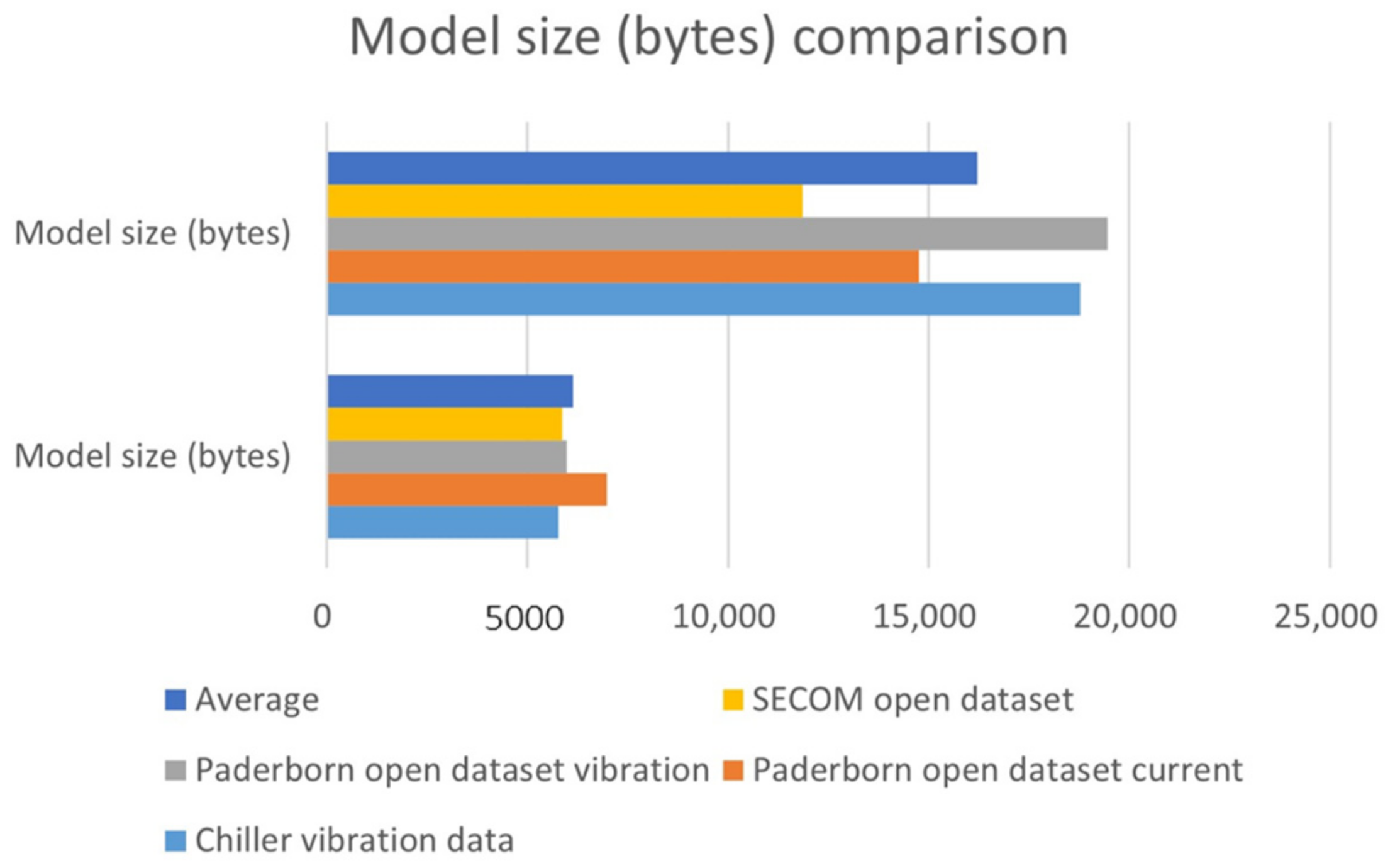
| Model size (bytes) | 5776 | 6969 | 5973 | 5866 | 6146 |
| AUC | 99.31 | 93.16 | 99.34 | 69.69 | 90.38 |
| DAE | |||||
| Model size (bytes) | 18767 | 14765 | 19466 | 11866 | 16216 |
| AUC | 99.31 | 93.16 | 99.34 | 69.69 | 90.38 |
| Improvement | |||||
| Model size decrease | 69 | 53 | 69 | 51 | 60 |
| AUC increase | 0.00 | 0.00 | 0.00 | 0.00 | 0.00 |
Disclaimer/Publisher’s Note: The statements, opinions and data contained in all publications are solely those of the individual author(s) and contributor(s) and not of MDPI and/or the editor(s). MDPI and/or the editor(s) disclaim responsibility for any injury to people or property resulting from any ideas, methods, instructions or products referred to in the content. |
© 2024 by the authors. Licensee MDPI, Basel, Switzerland. This article is an open access article distributed under the terms and conditions of the Creative Commons Attribution (CC BY) license (https://creativecommons.org/licenses/by/4.0/).
Share and Cite
Yu, Y.-C.; Yang, S.-R.; Chuang, S.-W.; Chien, J.-T.; Lee, C.-Y. Pruning Quantized Unsupervised Meta-Learning DegradingNet Solution for Industrial Equipment and Semiconductor Process Anomaly Detection and Prediction. Appl. Sci. 2024, 14, 1708. https://doi.org/10.3390/app14051708
Yu Y-C, Yang S-R, Chuang S-W, Chien J-T, Lee C-Y. Pruning Quantized Unsupervised Meta-Learning DegradingNet Solution for Industrial Equipment and Semiconductor Process Anomaly Detection and Prediction. Applied Sciences. 2024; 14(5):1708. https://doi.org/10.3390/app14051708
Chicago/Turabian StyleYu, Yi-Cheng, Shiau-Ru Yang, Shang-Wen Chuang, Jen-Tzung Chien, and Chen-Yi Lee. 2024. "Pruning Quantized Unsupervised Meta-Learning DegradingNet Solution for Industrial Equipment and Semiconductor Process Anomaly Detection and Prediction" Applied Sciences 14, no. 5: 1708. https://doi.org/10.3390/app14051708
APA StyleYu, Y.-C., Yang, S.-R., Chuang, S.-W., Chien, J.-T., & Lee, C.-Y. (2024). Pruning Quantized Unsupervised Meta-Learning DegradingNet Solution for Industrial Equipment and Semiconductor Process Anomaly Detection and Prediction. Applied Sciences, 14(5), 1708. https://doi.org/10.3390/app14051708