Article

Genetic Multi-Objective Optimization of Sensor Placement for SHM of Composite Structures

1
Department of Fundamentals of Machinery Design, Faculty of Mechanical Engineering, Silesian University of Technology, Konarskiego 18A, 44-100 Gliwice, Poland
2
Institute of Materials and Structures, Riga Technical University, Kipsalas iela 6A, LV-1048 Riga, Latvia
*
Author to whom correspondence should be addressed.
Appl. Sci. 2024, 14(1), 456; https://doi.org/10.3390/app14010456
Submission received: 28 November 2023 / Revised: 27 December 2023 / Accepted: 3 January 2024 / Published: 4 January 2024

Abstract

:
Increasingly often, due to the high sensitivity level of diagnostic systems, they are also sensitive to the occurrence of a significant number of false alarms. In particular, in structural health monitoring (SHM), the problem of optimal sensor placement (OSP) is appearing due to the need to reach a balance between performance and cost of the diagnostic system. The applied approach of considering nondominated solutions allows for adaption of the system parameters to the user’s expectations, treating this optimization problem as multi-objective. For this purpose, the NSGA-II algorithm was selected for the determination of an optimal set of parameters in the OSP problem for the detection of delamination in composite structures. The objectives comprise minimization of type-I and type-II errors, and number of sensors to be placed. The advantage of the proposed approach is that it is based on experimental data from the healthy structure, whereas all cases with a presence of delamination were acquired from numerical experiments. This makes it possible to develop a customized SHM system for the arbitrary location of damage.

1. Introduction

Structural health monitoring (SHM) became a paradigm in the operation of numerous structures and transport means, especially in civil and mechanical engineering, due to the ability to continuously evaluate structural conditions based on measured response and building prognostic models based on this. Currently, SHM is incorporated into the latest design and operation concepts, such as condition-based maintenance (CBM), the philosophy used in aviation, where maintenance is scheduled according to the current condition of the structure only [1,2]. SHM is also an integral part of the newest solutions in civil engineering, such as building information modelling (BIM) [3,4] and the concept of digital twins [5], where it plays a crucial role in the acquisition and management, being the main source of data for the evaluation of structural condition. Regardless of the advancement of the mentioned concepts and approaches based on them, there are still unsolved problems influencing their performance. One of these problems is an appropriate sensor placement that determines the effectiveness of the condition evaluation of a tested structure. It is especially important in the case of SHM systems based on modal analysis, one of the oldest and most widely used approaches in both civil and mechanical engineering [6]. Recent studies of the authors [7,8] demonstrated the need for the application of an advanced machine-learning approach for this task to find a balance between the performance and cost of an SHM system.
There are a plenty of different optimal-sensor-placement (OSP) strategies for SHM. A systematic review on different approaches can be found in [9,10,11]. From these optimization strategies, one group is of sequential-based sensor placement strategies where subsequent steps are based on sequentially eliminated sensor locations that contribute less to the objective functions [10,12] or otherwise by adding sensor locations that enhance the value of the evaluation function [10,13]. Another group are simple or metaheuristic optimization strategies such as greedy algorithms [14], and bioinspired e.g., evolutionary, ant colony, particle swarm, or physically inspired e.g., simulated annealing algorithms [10]. Among the above meta heuristics, evolutionary methods have become evident [10]. These algorithms can be easily customized to the needs of the optimization problem because the objective function can be independently constructed without the need for reconfiguration of the optimization routine, similarly to other heuristic approaches. The objective functions can be built based on classical objectives, e.g., Fisher information matrix (FIT), mutual information (MI), etc., [10] as well as based on outcomes of the SHM system [9] which allows for building different optimization strategies. Increasingly often, different cost functions are taken in order define objective of SHM with an OSP problem. This requires defining of the multiterm weighted objective function or the necessity to build an appropriate aggregation operator [7]. Because in OSP various evaluation functions can be considered and for the SHM systems the performance and costs are counterparts [9], the multi-objective optimization strategies have been recognized as useful strategies. In [15], a decision-making multi-objective optimization based on a particle-swarm algorithm was used. The authors have used a minimum dependency based on Modal Assurance Criteria (MAC), minimum of redundancy based on similarity measure, and the maximization of signal-quality strength as a multi-objective. The obtained Pareto front solution was filtered using the decision-making membership faction to select a subset of obtained solutions. Another study, shown in [16], was based on multi-objective genetic optimization with the application of two objectives using modal shapes. One of the objective was used to compare the modes of the structure amongst themselves, and the other was used to compare the modes of the same structure in two different configurations. The authors also showed comparison of the multi-objective approaches with a single-objective approach and sequential-based sensor-placement strategies, indicating robustness of the sensor networks selected using the multi-objective approach for damage detection of civil construction. Another case study with multi-objective optimization of sensor placement on a composite rotor blade is presented in [17]. The objective function is based on the minimalization of the sensor number and, simultaneously, the minimalization of the error between the reconstructed real mode and the mode based on the information from the candidate sensor networks. Another study [18], presents multi-objective optimization with the combination of maximization of the nominal performance that could be defined using the mean and maximum of MAC, the conditional number, or the effective independence and minimalization of the data uncertainty.
Many of the above-mentioned multi-objective-optimization problems use different algorithms; most of them are dominance-based methods based on popular NSGA-II [17,18,19,20]. This algorithm is often used as long as no more than three objectives are taken into account [21,22]. There are also decomposition-based methods which decompose multi-objective problems into a set of single-objective problems. For instance, Downey et al. [23] presented a bi-optimization objective function based on the accuracy of the strain-map reconstruction based on the optimal-sensor-placement network. They used the concept of minimalization of type-I and type-II errors of the SHM system assuming that these errors can be reduced by minimizing the mean absolute error between the real system and estimated strain map response and by minimalizing the maximum difference between them. It should be noted that the use of multi-objective optimization is an important direction in developing OSP strategies in SHM systems.
In this study, the SHM system is based on the classification-of-information system, which allows to estimate the sensitivity and specificity of damage recognition. These characteristic features, together with the number of used sensors, are taken as individual objectives in the multi-objective optimization of sensor placement. The outcomes are presented as Pareto solutions which, linked to design variables, allow the user to obtain required performance and costs of an SHM system. This is an ongoing study within a series of previously performed studies [7,8] with a general focus on development of a customizable SHM system with a trade-off between performance and cost effectiveness.

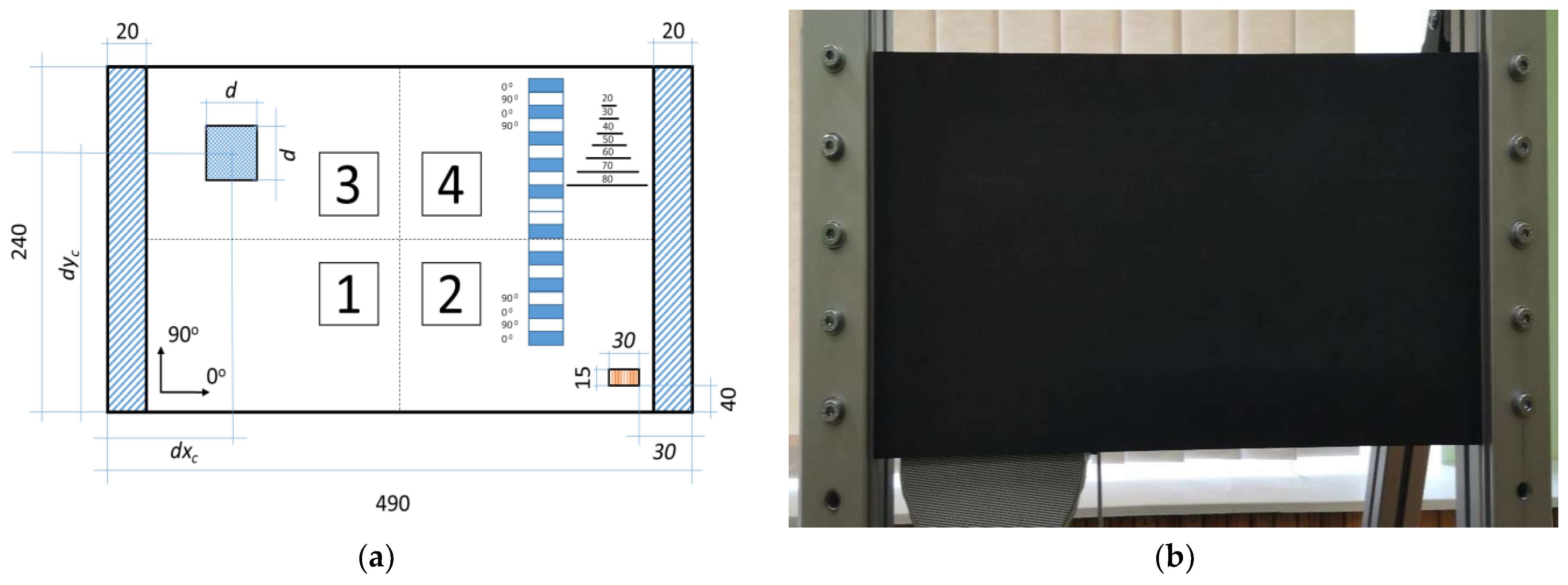
2. Tested Structure and Experiments

2.1. Parameters of the Tested Structure

The structure considered in this study to test the developed OSP approach is a carbon-fiber-reinforced polymeric (CFRP) composite plate with the dimensions of 490 × 240 mm, thickness of 1.84 mm, and the following stacking sequence: (0/90)5s (see Figure 1a). In the study, the healthy plate was considered as a reference for building the numerical models described in the next subsection. The detailed description of the manufacturing process and material properties of this plate are presented in [7].
The plate was fixed on the shorter side to the aluminum frame at a distance of 20 mm from the edge using screws located with a distance of 50 mm on the clamped sides and a tightening torque of 20 Nm. The plate was then subjected to mechanical excitation using the Penton CAD10T/EN loudspeaker (Worthing, UK) using the periodic chirp signal in the bandwidth of 0 ÷ 625 Hz with a resolution of 0.195 Hz (see Figure 1b).
The measurements of a structural response were performed on a defined grid of 25 × 13 equidistantly spaced measurement points using a Polytec® PSV-500-3D scanning laser vibrometer (Waldbronn, Germany) with three averaging cycles to improve the accuracy of the measurements. During measurements, the vibration velocity in the defined measurement points was acquired. Details on the experimental setup are provided in [7]. As a result of the performed measurements, the structural response of a plate was acquired in the form of a frequency-response function (FRF). The natural frequencies determined from the modal analysis are presented in Table 1.
To determine the strain values in both directions for the tested plate, Sx and Sy, respectively, the transverse displacements w were considered. Further, from transverse displacements smoothed using the least squares linear regression, the strain fields were determined. Each smoothed value is determined using the adjacent data points. The strain value maps were normalized in such a way that the largest value was assigned to a unit and the remaining values were scaled relative to the maximum value. The deformation values on the plate surface in appropriate directions are calculated using the following formula:
S x ( i , j ) = 2 w x 2 ( i , j ) ·   1 2 h ;   S y ( i , j ) = 2 w y 2 ( i , j ) ·   1 2 h ,
where h is the thickness of the plate.

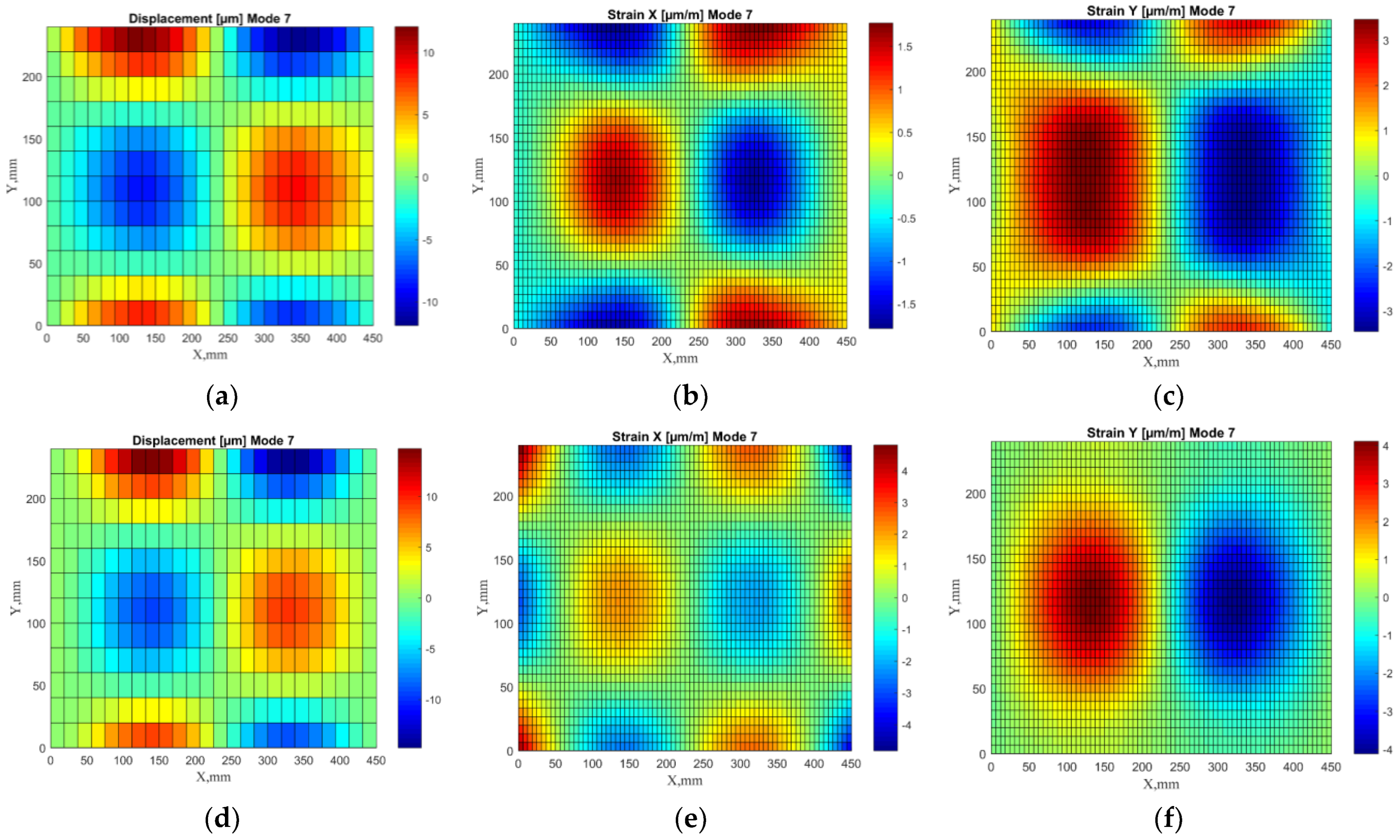
2.2. Numerical Experiments

Data for the intact plate were collected from the laboratory experiment. Additionally, numerical experiments have been performed to collect data from various conditions of structural damage. In order to develop a system for recognizing other health conditions (the presence of delamination in this case), it was necessary to supplement the set of learning examples with data coming from damaged conditions. For this purpose, it was decided to supplement these data using an appropriately tuned numerical model. The model was tuned based on data for the intact condition, and then, after an appropriate level of compliance between the model and the experimental data was reached, the condition with the presence of delamination was simulated. The model developed in this way made it possible to obtain a set of learning examples covering damage conditions. The detailed description of the definition of the numerical model and performing numerical simulations as well as further processing of data was presented in the previous work [7].
The parameters and constraints of the model were assigned to be consistent with the physical tested plate. Each layer of the composite plate is represented by a single element throughout the thickness. Numerical modal analysis was used to determine the first seven dominated eigenvalues and eigenvectors. To obtain the strain values, the absolute values of the transverse displacements were normalized in descending order. The strain values were calculated according to Formula (1). To obtain a denser mesh, the strain fields were smoothed using regression analysis. An example comparison of experimental and numerical transverse displacements shapes and adequate strain shapes is shown in Figure 2.

3. Multi-Objective Optimization

3.1. OSP Problem

The primary goal of OSP is to localize the positions of the sensors in order to collect relevant information about the analyzed structure. This information, together with the available knowledge about the observed structure, allows for estimating its health condition which is, in turn, one of the main objectives of an SHM system. Usually, the process of determining sensor placement can be a part of the design of an SHM system [20]. This is often preceded by the evaluation of the structural characteristic and dynamics of the structure and also the selection of appropriate sensor types. The selection of the sensor type and the evaluation of the dynamic characteristic of the composite plate was a part of the research in [7], and is based on the application of strain gauges oriented horizontally or vertically to monitor modal strain of the composite plates. Usually, the next step comprises the necessity of sensor placement. This optimal placement strongly depends on the objective function of the unconstrained or constrained optimization process. There are many objective functions widely used for that purpose, e.g., a function based on Fisher matrix indices [24,25], MAC [20,24], condition number [24], modal kinetic-energy-based index [26], and many others, e.g., [9]. Most of them are mainly based on the assumption of widely understood criteria of independency, which allow one to select these locations of the sensors with the minimum redundancy of the captured data. In addition to that, from the perspective of the effectiveness of the whole SHM system, including the OSP problem, information on the health condition of the analyzed structure is the primary outcome of any SHM system.
Taking the above into account, the spatial placement of the sensor network can be based on the final evaluation of the SHM system, such as the effectiveness of a properly recognized heath condition of the structure. This allows one to establish adequate input to design parameters of the optimization process such as number of sensors, number of analyzed modes, etc., and to link them directly to the final effectiveness of the SHM system instead of using intermediate criteria such as statistical independency criteria, mutual information criteria, and any others [20,24,25,26].
In this study, the minimalization of the type-I and type-II errors were taken separately as the main criteria for the evaluation of the effectiveness of the SHM system [10,23,27]. The minimalization of type-I error allows for increasing the specificity of the system leading to a lower number of false alarms. The minimalization of the type-II error allows one to enhance the sensitivity of the system in accurate detection of the health condition minimizing any misses in the condition recognition. Keeping both of these criteria in balance requires a trade-off and is crucial for designing SHM systems. For instance, too-high sensitivity may lead to low specificity with a high number of false alarms, which may lead to information overload of the human operator of the SHM system. On the other hand, maintaining high specificity may lead to poor performance in the recognition of all faulty states of the structure. In the paper [23], it was shown that both sensitivity and specificity are often opposite counterparts in classification problems. Both types of errors are also naturally opposite to the minimalization criteria of the number of sensors used. Usually more relevantly selected and placed sensors lead to minimization of the type-I and type-II errors, but are more costly and require more data to analyze.
In many cases, the designer of the SHM system can be interested in solutions with enhanced sensitivity rather than false-alarm avoidance. In this case, a weighed objective function in multi-objective optimization allows for analysis of a specific region of the Pareto front, biasing the search towards a solution that optimizes weighed objective function. In this study, for the purpose of not losing the wider diversity of Pareto front solutions, no weights have been considered, leaving the designer to select results from the wider range of possible solutions and its design parameters.
Taking all of these multiple conflicting objectives into account, the multi-objective optimal-sensor-placement problem can be defined as follows, where the objective functions can be represented as
f 1 x 1 , x 2 , x 3 = F P ( x 1 , x 2 , x 3 ) T N ( x 1 , x 2 , x 3 ) + F P ( x 1 , x 2 , x 3 ) ,
f 2 x 1 , x 2 , x 3 = F N ( x 1 , x 2 , x 3 ) T P ( x 1 , x 2 , x 3 ) + F N ( x 1 , x 2 , x 3 ) ,
f 3 x 1 = n x x 1 + n y ( x 1 ) ,
where, f 1 ,   f 2 ,   f 3 are objective functions associated with the minimalization of type-I error, type-II error, and the minimalization of the total sensor used, respectively. The vector of x = x 1 . x 2 ,   x 3 is a vector of design variables, where x 1 represents the total number of sensors, x 2   is number of used shape modes, and x 3 indicates the required minimal distance between the sensors measuring the strain displacements in the same direction, because the modal modes, especially for the healthy condition, are symmetrical. The minimum required distance allows for maintaining the spread of the sensors at the surface of the plate avoiding placing them in the same quadrant. FP, TN, FN, and TP correspond to false-positive, true-negative, false-negative, and true-positive cases, respectively [25]. Because the proposed SHM is a classification-based information system, these parameters are evaluated using classification statistics obtained using k-fold validation based on classification-error statistics [9,25]. The n x , n y   corresponds to the number of strain sensors used for measuring along the x and y direction, respectively. Finally, multi-objective optimization is defined to minimize
F x = m i n ( f 1 ,   f 2 ,   f 3 ) ,
subject to
3 x 1 10   ;     2 x 2 7   ;   120   x 3 200 ,
d s x i x , y , s x j x , y x 3 ;   d s y i x , y , s y j x , y x 3 ;   f o r   i j ,    
where s x i ( x , y ) , s y i x , y are the positions of the i-th and j-th strain gauges oriented horizontally, s x i , and vertically, s y i , at the coordinates x , y , and d is the Euclidean distance between the considered sensors. The range from 2 up to 10 sensors was used to maintain the consistency of this paper with previous studies [7]. The lower limit of 2 sensors requires the use of at least one sensor in every X or Y direction. The upper boundary has been selected based on the limited number of channels in our measurement path presented in [8]. The number of modes was also selected according to the number of modes used in previous research [7]. The upper boundary of the number of modes was limited to seven most-dominated modes in the frequency-response function; therefore, the 7th, 5th, 6th, 9th, 4th, 10th, and 8th mode from Table 1. were taken into account. The last mode from this set, the 8th mode, has about 10% of the energy of the highest mode. Other modes in the considered band rate have less than or equal to 5% of the energy in comparison to the most dominated mode. The value of minimum required distance was established based on the occurrence of the symmetric modes’ shapes of which the strain values are the same (for the healthy condition of the plate) in four imaginary quadrants of the plate visible in Figure 1a. To force the placing sensor in separate imaginary quadrants, this value of 120 mm was selected as the low boundary. A similar approach was used in the study [7]. On the other hand, the upper limit of the required distance between the sensors was also limited to avoid considering unfeasible solutions where a large number of sensors with the same orientation could not be placed in the limited plate size.
To limit the number of possible solutions, it has been assumed that the position of the sensors are assigned to the closest node of the virtually superimposed grid on the composite plate, where nodes are vertically and horizontally spaced with the distance of 5 mm:
x , y N   |     x i x j = 5 k ,   y i y j = 5 m     k , m N
Due to the dimensions of the side clamps of the considered composite plate and the size of strain gauges, the coordinate values are limited to the following limits: 20 x 470   a n d   5 y 235 . The number of possible combinations of sensor placement, excluding constraint of the required distance between sensors is still huge and comprises, e.g., for three sensors 1.18 × 10 10 , candidate solutions.
The multi-objective approach allows one to obtain decision variables of an SHM system to be independent of any weighed multi-objective function approach, which usually is difficult to determine at the early stage of the designing process. For SHM design purposes, the proposed multi-objective approach should return nondominated solutions using the approximation of the Pareto front for the considered individual objectives. Nondominated solutions obtained in this way give an opportunity for the designer to select appropriate parameters of the SHM system, adjusting it to the appropriate sensitivity level of fault recognition and at the same time keeping the appropriate level of false alarms and considering the appropriate cost of the system with the number of sensors used.

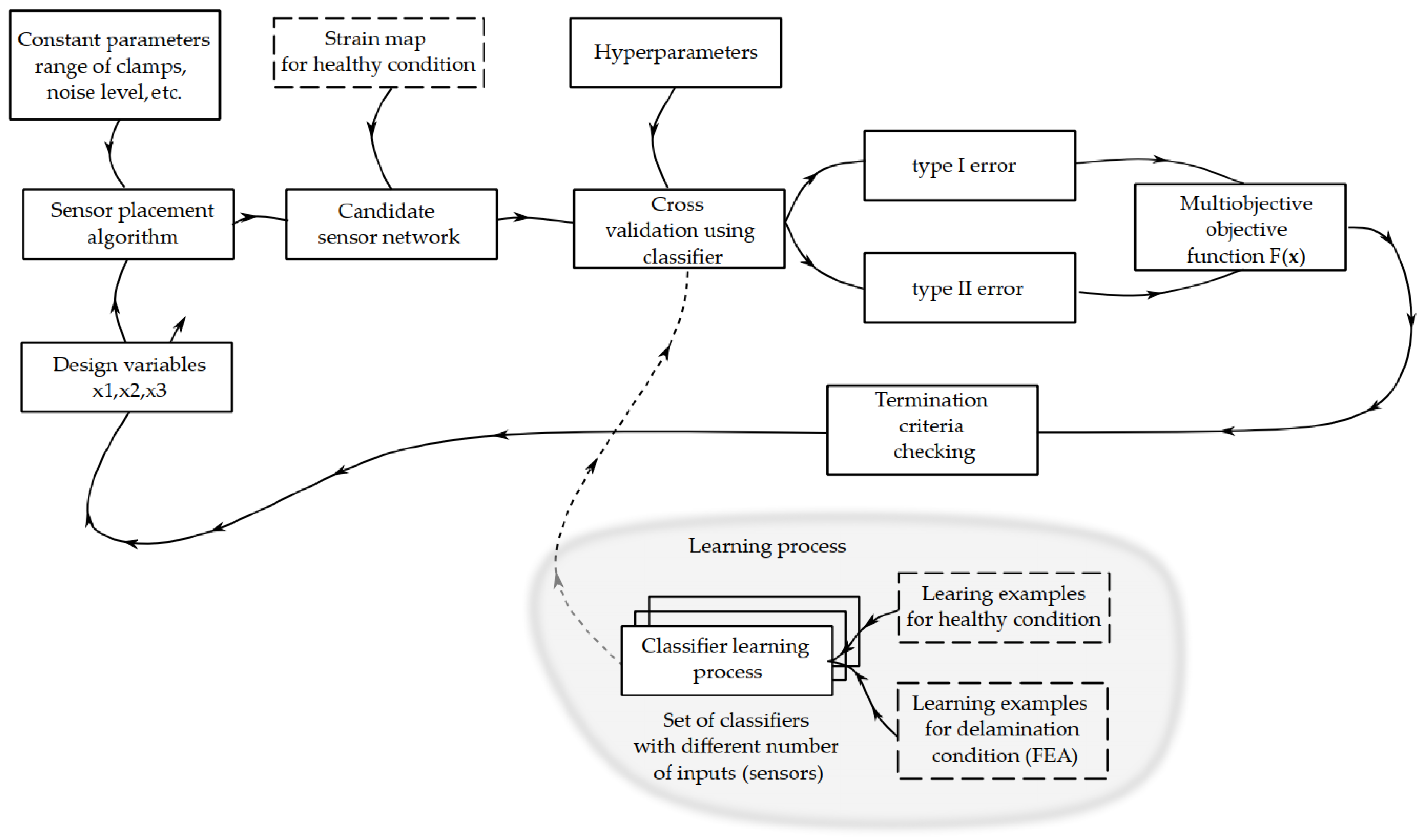
3.2. General Optimization Procedure

To estimate individual objectives of F x , the SHM effectiveness through the estimation of classification performance statistics need to be completed. For this purpose, a classifier should be prepared that takes information on the strain values for the given coordinates according to the sensor’s network placement, and returns the information about the health condition of the composite plate. Separately, to avoid using the coordinates of the location of the sensors as design variables, the appropriate method of sensor placement was used internally in this proposed optimization procedure. This allows one to take advantage of the available knowledge on the effectiveness of the selected sensor-placement algorithm used for the composite plate based on the results obtained in [7].
The general optimization procedure is based on the application of a heuristic approach with elitist modification of the NSGA-II algorithm [18,20,28,29,30,31]. The algorithm allows approximation of the Pareto front which represents the equivalent trade-off between considered objectives f 1 ,   f 2 ,   f 3 . In this paper, the optimization framework launch execution of other processes such as OSP and validation of classification. The general scheme of the optimization process is shown in Figure 3.
The NSGA-II executes the process of multi-objective optimization by defining an initial and any after generation, where individuals represent candidate sensor networks. These sensor networks are generated using the sensor-placement method based on selected design parameters and available strain maps for different shape modes obtained experimentally, according to [7], for the heathy condition of the composite plate. During the process of optimization, some of the parameters are treated as constant parameters, among others, they include the clamping area of the composite plate, where placing sensors is not possible. Another constant parameter is the relative additive noise level used in data augmentation for the purpose of obtaining balanced dataset for learning of the classifiers.
In this research, one of the algorithms for sensor placement shown and evaluated in the paper [7] was used. This algorithm is based on the selection of the position of the sensor candidates on the rank defined on the basis of the sum of values of the mode shapes for individual coordinates. Initially, the mode shapes are ordered according to their higher dominance in frequency-response function shown in Table 1. Next, individual strain maps of selected modes are normalized from 0 to 1, assigning 1 to the highest strain value. Then, the sum of the strains of selected modes is performed, and the strain values in the x and y direction are organized separately as vectors of values in descending order [7,8]. Afterwards, based on this order, the sensors are sequentially placed in the coordinates, which corresponds to the highest value in the mentioned vector, taking into account other requirements such as maintaining the required distance between sensors, etc. The effectiveness of this algorithm was compared with other algorithms, among others, with a modified Effective Independence Method [12]. In this comparison, we also took into account the influence of the noise level on the accuracy of damage detection. More details can be found in [7].
In this study, the sensor network obtained using the above algorithm is mainly evaluated using the prepared classifier, which is validated using k-fold cross-validation. The results of this validation make it possible to compute the objective function f 1 ,   f 2 , which represents the number of type-I errors and type-II errors. This allows one to compute a multi-objective function for the individuals in the considered generation. The selection process of individuals for the next generation is performed using the tournament selection [23] with a fraction value of 0.8. During the creation of offspring generations, the mutation operator that allows individuals to generate feasible values that meet the bound constraints shown in Equations (5) and (6) was used [32]. The one-point crossover operation on the basis of an intermediate combination [32] was used.
In the process of the optimization evaluation, the following termination criteria were used. If the spread distance of the solutions across the Pareto front changes less in subsequent iterations than an established tolerance, the optimization process should stop. Otherwise, if the limited number of generations will be computed, the process may stop as well. Due to the heuristic characteristics of the conducted optimization, e.g., making the process of optimization independent of the process of the initial generation of the design variables, the process was repeated several times. In addition to the optimization process, the obtained Pareto front was evaluated using the standard deviation of the Pareto distance [28]—a standard deviation of distances between two closest neighbors for nondominated solutions. In these calculations, the dominated solutions at the ends of the Pareto fronts are omitted. The second evaluation parameter was defined as the spread distance, which takes the standard deviation of the Pareto distance as an internal parameter. Apart from the Pareto distance [28], the spread distance [28] allows one to estimate the change of the Pareto fronts in a subsequent iteration of the optimization process. The lower the value, the more equally can distributed solutions on the Pareto front be reached.
The evaluation of the current health condition of the analyzed plate is based on the observed relevant sensor network, and based on the appropriate information obtained from the acquired knowledge about the dynamic modal behavior of the composite plate for healthy and damage conditions. This approach requires an appropriate representation of knowledge, which, in this case, takes the form of an intrinsic mathematical representation of the trained k nearest-neighbor classifier (k-NN).
For the purpose of the estimation of hyperparameters, a separated validation dataset was prepared. This validation set consisted of 54 sensor networks obtained individually for all combinations of the number of sensors from 2 to 10 and the number of modes from 2 to 7. These sensors positions were established based on the criteria shown in paper 7. These solutions are dominated solutions used only for the purpose of hyperparameters’ selection. Every dataset for every sensor network contains a set of 2560 validation examples. The Bayesian optimization in the space of the considered hyperparameters was performed using Matlab© fitcknn routine. The objective function used for this purpose was the loss function estimated as 1-classification accuracy. In order to maintain good generalization properties of the classifier and to avoid overlearning, the estimated nearest classifier numbers were selected based on the criteria that this hyperparameter does not lead to a higher difference than 1% of the loss function between the best selection indicated by the routine, usually with a high number of neighbors and one that is selected manually with a very limited number of nearest neighbors. The analysis indicated that squared Euclidean, Minkowski, Euclidean, Chebyshev, Cityblock, and Mahalonobis do not indicate any significant differences between classification accuracy (more than 5%).
The selection of the hyperparameters mentioned above allows us to estimate the hyperparameters separately for the set of classifiers with different input numbers (number of sensors). Finally, the squared Euclidean distance with four nearest neighbors and inverse distance weighing were efficient to obtained high-accuracy classifiers for the set of used classifiers. For data sets that contain information from more than five modes, even three or two nearest neighbors can be applied without loss of classification accuracy.
The general optimization procedure described in this section was implemented in the Matlab© 2023a release (MathWorks Inc., Natick, MA, USA) using k-NN and NSGA-II Matlab built-in algorithms.

3.3. Data Preparation

The process of multi-objective optimization requires preparing a high-accuracy trained classifier which allows the evaluation of the value of the multi-objective function for all individuals. In this study, the classifiers are learned and validated during every iteration of the optimization procedure for the known number of inputs (sensor numbers) and selected strain modes. Due to the stochastic nature of the selection of the subset of the data sets for learning and validation for the same set of design variables, small differences can be observed for the same value of the input variable vector as a result of this stochastic nature. To decrease the variability of the results of the type-I and type-II errors due to the mentioned stochastic nature, a ten-fold cross-validation procedure was used to evaluate the classification statistics.
The proper evaluation of the objective function using type-I and type-II errors requires also a balanced data set preparation. For this purpose, the learning data set was augmented using replication of the learning examples with additive noise with normal distribution. The additive noise of the percentage k is defined as of 95% probability with the value ε falling within the range of ε [ a , + a ] , which can be written as follows:
Φ μ , σ 2 a Φ μ , σ 2   a = 95 % ,
where Φ μ , σ 2 is a cumulative normal distribution with the mean μ and the standard deviation σ 2 . This requires the estimation of the standard deviation σ 2 of the zero-mean normal distribution based on the following equality equation:
Φ 1 97.5 % ;   σ 2 Φ 1 2.25 ;   σ 2 = 2 a
where Φ 1 is the inverse cumulative normal distribution of the zero mean estimated at the boundaries of the 95% probability interval, and σ 2 is seeking standard deviation. Solving Equation (8) provides the required value for the standard deviation. In this case, for normalized values of strain maps, a 5% normal additive noise has a standard deviation of 2.551 × 10 2 .
The noise level was established on the basis of the initial evaluation of an accuracy of the damage recognition on the basis of a random subset of input variables with a lower number of sensors and a lower number of modes. The goal of the selection of this noise level was to select the highest value of the noise level to obtain the highest possible generalization properties of the classifier, which still guarantee obtaining a satisfactory level of damage recognition. For this purpose, a five-fold cross-validation procedure was used for the selected subset of input variables with different numbers of sensors, modal shape numbers, and different noise levels from 2 up to 5%. As a satisfactory level of the classifier validation accuracy, at least 95% of classification accuracy [25] was used. It has been observed that for the first three mode shapes and two sensors with a level of 5% of additive random noise, the validation accuracy leads to 95.6%. For other cases and lower noise levels, the validation outcome resulted in higher accuracy. Due to this, the noise level of 5% was attributed as a noise level in the augmentation process of a leaning dataset. The idea of using a high possible noise level results from using numerous numerical cases in the learning examples to maintain high generalization properties of the used classifiers.

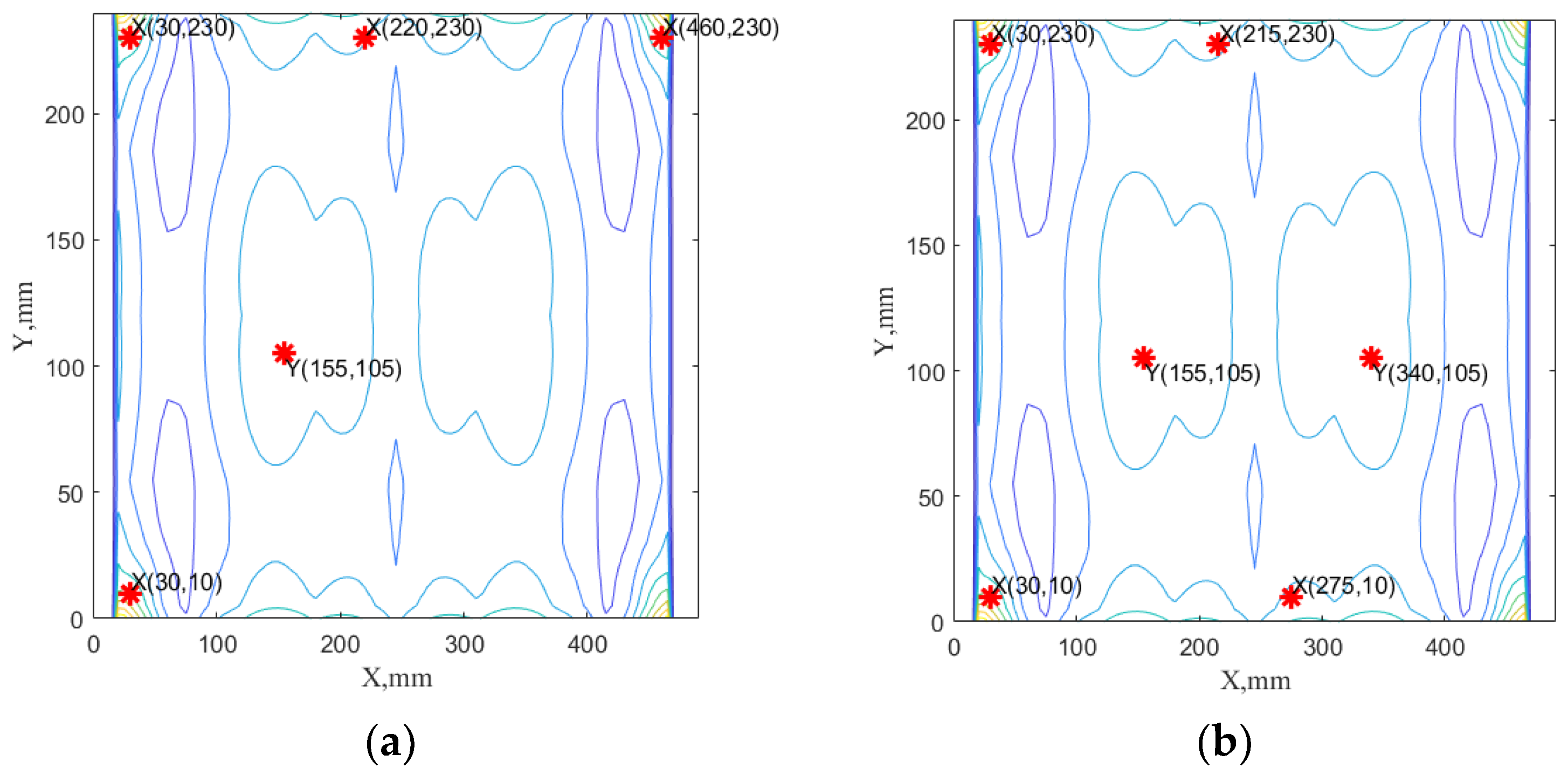
3.4. Optimization Results

The results of the optimization process allows for estimating the approximation of the Pareto front for the multi-objective function shown in Equation (5). Finally, the front is represented by 38 solutions. The optimization process was terminated, since the average change in the spread of the Pareto solutions was less then 10 4 . The standard deviation of an average distance for the solution equals 10.41 × 10 2 and the spread distance equals 29.51 × 10 2 . The solutions have been obtained after 51 generations. To avoid the influence of the randomly generated initial population and also to avoid the influence of any other stochastic processes (e.g., a 10-fold validation process), the process was repeated several times. No significant changes have been observed in the repetitions of the optimization process.
Pareto solutions in the multi-objective function domain are shown in Figure 4a. The parameter space can be observed in Figure 4b. Additionally, some projections of the Pareto solutions for type-I and type-II errors are presented separately in Figure 4c and Figure 4d, respectively. In Figure 4c,d, dominated solutions from the results of paper [7] have been added as well. These results have been obtained using the same OSP algorithm for single-objective optimization based on the aggregated t-norm evaluation function presented in [7] and with the constant required minimum distance of 127.5 mm.

4. Analysis and Discussion

The analysis of the obtained results indicates that the process of multi-objective optimization based on Pareto front leads to many nondominated solutions, which allows for binding effectiveness of the SHM system with design variables. Based on this information, the designer of the SHM system may decide on the number of sensors in the individual direction, their placement, and the number of modes, simultaneously, while keeping an appropriate level of sensitivity in the system in damage detection as well as an appropriate level of possible false alarms.
To facilitate the SHM user to make decisions about the characteristic sensitivity, specificity, and the utilized sensor number, the obtained results of optimization can be further postprocessed to support this selection. A common-sense approach that can be used for that purpose is a Pareto principle that 80% of the effects come from 20% causes. Using this principle, the Pareto front solutions have been divided into the following subset:
z A g ( z ) z Z g ( z ) 0.8   f o r   g z = log z + 1   a n d   g ( z 1 ) g ( z 2 ) g ( z n )
where
{ z A   |   z = f 1 + f 2 + α f 3 }   or   { z B   |   z = β f 1 + f 2 } .
Annotation z i represents individual solutions of a Pareto front, g z is the negation transformation function, and z A   represents the subset of Pareto solutions with a cumulative contribution of the top 20% solutions, when all objective functions f 1 , f 2 , f 3 are taken into account, but with limited influence of the number of sensors represented by weight α . Similarly, z B   represents the subset of Pareto solutions with cumulative contribution of the top 20% solutions when the sum of type-I and type-II errors are taken into account, with the limited influence of the type-I error represented by weight β . In the present study, the following exemplary weights were assumed, α = 0.2 and β = 0.5 . These weights can be appropriately estimated for the known costs of sensors and required unbalanced performance toward type-I or type-II errors. The Pareto solutions shown in Figure 4 represented by the magenta-filled circles show the top 20% of solutions for set A, and the green-filled circles show solutions for the weighed sum of the observed type-I and type-II errors represented by set B.
The analysis of Figure 4b together with Figure 4c,d of the obtained results indicates that optimal solutions, which belong to the set A set, require the use of four to six sensors and the first six dominated modes (7th, 5th, 6th, 9th, 4th, 10th). An exemplary sensor network for this subset of possible sensor networks is presented in Figure 5.
In that case, when set B is considered, five to eight sensors are necessary to consider with the use of at least first five to seven dominated modes. This can be observed in Figure 4c,d, and also in Figure 6, where the sum of the errors versus the number of sensors are presented.
The analysis of the design variables of the solutions belonging to set B , shown in Figure 4b. indicates that for six to seven sensors it requires consideration of at least six modes to effectively recognize the healthy conditions of the composite plate. The solution with the minimal error type-II is presented in Figure 7a. This sensor networks consist of seven sensors, five in the x direction and two in the y direction for the required distance of 177 mm and the first five dominated modes (7th, 5th, 6th, 9th, 4th). The exemplary sensor network for solutions of set B is presented in Figure 7.
This case study is based on the experience gathered in the ongoing studies presented in [7,8]. In paper [7], specific optimal-sensor-placement algorithms and different ways of evaluating sensor networks using different aggregated criteria were selected and compared. Additionally, the selected classification models that allow the mapping of signals from sensor networks to the evaluation of the condition of the composite plate were selected and validated. In [8], validation of optimal-sensor-placement networks based on the experimental data was shown. It should be emphasized that the ongoing studies presented in [7,8] were aimed at finding the optimal solutions based on the accuracy of composite-plate state recognition, but the candidate sensor-placement networks were selected based on the intermediate criteria such as Fisher matrix indices, etc. These results are also presented in Figure 4c,d and Figure 6. In the present study, the selection of the optimal sensor network is driven by the evaluation of the SHM system using minimization of type-I and type-II errors and the number of sensors. Comparison of the results shows the advantage of the optimization framework presented in this study over the previous results where the optimal-sensor-network selection was not dependent on the final outcome of the SHM system.

5. Conclusions

This study presents the results of multi-objective optimization of the sensor-placement network evaluated using the effectiveness of the SHM system. This effectiveness was achieved by evaluating the sensitivity to recognize the damage condition of the composite plate and also by minimizing false alarms. Additionally, this evaluation can be completed using the minimization of the sensor number, which allows for finding the trade-off between the cost and performance of an SHM system. A specific genetic approach using NSGA-II allowed for recognizing Pareto front solutions and allowed the designer of an SHM system the opportunity to select appropriate values of design variables. The examples with five, six, and seven sensors in the sensor network were demonstrated as the solutions of the performed optimization in this study. This decision can be taken by directly linking the selected results with the design variables. In this study, a selection of design variables based on the Pareto principle is also proposed.

Author Contributions

Conceptualization, T.R., A.K. and S.R.; methodology, T.R., S.R., A.K. and M.Ś.; software, T.R., M.Ś. and S.R.; validation, T.R. and M.Ś.; formal analysis, T.R. and M.Ś.; investigation, S.R.; resources, S.R.; data curation, S.R., T.R. and M.Ś.; writing—original draft preparation, T.R., A.K. and S.R.; writing—review and editing, T.R., A.K. and S.R.; visualization, T.R., A.K. and S.R.; project administration, S.R.; funding acquisition, S.R. and A.K. All authors have read and agreed to the published version of the manuscript.

Funding

This research was partially funded by the Latvian Council of Science project “Smart Materials, Photonics, Technologies and Engineering Ecosystem” (project No. VPP-EM-FOTONIKA-2022/1-0001).

Data Availability Statement

The data that support the findings of this study are available upon reasonable request. The data are not publicly available due to ongoing research process.

Conflicts of Interest

The authors declare no conflicts of interest. The funders had no role in the design of the study; in the collection, analyses, or interpretation of data; in the writing of the manuscript; or in the decision to publish the results.

References

  1. Tinga, T.; Loendersloot, R. Aligning PHM, SHM and CBM by understanding the physical system failure behaviour. In Proceedings of the PHM Society European Conference, Nantes, France, 8–10 July 2014. [Google Scholar]
  2. Broer, A.A.R.; Benedictus, R.; Zarouchas, D. The need for multi-sensor data fusion in structural health monitoring of composite aircraft structures. Aerospace 2022, 9, 183. [Google Scholar] [CrossRef]
  3. Sadhu, A.; Peplinski, J.E.; Mohammadkhorasani, A.; Moreu, F. A review of data management and visualization techniques for structural health monitoring using BIM and virtual or augmented reality. J. Stuct. Eng. 2022, 149, 03122006. [Google Scholar] [CrossRef]
  4. Fawad, M.; Salamak, M.; Poprawa, G.; Koris, K.; Jasinski, M.; Lazinski, P.; Piotrowski, D.; Hasnain, M.; Gerges, M. Automation of structural health monitoring (SHM) system of a bridge using BIMification approach and BIM-based finite element model development. Sci. Rep. 2023, 13, 13215. [Google Scholar] [CrossRef] [PubMed]
  5. Bado, F.M.; Tonelli, D.; Poli, F.; Zonta, D.; Casas, J.R. Digital twin for civil engineering systems: An exploratory review for distributed sensing updating. Sensors 2022, 22, 3168. [Google Scholar] [CrossRef]
  6. Janeliukstis, R.; Mironovs, D.; Safronovs, A. Statistical structural integrity control of composite structures based on an automatic operational modal analysis—A review. Mech. Compos. Mater. 2022, 58, 181–208. [Google Scholar] [CrossRef]
  7. Ručevskis, S.; Rogala, T.; Katunin, A. Optimal sensor placement for modal-based health monitoring of a composite structure. Sensors 2022, 22, 3867. [Google Scholar] [CrossRef]
  8. Ručevskis, S.; Rogala, T.; Katunin, A. Monitoring of damage in composite structures using an optimized sensor network: A data-driven experimental approach. Sensors 2023, 23, 2290. [Google Scholar] [CrossRef] [PubMed]
  9. Barthorpe, R.J.; Worden, K. Emerging Trends in Optimal Structural Health Monitoring System Design: From Sensor Placement to System Evaluation. J. Sens. Actuator Netw. 2020, 9, 31. [Google Scholar] [CrossRef]
  10. Hassani, S.; Dackermann, U. A Systematic Review of Optimization Algorithms for Structural Health Monitoring and Optimal Sensor Placement. Sensors 2023, 23, 3293. [Google Scholar] [CrossRef]
  11. Wang, Y.; Chen, Y.; Yao, Y.; Ou, J. Advancements in Optimal Sensor Placement for Enhanced Structural Health Monitoring: Current Insights and Future Prospects. Buildings 2023, 13, 3129. [Google Scholar] [CrossRef]
  12. Kammer, D.C. Sensor placement for on-orbit modal identification and correlation of large space structures. J. Guid. Control Dyn. 1991, 14, 251–259. [Google Scholar] [CrossRef]
  13. Azin Mehrjoo, B.; Moaveni, B.; Papadimitriou, C.; Khan, U.; Rife, J. Iterative optimal sensor placement for adaptive structural identification using mobile sensors: Numerical application to a footbridge. Mech. Syst. Signal Process. 2023, 200, 110556. [Google Scholar]
  14. Zhang, B.-Y.; Ni, Y.-Q. A data-driven sensor placement strategy for reconstruction of mode shapes by using recurrent Gaussian process regression. Eng. Struct. 2023, 284, 115998. [Google Scholar] [CrossRef]
  15. Lin, T.-Y.; Tao, J.; Huang, H.-H. A Multiobjective Perspective to Optimal Sensor Placement by Using a Decomposition-Based Evolutionary Algorithm in Structural Health Monitoring. Appl. Sci. 2020, 10, 7710. [Google Scholar] [CrossRef]
  16. Civera, M.; Pecoreelli, M.L.; Ceravolo, R.; Surace, C.; Fragonara, L.Z. A multi-objective genetic algorithm strategy for robust optimal sensor placement. Comput.-Aided Civ. Infrastruct. Eng. 2021, 36, 1185–1202. [Google Scholar] [CrossRef]
  17. de Souza Mello, F.M.; Pereira, J.L.J.; Gomes, G.F. Multi-objective sensor placement optimization in SHM systems with Kriging-based mode shape interpolation. J. Sound Vib. 2024, 568, 118050. [Google Scholar] [CrossRef]
  18. Yang, C.; Xia, Y. Interval Pareto front-based multi-objective robust optimization for sensor placement in structural modal identification. Reliab. Eng. Syst. Saf. 2024, 242, 109703. [Google Scholar] [CrossRef]
  19. Deb, K.; Jain, H. An Evolutionary Many-Objective Optimization Algorithm Using Reference-Point-Based Nondominated Sorting Approach, Part I: Solving Problems with Box Constraints. IEEE Trans. Evol. Comput. 2014, 18, 577–601. [Google Scholar] [CrossRef]
  20. Deb, K. Multi-Objective Optimization Using Evolutionary Algorithms; John Wiley & Sons, Ltd.: Chichester, UK, 2001. [Google Scholar]
  21. Zhang, Z.; Peng, C.; Wang, G.; Ju, Z.; Ma, L. A new optimal sensor placement method for virtual sensing of composite laminate. Mech. Syst. Signal Process. 2023, 195, 110319. [Google Scholar] [CrossRef]
  22. Guratzsch, R.F.; Mahadevan, S. Structural health monitoring sensor placement optimization under uncertainty. AIAA J. 2010, 48, 1281. [Google Scholar] [CrossRef]
  23. Downey, A.; Hu, C.; Laflamme, S. Optimal sensor placement within a hybrid dense sensor network using an adaptive genetic algorithm with learning gene pool. Struct. Health Monit. 2018, 17, 450–460. [Google Scholar] [CrossRef]
  24. Gomes, G.F.; de Almeida, F.A.; da Silva Lopes Alexandrino, P.; da Cunha, S.S.; de Sousa, B.S.; Ancelotti, A.C. A multi-objective sensor placement optimization for SHM systems considering Fisher information matrix and mode shape interpolation. Eng. Comput. 2019, 35, 519–535. [Google Scholar] [CrossRef]
  25. Tharwat, A. Classification assessment methods. Appl. Comput. Inform. 2021, 17, 168–192. [Google Scholar] [CrossRef]
  26. Nong, S.-X.; Yang, D.-H.; Yi, T.-H. Pareto-Based Bi-Objective Optimization Method of Sensor Placement in Structural Health Monitoring. Buildings 2021, 11, 549. [Google Scholar] [CrossRef]
  27. Yang, Y.; Chadha, M.; Hu, Z.; Todd, M.D. An optimal sensor design framework accounting for sensor reliability over the structural life cycle. Mech. Syst. Signal Process. 2023, 202, 110673. [Google Scholar] [CrossRef]
  28. Deb, K.; Pratap, A.; Agarwal, S.; Meyarivan, T. A fast and elitist multi-objective genetic algorithm: NSGA-II. IEEE Trans. Evol. Comput. 2002, 6, 182–197. [Google Scholar] [CrossRef]
  29. An, H.; Youn, B.D.; Kim, H.S. A methodology for sensor number and placement optimization for vibration-based damage detection of composite structures under model uncertainty. Compos. Struct. 2022, 279, 114863. [Google Scholar] [CrossRef]
  30. An, H.; Youn, B.D.; Kim, H.S. Optimal placement of non-redundant sensors for structural health monitoring under model uncertainty and measurement noise. Measurement 2022, 204, 112102. [Google Scholar] [CrossRef]
  31. Mendler, A.; Döhler, M.; Ventura, C.E. Sensor placement with optimal damage detectability for statistical damage detection. Mech. Syst. Signal Process. 2022, 170, 108767. [Google Scholar] [CrossRef]
  32. Deep, K.; Singh, K.P.; Kansal, M.L.; Mohan, C. A real coded genetic algorithm for solving integer and mixed integer optimization problems. Appl. Math. Comput. 2009, 212, 505–518. [Google Scholar] [CrossRef]
Figure 1. The scheme of the tested CFRP plate (a), and the experimental setup (b).
Applsci 14 00456 g001
Figure 2. Transverse displacement shapes and strain fields in X and Y directions for 7th mode: experimental (ac) and numerical (df).
Applsci 14 00456 g002
Figure 3. The general scheme of the multi-objective optimization process for optimal-sensor-placement problem.
Applsci 14 00456 g003
Figure 4. Results of the multi-objective optimization process: (a) scatter plot of the results representing approximation of three-dimensional Pareto front in the multi-objective function domain, (b) scatter plot of parameter space of design variables, (c) a side view Pareto front presenting perspective of type-I error value versus number of sensors, (d) a side view Pareto front presenting perspective of type-II error value versus number of sensors.
Applsci 14 00456 g004
Figure 5. The example of nondominated solutions from Pareto solutions belonging to subset A: (a) the case with 5 sensors, 4 sensors in x direction, and 1 sensor in y direction for the required distance of 188 mm and the first six modes; (b) the case with 6 sensors, 4 sensors in x direction, and 2 sensors in y direction for the required distance of 184 mm. In both figures, sum of first six dominated mode shapes are presented (7th, 5th, 6th, 9th, 4th, 10th) as a background contour plot.
Applsci 14 00456 g005
Figure 6. The sum of type-I and type-II errors versus total number of sensors.
Applsci 14 00456 g006
Figure 7. The example of nondominated solutions from Pareto solutions belonging to subset B: (a) the case with 7 sensors, 5 in x direction and 2 in y direction for the required distance of 177 mm and first five dominated modes (7th, 5th, 6th, 9th, 4th). (b) The case with 6 sensors, five in x and 1 in y directions for the required distance of 194 mm and the first seven dominated modes (7th, 5th, 6th, 9th, 4th, 10th, 8th).
Applsci 14 00456 g007
Table 1. Natural frequencies of the tested plate.
Mode No.Frequency, HzVibration Velocity, 10−4 m/s
158.200.2
267.580.17
3159.760.31
4174.220.48
5232.811.1
6294.920.66
7299.611.37
8339.450.41
9434.760.53
10543.360.47
11562.110.18
Disclaimer/Publisher’s Note: The statements, opinions and data contained in all publications are solely those of the individual author(s) and contributor(s) and not of MDPI and/or the editor(s). MDPI and/or the editor(s) disclaim responsibility for any injury to people or property resulting from any ideas, methods, instructions or products referred to in the content.

