A Two-Time-Scale Turbulence Model and Its Application in Free Shear Flows

Abstract

A novel three-equation turbulence model has been proposed as a potential solution to overcome some of the issues related to the k–ε models of turbulence. A number of turbulence models found in the literature designed for compressed turbulence within internal combustion engine cylinders tend to exhibit limitations when applied to turbulent shear flows, such as those occurring through intake or exhaust valves of the engine. In the event that the flow is out of equilibrium where P_k deviates from ε, the turbulence models require a separate turbulence time-scale determiner along with the dissipation, ε. In the current research, this is accomplished by resolving an additional equation that accounts for turbulence time scale, τ. After presenting the rationale behind the model, its application to three types of free shear flows were given. It has been shown that the three-equation k–ε–τ model outperforms the standard k–ε model as well as a number of two-equation models in these flows. Initially, the k–ε–τ model handles the issue of the plane jet/round jet anomaly in an effective manner. Secondly, it outperforms the two-equation models in predicting the flow behavior in the case of plane wake, one that is distinguished by its weak shear form.

1. Introduction

There are quite a number of turbulence models within the eddy-viscosity framework. Recent advances on the numerical modelling of turbulent flows can be found in the papers by Argyropoulos and Markatos [1], Klein et al. [2,3], and Nie et al. [4]. Despite its many shortcomings, the k–ε model of turbulence is one of the most widely used turbulence models and it is capable of simulating an extensive collection of flows. It necessitates the solution of PDEs (partial differential equations) for the kinetic energy of turbulence, k, and its dissipation rate, ε. The turbulence viscosity is calculated as ${\nu }_t=C_{\mu }{k}^2/\epsilon$, where C_μ is an empirical coefficient found from tests with thin shear layer flows, commonly given as a constant equal to 0.09. The turbulence velocity scale is determined by turbulence kinetic energy (TKE) in two-equation turbulence models. Dissipation, on the other hand, serves two purposes in two-equation turbulence models: it establishes the turbulence length scale (ℓ_t) and is the rate at which TKE is destroyed. Dissipation is incapable of performing both functions concurrently in flows characterized by large strain rates and an out-of-equilibrium flow structure. Recently, there has been a notable increase in ideas that employ multiple scales of turbulence in order to address some limitations of a single transport equation utilized in the differential stress models or k–ε models for the length scale.

Wu, Ferziger, and Chapman developed a two-time-scale, three-equation turbulence model (the WFC model) to more accurately reflect the effects of the bulk compression/expansion process as found in IC engines during compression and expansion [5]. However, the WFC turbulence model, developed from DNS (direct numerical simulation) of compression in rectangular parallelepipeds, is not applicable to practical engineering flows since no shear effects were accounted for in their model. Simulation of a whole engine cycle requires the prediction of not only the compression effects but also the behavior of shear flows found especially during the intake stroke of an IC engine. An alternative three-equation turbulence model (the k–ε_f–ε_d model) for compressed turbulence [6] has also been developed in a deductive way from the standard k–ε model based on kinematic viscosity variation during compression, and its performance was compared with the DNS data of Wu et al. [5]. However, it also requires modification for shear flows and has not been tested in real engine geometries. On the other hand, Hamlington and Ihme [7] employed various closure models, namely equilibrium models, second-order Reynolds stress transport models (RSTMs), and differential models. They also introduced a non-equilibrium model for the anisotropic Reynolds stress tensor. This newly proposed model was found to be in relatively good agreement with the results obtained from the integration of the full Reynolds stress differential model (RDM). This agreement suggests that the approximations and assumptions made to derive the new non-equilibrium model closure are reasonable for internal combustion engines (ICEs) and reciprocating compressor models (RCMs).

Previous multi-scale models proposed by Kim and Chen [8] and Hanjalic et al. [9] were predicated on the notion of segmenting the energy spectrum of turbulence into regions for production, energy transfer, and dissipation, and required the solution of four instead of three PDEs, which is adopted by the recent studies carried out by Chitta et al. [10] and Grunloh [11]. Zeierman and Wolfshtein obtained the turbulence time-scale equation (kT) by integration of auto correlation in stationary flows [12]. Their kT-equation replaced the ε-equation and they worked within a two-equation framework with only one scale to represent turbulence. Catris and Aupoix [13] introduced a two-equation model that adopts Boussinesq’s hypothesis together with novel formulations of the inhomogeneous terms in the transport equations for velocity and length scales. However, they have employed ε as their length-scale determiner. Chen and Singh [14] modified the ε-equation by employing the time scale as $t=\sqrt{\upsilon /\epsilon }$for energy-dissipating small eddies, without solving an additional equation for time scale in their model. Jaw and Hwang [15] extended this approach to low-Re-number modelling within a two-equation eddy–viscosity framework. In their work, Morgan et al. [16] incorporated an additional length-scale equation into the conventional k–L–a turbulence model. By introducing two length scales, the model was designed to accommodate the intricate interactions and energy transfers taking place at various spatial scales within turbulent flows. Additionally, their study showcased that the two-length-scale model could successfully replicate anticipated growth parameters and turbulence intensities for both buoyancy-driven and shear-driven mixing. This observation suggests the efficacy of the model as a multi-scale turbulence model.

Lumley [17] proposed an additional equation for the ‘inverse time scale’ (S) together with a modified form of the ε-equation and employed the same turbulence viscosity relation as that of the k–ε model. It is predicated on the modelling of the time lag between the energy cascade’s initiation and its micro-scale destruction. Goldberg [18] extended a two-equation k–R_T model [19], in which R_T denotes the undamped eddy viscosity ($R\equiv k^2/\epsilon$) by writing a transport equation for R_T for low-Re-number flows. The model enforces that in the immediate proximity of solid surfaces, the eddy time scale must not be lower than the Kolmogorov scale. Cotton and Ismael [20] also introduced a third equation for the so called ‘transported strain parameter’, (S) in their model together with the k- and ε-equations and employed a dumping function in the turbulence viscosity relation that is predominantly influenced by Billard and Lawrence [21], who provide a twenty-year evolution of the k–ε–v² type of three-equation models focusing on the variance of wall-normal fluctuating velocity and its source “f” in their paper. Other proposals on multiple-scale closures are made by Wilcox [22], Duranti and Pittaluga [23], Chen and Guo [24], Nagano and Hattori [25], and at the second moment closure level by Ertesvag et al. [26]. Although the extensions of eddy viscosity models are possible, the approaches at the second-moment-closure level are still costly, especially for time-dependent realistic in-cylinder engine flow simulations or complex flows involving bubbles and bubble induced turbulence [27]. Moreover, there are models developed for specific problems. In order to estimate the aerodynamic performance of iced aerofoils, Li, Zhang, and Chen developed a modified three-equation turbulence model in their research. As ice formation on a wing can severely degrade its aerodynamic performance and represent a hazard to aircraft safety, this model was designed to precisely predict the stalling behavior of frozen aerofoils. The original model that they started working on was of Lopez and Walters’ $k-\overline{v^2}-\omega$ [28]. The improvements Li et al. made were intended to calibrate the transitional behavior and enhance the performance of the non-equilibrium state. In Section 2, a brief account of the WFC model, which the modified model is based on, is given before the model formulation presented in Section 3.

2. The WFC Model of Turbulence

The motivation behind the WFC three-equation turbulence model is to decouple the dissipation and the time and length scales and introduce a minimum of additional complexity. To this end, Wu, Ferziger, and Chapman [5] introduced a model equation for a turbulence time scale $\tau$ to be solved together with the k- and ε-equations.

For homogeneous isotropic decay flow, the exact equation of the TKE reduces to:

$$\frac{dk}{dt}=-\epsilon$$

(1)

The model equation for dissipation rate is modified to include the new turbulence time scale:

$$\frac{d\epsilon }{dt}=-\frac{\epsilon }{\tau }$$

(2)

This equation can also be seen as the definition of the new time scale $\tau$. In isotropic turbulence decay behind a grid, k decays according to power law $\left(k=t^{-n}\right)$. The turbulence–kinetic-energy Equation (1) then yields $\epsilon =n{t}^{-n-1}$. These can be used together with Equation (2) in order to close the set of model equations to yield $d\tau /dt=1/\left(n+1\right)$ in differential form, which suggests a constant term associated with the $\tau$-equation.

When strain is applied to the flow, all turbulence quantities are modified. In particular, the turbulence time scale $\tau$ is pushed away from equilibrium. After the strain is removed, the turbulence tends to return to an equilibrium state. The modification adopted by Wu et al. [5] to accomplish this is:

$$\frac{d\tau }{dt}=\frac{1}{n+1}+C_5\left(z-z_0\right)$$

(3)

where $z=\epsilon \tau /k$ and $z_0$ is the value of z in isotropic decay flow (i.e., since the energy spectrum shape is preserved during decay, $z_0={(\epsilon \tau /k)}_0$ is a constant, which gives $\tau =z_{0}t/n$). By using the $\epsilon$-transport equation, $z_0=n/\left(n+1\right)$ can be deduced, which shows that $z_0$ is the reciprocal of $C_{\epsilon 2}$ in the $k-\epsilon$ model. Wu et al. [5] chose $z_0$ to be 0.54.

By manipulating Equations (1)–(3), the following expression for $z$ can be obtained:

$$\frac{dz}{dt}=\frac{\epsilon }{k}\left(1+C_5\right)\left(z-z_0\right)$$

(4)

In the (z, dz/dt) phase plane, $\left(z_0,0\right)$ is an equilibrium point. For this to be a stable point—in other words, to assure return to equilibrium—$1+C_5$ must be negative or $C_5<-1$.

The final form of the model equations of the WFC model for homogeneous incompressible axisymmetric expansion flow is then given as (here, the WFC model is expressed in a form more suitable for the context):

$$\frac{dk}{dt}=P_k-\epsilon$$

(5)

$$\frac{d\epsilon }{dt}=-\frac{\epsilon }{\tau }+C_1\frac{P_k\epsilon }{k}$$

(6)

$$\frac{d\tau }{dt}=\frac{1}{n+1}+C_5\left(z-z_0\right)+C_{6}S\tau$$

(7)

where $P_k$ is the production of TKE and S is the mean strain rate. On the basis that “production of dissipation” estimated by the k–ε model is too weak (i.e., $\epsilon$ is under-predicted in high strain rate flows), Wu et al. [5] tended to increase C₁ and tuned the coefficients to C₁ = 2 and C₆ = −2. However, the choice of C₁ = 2 does not satisfy spreading rate predictions for shear flows, as this coefficient tuned here for a plane jet is found to be C₁ = 1.44.

3. The k–ε–τ Model of Turbulence

The current methodology expands upon the existing model to incorporate shear flows, subsequently employing the modified model to analyze the plane far wake, and axisymmetric and planar jets. In this section, we will show that we can look at the WFC-model from a slightly different viewpoint and derive the relations among the model constants for the modified k–ε–τ turbulence model.

For homogeneous shear flow, the model equations with the proposed modifications are as follows:

$$\frac{dk}{dt}=P_k-\epsilon$$

(8)

$$\frac{d\epsilon }{dt}=C_{\epsilon 1}\frac{P_k}{\tau }-C_{\epsilon 2}\frac{\epsilon }{\tau }$$

(9)

$$\frac{d\tau }{dt}=C_{\tau 0}-C_{\tau 1}z-C_{\tau 2}\frac{P_k}{\epsilon }z$$

(10)

The modifications to the WFC model stem from the fact that:

• The production and destruction terms of $\epsilon$ in Equation (6) cannot balance each other properly with two different time scales (i.e., $k/\epsilon$ in the production term of $\epsilon$ and $\tau$ in the other), and this imbalance causes the model to become instable and overshoot the turbulence viscosity in shear flows, particularly in plane and round jets. This, therefore, necessitated the use of the same time scale in both terms in the $\epsilon$-equation for shear flows.
• The $\tau$-equation in Equation (7), as it is, cannot account for shear flows, as was also warned by Wu et al. [5]. Hence, a production related term associated with the $C_{\tau 2}$constant has been added to the $\tau$-equation, and its coefficient has been tuned to give the best result for free shear flows, provided that coefficients satisfy the relations derived below.

3.1. Grid Turbulence Decay

In the above equations, the $\tau$-equation (Equation (10)) gives a relation between $C_{\tau 0}$ and $C_{\tau 1}$ in isotropic turbulence decay behind a grid.

$$\frac{d\tau }{dt}=C_{\tau 0}-C_{\tau 1}{z}_0=\frac{z_0}{n}$$

(11)

By rearranging, we obtain $C_{\tau 0}=1-z_0\left(1-C_{\tau 1}\right)$.

3.2. Return to Equilibrium

Differentiation of $z=\epsilon \tau /k$ yields:

$$\frac{dz}{dt}=\frac{\epsilon }{k}\frac{d\tau }{dt}+\frac{\tau }{k}\frac{d\epsilon }{dt}-\frac{\epsilon \tau }{k^2}\frac{dk}{dt}$$

(12)

Then, inserting the k-, ε-, and τ-transport equations, we can obtain a transport equation for z. In the absence of TKE production, the transport equation for z, in grid decay, reduces to:

$$\frac{dz}{dt}=\frac{\epsilon }{k}\left[z\left(1-C_{\tau 1}\right)+\left(C_{\tau 0}-1\right)\right]$$

(13)

When turbulence is in equilibrium state (i.e., z = z₀), the RHS of this equation (what we call H) must be zero. Thus,

$$H=\frac{\epsilon }{k}\left(z-z_0\right)\left(1-C_{\tau 1}\right)$$

(14)

If z is perturbed from its equilibrium point in the direction of larger z, (z > z₀), after removing strain, as can be seen qualitatively from Figure 1, z tends to return to z₀ in such a way that we require $H\le 0$. For the displacement of z in the opposite direction, z will again return to z = z₀, after removing strain. In this case, we require H > 0; therefore, $C_{\tau 1}>1$.

3.3. Constraint for the Coefficient of Mean Strain Term

In the presence of mean strain, our basic assumption is that if, in a homogeneous flow, the ratio $P_k/\epsilon$ is held at a fixed value, the turbulence spectrum will evolve to an equilibrium form, i.e., z approaches a fixed value. The general transport equation for z is:

$$\frac{dz}{dt}=\frac{\epsilon }{k}\left[\left(z-z_0\right)\left(1-C_{\tau 1}\right)+\frac{P_k}{k}(C_{\epsilon 1}-z\left(1+C_{\tau 2}\right))\right]$$

(15)

For any given $P_k/\epsilon$, z will always approach its equilibrium value z_e, which is presumably a function of $\left(P_k/\epsilon \right)$. If z = z_e in equilibrium, then $Dz/Dt\equiv 0$. Therefore,

$$\left(z_e-z_0\right)\left(1-C_{\tau 1}\right)=-\frac{P_k}{\epsilon }\left(C_{\epsilon 1}-z_e\left(1+C_{\tau 2}\right)\right)$$

(16)

or,

$$\frac{z_0}{z_e}=1+\frac{P_k}{\epsilon }\frac{C_{\epsilon 1}-z_e\left(1+C_{\tau 2}\right)}{\left(1-C_{\tau 1}\right)z_e}$$

(17)

Since $1-C_{\tau 1}<0$, we must require $C_{\epsilon 1}-z_e\left(1+C_{\tau 2}\right)\le 0$ to avoid the risk of z becoming negative. In other words, $C_{\tau 2}\ge C_{\epsilon 1}/z_{\epsilon }-1$. In the event of z_e = z₀ for all $P_k/\epsilon$, we obtain:

$$C_{\tau 2}\ge \frac{C_{\epsilon 1}}{z_0}-1$$

(18)

3.4. Local Equilibrium

In the case of local equilibrium where $P_k\equiv \epsilon$, the z-transport equation becomes $z_1={(\epsilon \tau /k)}_1$:

$${\left(\frac{dz}{dt}\right)}_1=\frac{\tau }{k}\frac{d\epsilon }{dt}+\frac{\epsilon }{k}\frac{d\tau }{dt}=0$$

(19)

Together with the ε- and τ-transport equations:

$$\frac{d\epsilon }{dt}=\left(C_{\epsilon 1}-1\right)\frac{P_k}{\tau }$$

(20)

$$\frac{d\tau }{dt}=C_{\tau 0}-C_{\tau 1}{z}_1-C_{\tau 2}{z}_1$$

(21)

we obtain another relation between the coefficients. (Note that the RHS of $\tau$-equation is constant.)

$$1-C_{\epsilon 1}=C_{\tau 0}-z_1\left(C_{\tau 1}+C_{\tau 2}\right)$$

(22)

Here, one must note that we have the freedom of choosing z₀, provided that we initially adjust the coefficients in the ε-equation accordingly. Comparison of ε-equations for the k–ε and k–ε–τ models yields that for z₀ = 6/11, $C_{\epsilon 1}$ becomes $C_{\epsilon 1}\cong 0.75$, which is a good choice. This also implies that $C_{\epsilon 2}$ can be taken as $C_{\epsilon 2}=1.0$, and $C_{\tau 0}=1.054$, and $C_{\tau 1}=1.1$ are taken in parallel with the WFC model, and $C_{\tau 2}$ is established quite well at $C_{\tau 2}=0.59$ for the jet flow computations presented in the next section. This is also in agreement with the previous constraint (Equation (18)) on $C_{\tau 2}$, which suggested that $C_{\tau 2}>0.375$. A rough estimation of z₁ from Equation (22) yields that it is in the range of 0.47 < z₁ < 0.54 for $P_k/\epsilon <1.3$. Equation (16) can be re-organized to yield:

$$z_e=\frac{z_0+C_{z1}{P}_k/\epsilon }{1+C_{z2}{P}_k/\epsilon }$$

(23)

where $C_{z1}=C_{\epsilon 1}/\left(C_{\tau 1}-1\right)$ and $C_{z2}=\left(C_{\tau 2}+1\right)/\left(C_{\tau 1}-1\right)$. Equation (23) has an asymptotic value of 0.472 for z_e vs. $P_k/\epsilon$, with the values of coefficients given in

Table 1. Coefficients of the k–ε–τ model.

${\mathit{C}}_{\mathit{\epsilon }1}$	${\mathit{C}}_{\mathit{\epsilon }2}$	${\mathit{C}}_{\mathit{\epsilon }3}$	${\mathit{C}}_{\mathit{\tau }0}$	${\mathit{C}}_{\mathit{\tau }1}$	${\mathit{C}}_{\mathit{\tau }2}$	${\mathit{C}}_{\mathit{\tau }3}$	${\mathit{\sigma }}_{\mathit{k}}$	${\mathit{\sigma }}_{\mathit{\epsilon }}$	${\mathit{\sigma }}_{\mathit{\tau }}$
0.75	1.05	0.67	1.054	1.1	0.59	0.83	1.0	1.2	1.1

, which indicates that the assumption of $z_e\cong z_0=0.54$ is well within the 13% error range.

The near-wall equilibrium layer can help in providing a relation for ${\sigma }_{\epsilon }$, as in the $k-\epsilon$ turbulence model. The ε-equation can be expressed as follows by neglecting convection, diffusion of energy, and convective transport of ε:

$$0=\frac{\partial }{\partial y}\left(\frac{{\mu }_T}{{\sigma }_{\epsilon }}\frac{\partial \epsilon }{\partial y}\right)+C_{\epsilon 1}\rho \frac{P_k}{\tau }-C_{\epsilon 2}\rho \frac{\epsilon }{\tau }$$

(24)

With the assumption of constant wall shear stress and logarithmic law of the wall theory, Equation (24) can be conveyed as (here $\tau =z_{1 }\kappa y/C_{\mu }^{1/2}{U}_{\tau }$ was also employed since $\tau =z_{1}k/\epsilon$ is in local equilibrium):

$${\sigma }_e=\frac{z_1{\kappa }^2}{C_{\mu }^{1/2}\left(C_{\epsilon 2}-C_{\epsilon 1}\right)}$$

(25)

${\sigma }_e$ and ${\sigma }_{\tau }$, together with other coefficients, are then optimized by numerical experiments to give the best results in simple shear flows.

4. Model Validation

The current section presents free shear flow implementations of the k–ε–τ model. These computations are discussed here initially to test and validate the novel model in well-documented experimental flow classes. The analysis of comparisons between estimations and measurements will provide direct evidence of flaws in turbulence models. Furthermore, free shear flows are regarded as computationally cheaper to model because of their parabolic form. As a result, numerical errors have less of an impact on predictions.

Comparisons of predictions and experiments for three turbulent shear layers are performed as a validity test. These are axisymmetric and plane jets discharging into still air and plane wakes in the absence of pressure gradients.

The fundamental equations that characterize the examined flows can be formulated as follows:

• U-momentum

$$\frac{\partial \rho U^2}{\partial x}+\frac{1}{r}\frac{\partial }{\partial y}\left(\rho rUV\right)=\frac{1}{r}\frac{\partial }{\partial y}\left(r{\sigma }_{xy}\right)$$

(26)

• Continuity

$$\frac{\partial \rho U}{\partial x}+\frac{1}{r}\frac{\partial }{\partial y}\left(\rho rV\right)=0$$

(27)

• Scalar entity

$$\frac{\partial \rho U\phi }{\partial x}+\frac{1}{r}\frac{\partial }{\partial y}\left(\rho rV\phi \right)=-\frac{1}{r}\frac{\partial }{\partial y}\left(r{J}_{\phi ,y}\right)+S_{\phi }$$

(28)

where the flux is given by $J_{\phi ,y}=-{\Gamma }_{\phi }\partial \phi /\partial y$, the secondary source term is symbolized by $S_{\phi }$, and “r” equals 1 for planar cases and for radial co-ordinate of axisymmetric cases, $y\equiv r$. The stress ${\sigma }_{xy}$ is given as ${\sigma }_{xy}=\mu \left(\partial U/\partial y\right)-\rho \overline{uv}$ in plane geometry and ${\sigma }_{xy}={\sigma }_{xr}=\mu \left(\partial U/\partial r\right)-\rho \overline{uv}$ in axisymmetric geometry.

Equations for turbulence models used for comparison can also be written in a similar manner and can be found in the relevant literature given at the end of the manuscript (for k–ε [29], for RNG k–ε [30], for SST k–ω [31], for Realizable k–ε [32]).

The discretized versions of the above equations were solved by using OpenFOAM CFD software (v8) [33]. A fully conservative finite-volume method with an implicit formulation is the basis of discretization. A second order discretization scheme requiring gradient information (linearUpwind) is used for the advection of momentum and a central differencing scheme (linear) is used for the rest of the entities to approximate the cross-flow transport.

The following benchmark cases have been selected in the context of this study: plane jet, round (axisymmetric) jet, and plane far wake. A plane jet involves the continuous discharge of a fluid (usually air or water) from a rectangular nozzle featuring a significant aspect ratio into a quiescent environment. The jet emerges as a continuous, planar flow with a velocity greater than the surrounding fluid. Round jets, often referred to as axisymmetric jets, represent a fundamental and extensively studied configuration in fluid mechanics. They are characterized by the flow of fluid discharged from a circular orifice into a surrounding medium, exhibiting rotational symmetry around the jet’s axis. The flows are often axisymmetric and uniform in the jet core region, simplifying the flow geometry for numerical simulations [34]. Thus, only half of the shear layer was considered.

The 2D wake flow is characterized by the formation of vortices or eddies trailing an object moving steadily in a fluid. The flow near the obstacle is generally complex and strongly depends on the shape of the obstacle. In the far wake region, where the flow has sufficiently developed away from the object, the wake exhibits a two-dimensional nature, allowing for simplified analysis and modeling.

This section presents the results of computations that were conducted with the cell counts of the 480,000 for plane jet, 525,000 for axisymmetric jet, and 71,516 for plane far wake, which provide grid independent solutions.

Two types of boundaries are found in the cases presented here: symmetry and entrainment boundary. The presence of a symmetric plane or axis implies that both convective and diffusive fluxes are zero at this boundary. In the latter case, fluxes disappear due to vanishing area as the axis of symmetry is approached. For the entrainment boundary, the boundary condition would be to assume the value of a particular variable to be equal to its free stream value.

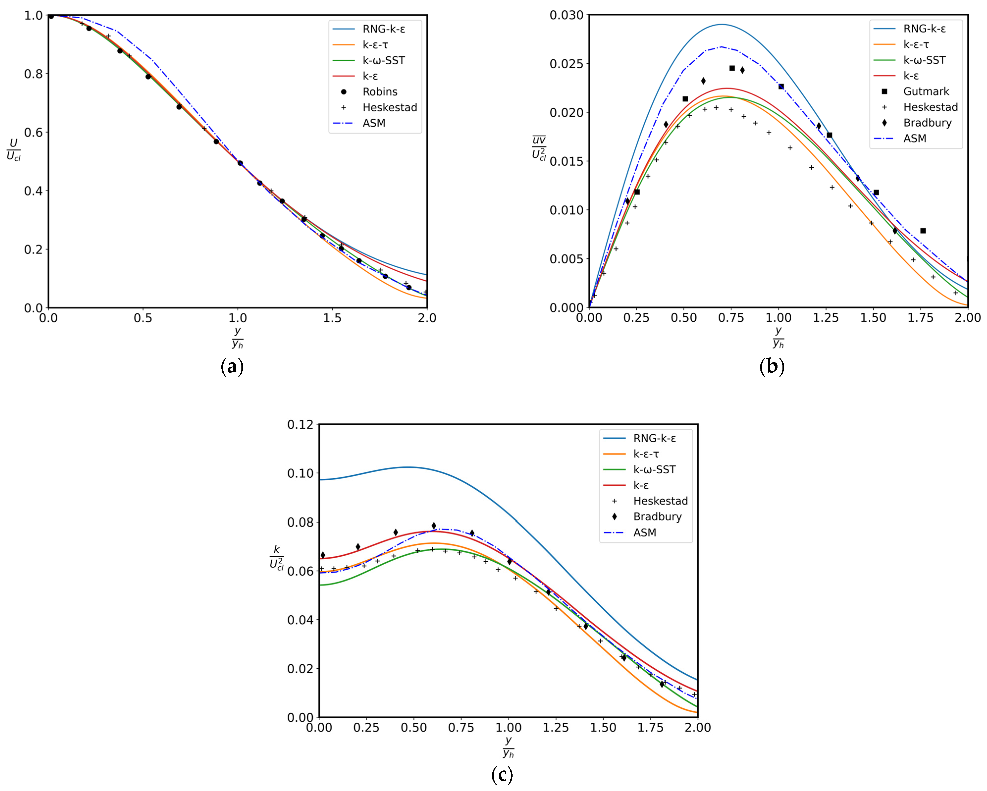
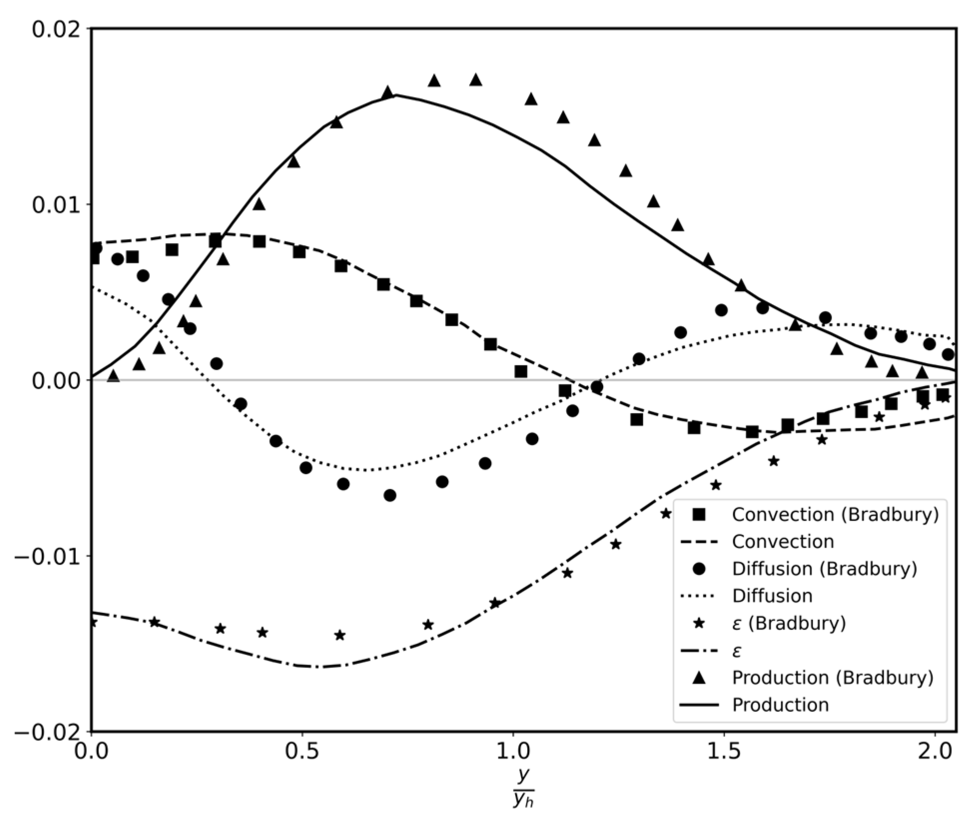
4.1. Plane Jet Results

Some of the early studies, by use of a hot wire anemometry, were performed by various researchers [35,36,37,38,39,40]. Simulation parameters such as boundary conditions (e.g., Re = 16,500) are similar to the work of Salerno [41]. According to the findings, jets that are released into stagnant environments eventually form self-similar states in which their time-averaged quantities may be expressed by only one length scale and one velocity. In other words, Reynolds stress and the mean velocity distribution must not depend on the streamwise coordinate “x”, as these scales are used to normalize them. A turbulent flow is said to be self-similar when some or all of its normalized statistical properties, such as half-width of the jet (spreading rate $=\partial y_h/\partial x$), become constant. Mean axial velocity distribution achieves self-similarity before the turbulence entities. However, there is no consensus on where this state is reached; it varies from x/d = 40 to 100. The calculated spreading rates exhibit a high degree of concordance with a value of $\partial y_h/\partial x$ of 0.109. TKE in the vicinity of the nozzle tip increases depending on its high production rate in regions characterized by a large velocity gradient. This high TKE produced in the high shear area diffuses towards the jet’s center and edge as it expands.

The turbulence quantity measurements are widely dispersed. The LDA measurement of Ramaprian and Chandrasekhara [42] gave the second lowest maximum shear stress level of ${\overline{uv}}_{max}/U_{cl}^2=$0.02, with the highest spreading rate of 0.112 (

Table 2. Comparison of experimental and model results for incompressible plane jet.

Investigator	Spreading Rate	${\overline{\mathit{u}\mathit{v}}}_{\mathit{m}\mathit{a}\mathit{x}}/{\mathit{U}}_{\mathit{c}\mathit{l}}^2$	Remarks
Bradbury [35]	0.109	0.024	HWA
Gutmark and Wygnanski [36]	0.11	0.024	HWA
Miller and Comings [37]	0.097	0.025	CTA
Van der Hegge Zijnen [39]	0.095	-	HWA
Heskestad [40]	0.11	0.020	HWA
Everitt and Robins [43]	0.09–0.11	0.019	CTA
Ramaprian and Chandrasekhara [42]	0.112	0.02	LDA
k–ε model	0.108	0.022
SST k–ω model	0.113	0.0215
RNG k–ε model	0.117	0.029
k–ε–τ model	0.109	0.0216

). For jets in stagnant environments, the self-similar form is regarded as universal and independent of the jet’s initial conditions. Consequently, a uniform TKE level ($k_j=1/2{\left(U_{0}I\right)}^2)$ and a flat velocity profile at the jet nozzle are selected as initial conditions, where I denotes turbulence intensity.

The computed mean velocity distribution for plane jets in the area of self-similarity is displayed in Figure 2 in the axial direction. It is assessed in comparison with the experimental results of Robins [38], and predictions of the other two-equation models considered in the current manuscript. Figure 2 presents a comparison of the shear stress “$\overline{uv}$” and TKE data from Gutmark and Wygnanski [36] and Bradbury [35], respectively. The modified k–ε–τ model provides better agreement for shear stress and complies with TKE patterns observed in both experimental findings documented in the scientific literature closer to the centre of the jet, and slightly underestimates shear stress towards the distance of 2y_h.

Table 2 displays the spreading-rates as well as the maximum shear stress levels achieved for the plane jet in comparison to different experimental results and values determined using various two-equation models. It is evident that the k–ε–τ model predicts spreading-rate far more accurately with a value of 0.109, and the maximum shear stress levels are also consistent with the revised model. This is not unexpected considering that the coefficients are modified in order to achieve optimal agreement among the turbulence quantities, spreading rate, and mean velocity.

The time scale $\tau$ can be normalized in two ways, either by ${\tau }^{\ast }=\tau U_{CL}/y_h$ or $z=\epsilon \tau /k$. The latter can also be expressed as the ratio of two different time scales and, it should be comparable to the reciprocal of $C_{\epsilon 2}$ of the standard k–ε model (1/1.92). Figure 3 shows time scales ${\tau }^{\ast }$ and z, respectively. ${\tau }^{\ast }$ is compared with values of $k/\epsilon$ (times $1/C_{\epsilon 2}$ of the k–ε model) predicted from both the k–ε and k–ε–τ models. Time scales of $k/\epsilon$ from both models go in parallel, the one predicted from the k–ε–τ model being 4% higher, across the jet. Time scale ${\tau }^{\ast }$ starts with the same value of $k/\epsilon$ of the k–ε model in the centre of the jet and slightly increases until about 1.5 y_h, yielding, at the maximum, a 7% higher value between 0.9 y_h to 1.4 y_h. Although the k–ε model suggests that its $C_{\epsilon 2}$ coefficient depends only on decay exponent, variation in “z” across the jet implies that the coefficient $C_{\epsilon 2}$ of the k–ε model would not be a true constant. The TKE budget, as found by the modified k–ε–τ model is compared in Figure 4 with the Bradbury’s energy balance, which is found to be more consistent than Gutmark’s, according to Rodi [44]. Agreement is again very good and consistent with the above findings.

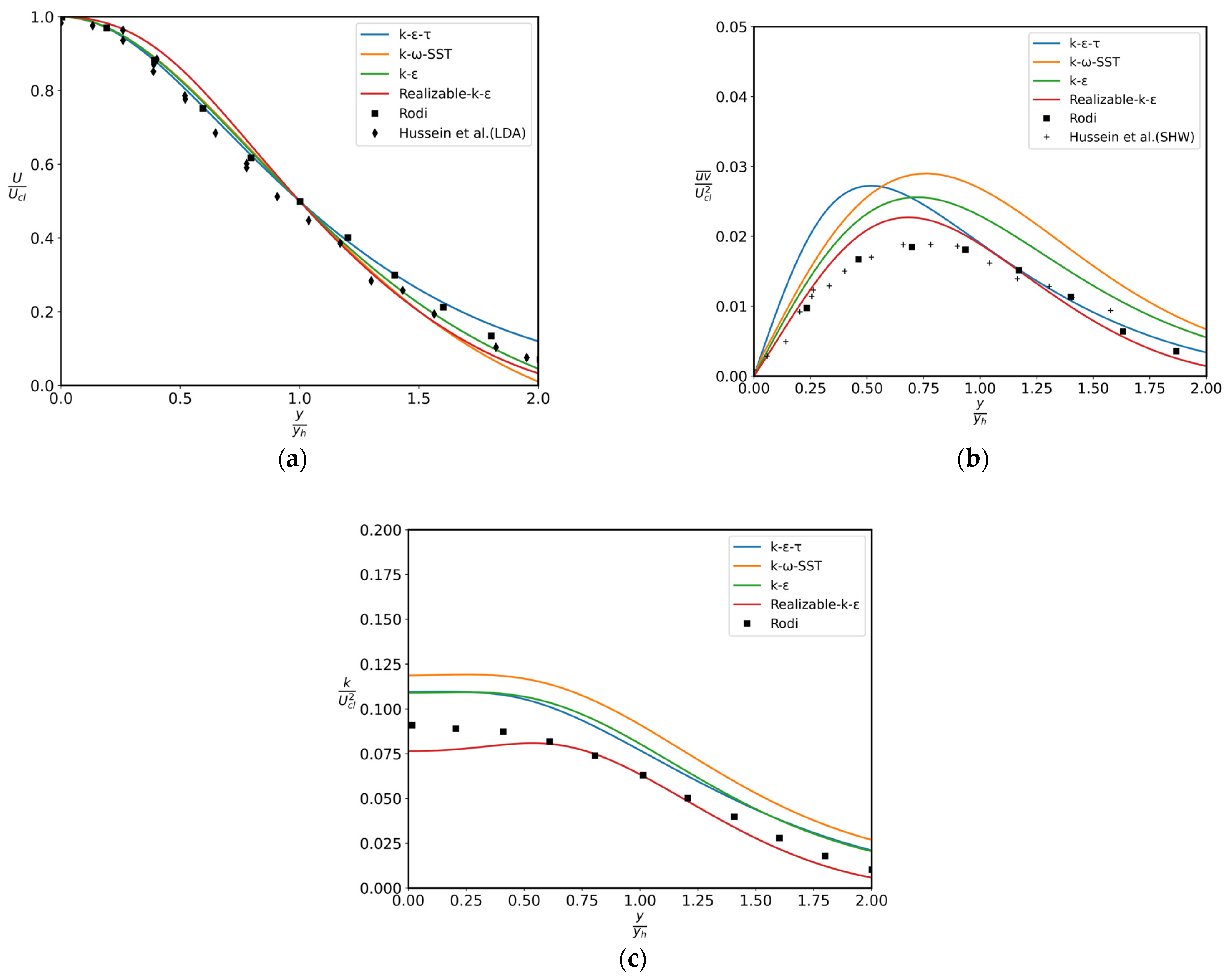
4.2. Round Jet Results

Table 3 gives a summary of experiments and simulation outcomes of the turbulence properties in the self-similar area. Compared to a plane jet, a round jet spreads slower, according to these observations, and takes between 50 and 70 diameters to achieve its self-similar form. Hussein and George [45] reported a peak value of about $\overline{uv}/U_{cl}^2=0.021$ at 70 x/d and gave a value of 0.094 for the spreading rate, although early research indicates a spreading rate of $d{y}_h/dx=0.086$. The work by Hussein et al. [46] contains the simulation parameters for round jet simulations, specifically Re = 95,500 and U_i = 56.2 m/s.

The traditional models consistently anticipate higher spreading rates for the axisymmetric case, also known as the “plane jet/round jet” anomaly, which was initially documented by Rodi and Spalding [47] in their analysis using the k–k_l model. However, the round jet spreading rates predicted by the SST k–ω and k–ε models are around 28% too high, while the k–ε–τ model (applying the identical model parameters to the plane jet) provides a considerably closer value of 0.089. A realizable k–ε model is close behind the k–ε–τ model in terms of spreading rates, with a value of 0.088.

Table 3. Comparison of experimental and model results for incompressible axisymmetric jet.

Investigator	Spreading Rate	${\overline{\mathit{u}\mathit{v}}}_{\mathit{m}\mathit{a}\mathit{x}}/{\mathit{U}}_{\mathit{c}\mathit{l}}^2$	Remarks
Hussein and George [45]	0.094	0.021	moving HW
Wygnanski and Fiedler [48]	0.086	0.0165	HWA
Rodi [49]	0.086	0.0186	HWA
Capp [50]	0.095	-	LDA
Panchapakesan and Lumley [51]	0.096	0.021	moving HW
Taulbee et al. [52]	0.094–0.102	0.021	LDA-HWA
$k–\epsilon$ model	0.120	0.025
$\mathrm{SST} k–\omega$ model	0.121	0.028
$\mathrm{Realizable} k–\epsilon$ model	0.088	0.023
$k–\epsilon –\tau$ model	0.089	0.027

Table 3. Comparison of experimental and model results for incompressible axisymmetric jet.

Investigator	Spreading Rate	${\overline{\mathit{u}\mathit{v}}}_{\mathit{m}\mathit{a}\mathit{x}}/{\mathit{U}}_{\mathit{c}\mathit{l}}^2$	Remarks
Hussein and George [45]	0.094	0.021	moving HW
Wygnanski and Fiedler [48]	0.086	0.0165	HWA
Rodi [49]	0.086	0.0186	HWA
Capp [50]	0.095	-	LDA
Panchapakesan and Lumley [51]	0.096	0.021	moving HW
Taulbee et al. [52]	0.094–0.102	0.021	LDA-HWA
$k–\epsilon$ model	0.120	0.025
$\mathrm{SST} k–\omega$ model	0.121	0.028
$\mathrm{Realizable} k–\epsilon$ model	0.088	0.023
$k–\epsilon –\tau$ model	0.089	0.027

The predicted mean axial velocity, shear stress, and TKE profiles for axisymmetric jets are compared to the work of Rodi [49] at the self-similar region in Figure 5. It is evident that consistency of the k–ε–τ model outputs are quite satisfactory. The maximum shear stress profiles are projected to be 22% higher by the k–ε model; that is compatible with the prediction of its spreading rate. The k–ε–τ model, after making a slight hump which is not consistent with experiments at about 0.5 y_h, levels with the data from the measurements of Rodi [49], and Hussein et al. [46]; thereafter, the agreement with it is quite good.

Interestingly, the aforementioned “plane jet/round jet” anomaly does not appear in the k–ε–τ model. Unlike the close error margin considering the plane jet, TKE profiles are overestimated by about 9% from the jet axis in the first quarter.

On the other hand, TKE predictions of the SST k–ω model are much higher than the rest of the models considered in the manuscript, in terms of both shear stress and TKE distributions.

Turbulence time scale ${\tau }^{\ast }$ level is consistently higher than the k–ε level in the k–ε–τ model, up to the outer edge of the jet, by about 5% at the jet centre and 12% at 1.4 y_h (Figure 6), but agrees with $k/\epsilon$ from the k–ε model. It can also be observed in the same figure that the z-level is increased slightly (7–8%) compared to plane jet (Figure 3). This could be due to an increased energy dissipation rate predicted in the round jet as can be seen in the energy budget in Figure 7. It can also be seen that the convection and production terms in the energy budget are predicted reasonably well compared with the measurements. The change in sign in the diffusion term, close to the centre of the jet, is consistent with the predictions of TKE. However, this is not supported by the experiments as seen in Figure 5 and Figure 7.

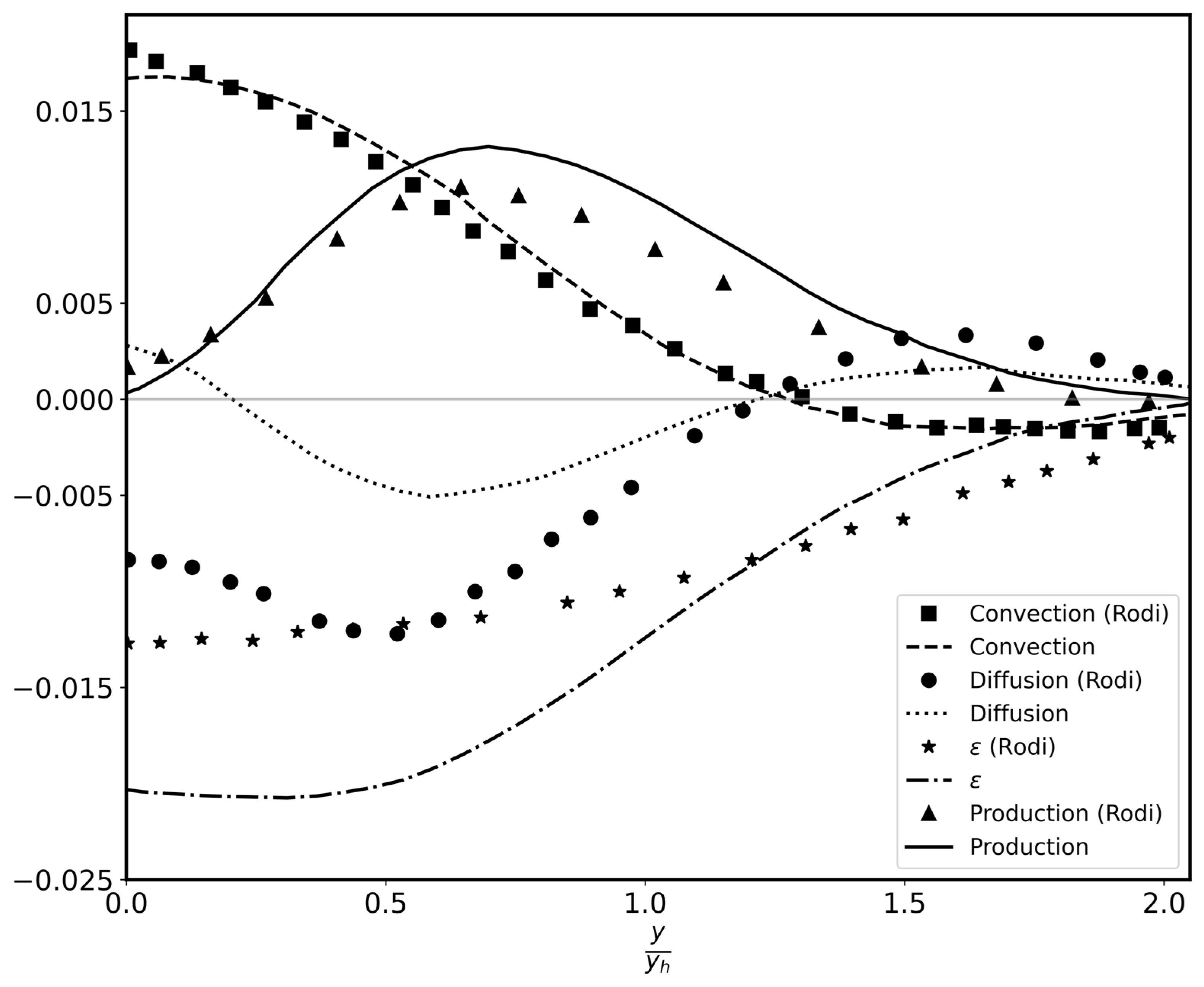
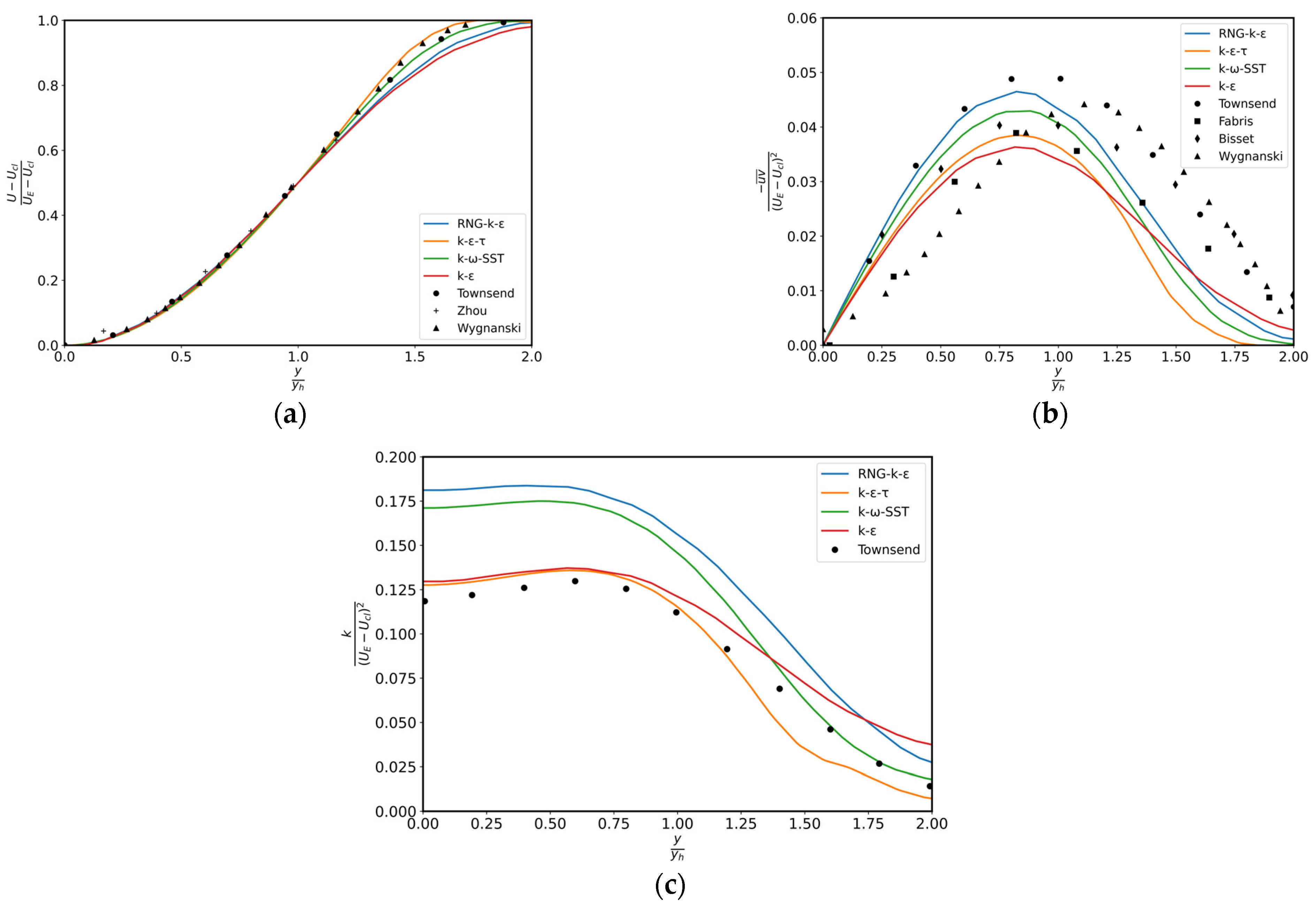
4.3. Plane Far Wake Results

It is possible to define a normalized spreading parameter for the wake as $S_w=\left(U_E/U_o\right)d{y}_h/dx$, where U_E is the outer stream velocity and U_o is the velocity deficit at the centerline of the wake [53,54]. The simulation parameters for plane far wake simulations are specified in the paper by Zhou et al. [54] as Re = 2800 and U_i = 6.7 m/s. Simulation results proved that the measurements of Wygnanski et al. [55] seemed to be the most reliable. They state that the Reynolds number calculated by using the cylinder diameter is equal to 1360 and that the similarity zone begins at x/D > 400 in the wake of the cylinder that has a certain diameter (D = 6.35 mm) [54]. Their similarity research suggests that the parameter for spreading must have a specific value, irrespective of the wake generator type. Furthermore, Louchez et al. [56] asserted that the plane wake reaches a universal, self-sustaining form that is independent of the initial body when it is sufficiently far downstream, depending on the self-preserving properties demonstrated by second order moments. However, measurements of Wygnanski et al. [55] suggested that the developing behavior and asymptotic structure of plane wake can be impacted by the form of the wake generator, and this was one of the causes of the disagreement observed by different workers.

It is particularly challenging to estimate both weak and strong shear flows using a pair of coefficients, particularly when employing eddy-viscosity models. The phenomenon known as “weak–strong shear flow” is thought to be induced by the dissipation rate equation in its simulated form.

Table 4. Comparison of experimental and model results for plane far wake.

Investigator	Spreading Parameter	$-{\overline{\mathit{u}\mathit{v}}}_{\mathit{m}\mathit{a}\mathit{x}}/{\mathit{U}}_{\mathit{c}\mathit{l}}^2$
Everitt and Robins [43]	0.096	0.037
Ermshaus (from Ramaprian and Chandrasekhara [42])	0.089	-
Wygnanski et al. [55]	0.082	0.048
Townsend [57]	0.098	0.051
Sreenivasan and Narasimha [58]	0.092	-
k–ε model	0.077	0.036
$\mathrm{SST} k–\omega$ model	0.079	0.042
$\mathrm{RNG} k–\epsilon$ model	0.099	0.046
k–ε–τ model	0.081	0.039

presents a compilation of experimental and projected values for the wake spreading parameters in the aftermath of the wake generator, as determined by the typical two-equation models and k–ε–τ model. Regarding the experiments of Wygnanski et al. [55], the modified k–ε–τ model underestimates this spread parameter by less than 2%, suggesting a considerably better result compared to the significant underestimation by the k–ε and SST k–ω models.

As can be seen in Figure 8, the mean axial velocity profile for the far wake is well predicted, and the result obtained is very similar to that of other models. Despite a 23% lower estimation of maximum shear stress level compared to experimental values [55], the modified k–ε–τ model yielded a better value than the k–ε model, which underestimated it by 33%. This finding aligns with the comparative evaluation of the models’ spreading parameter performance. Moreover, TKE profiles are predicted to be within 3% deviation close to the centre of the wake, up to the point of 1.2 y_h. Conversely, throughout the interval of 0–1.2 y_h, shear stress profiles are underestimated by approximately 15–30 percent, yielding a reduced level of concurrence in comparison to the other models considered in this research. When compared to experimental behavior, both turbulence energy profiles and shear stress appear to cease instantly near the outer edge.

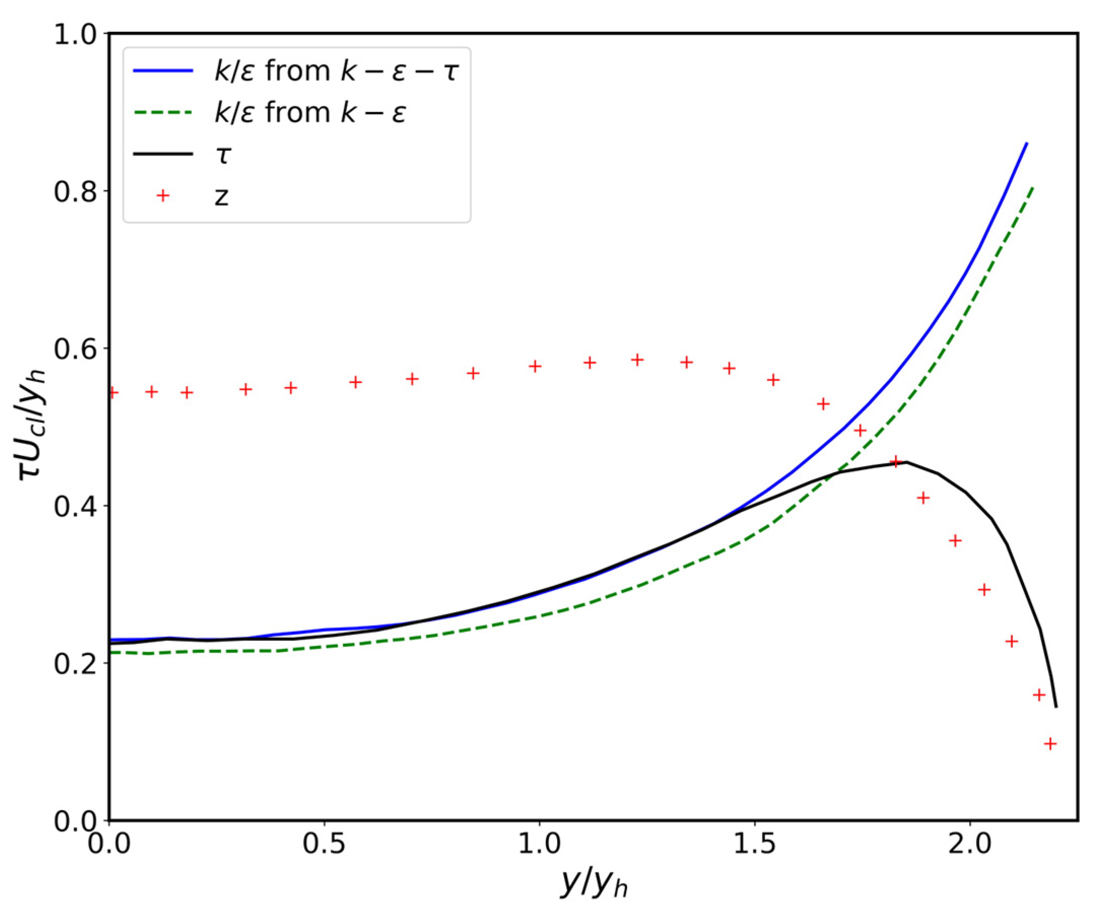
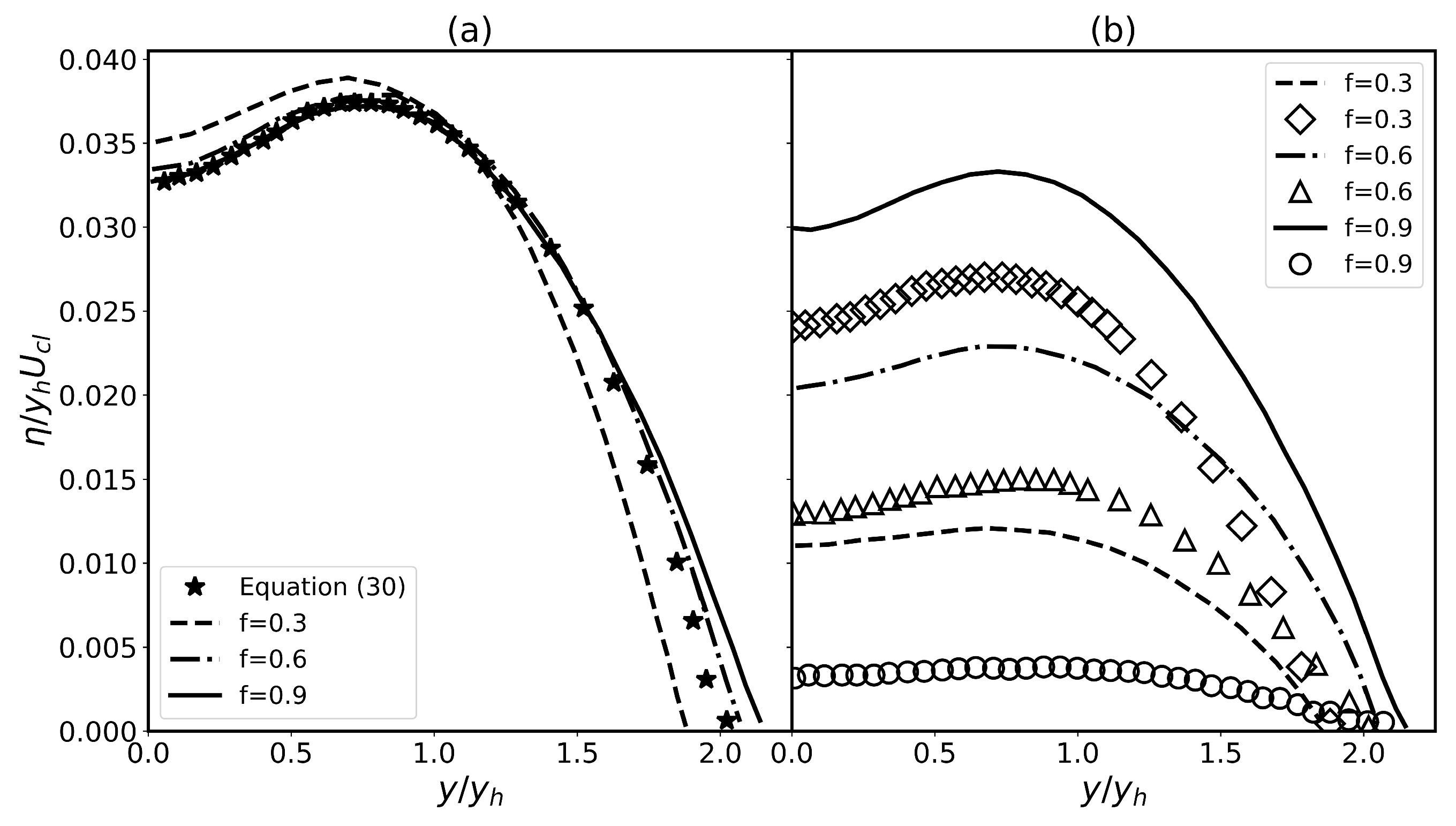
4.4. Turbulence Viscosity Relation

Since there are now two distinct time scales, there are two ways to quantify eddy viscosity: ${\mu }_t=C_{\mu }\rho k^2/\epsilon$ or ${\mu }_t=C_{\mu }\rho z_0^{-1}k\tau$, or more generally:

$${\mu }_t=C_{\mu }\rho \frac{k^2}{\epsilon }\left[f+\frac{z}{z_0}\left(1-f\right)\right]$$

(29)

where the weighting factor, f, can be chosen to give optimum agreement. Alternatively, partial replacement of time scale $k/\epsilon$ with $\tau /z_1$ yields another expression for turbulent viscosity:

$${\mu }_t=C_{\mu }\rho z_0^{-1/2}{k}^{3/2}{\left(\frac{\tau }{\epsilon }\right)}^{1/2}$$

(30)

which can also be interpreted as the geometric average of two length scales: $k^{3/2}/\epsilon$ and $k^{1/2}\tau$.

In Figure 9a, the normalized turbulence viscosities and, in Figure 9b, two of its components arising from the length scales “$k^{3/2}/\epsilon$” and “$k^{1/2}\tau$” (symbols in the figure), according to Equation (29), are presented for f = 0.9, f = 0.6, and f = 0.3. Inclusion of the time scale $\tau$ into the definition of turbulence viscosity as described in Equation (29) introduces a more abrupt variation in dependent variables towards the edge of the jet, as seen in Figure 9a for normalized ${\upsilon }_t$, and a slight increase in the spreading rate from 0.111 for f = 0.9 to 0.114 for f = 0.3, getting less stable for the latter. In Figure 9a, the turbulence viscosity distribution calculated from Equation (30) is also presented. However, this form also produces an abrupt change similar to f = 0.5 towards the edge and similar to f = 0.9 in the core region of the jet; nevertheless, it yields a spreading rate of 0.11 for plane jets.

5. Conclusions

In this study, a novel three-equation turbulence model was developed based on the limitations of the WFC model for predicting the behavior of shear flows, and its performance was then presented for plane and axisymmetric jets, and plane asymptotic wake.

The findings indicate that the k–ε–τ model outperforms the k–ε model by a significant margin. The first benefit is that the “plane jet/round jet” anomaly is better resolved by avoiding additional difficulties of second moment closures. The second benefit is that the flow behavior is better predicted than with the two-equation models in the wake, which is characterized by its weak shear form. Furthermore, it was discovered that:

• Consistent with the measurements, the three-equation model (utilizing identical parameters across all three cases) estimates a spread rate of 0.109 for the plane jet;
• The model estimates the round jet spreading rate of 0.089, which is over 23% better than the k–ε and SST k–ω models and consistent with the experimental data;
• The parameter for the spreading of the plane wake is estimated to be 0.081, which is approximately 6% more accurate than the k–ε model and 4% more accurate than the SST k–ω model;
• Time scales $\tau$ and $k/\epsilon$ behave quite similar to each other in most parts of the jet, as expected (in non-equilibrium situations, as in the compression stroke of an IC engine, these two will differ considerably);
• For the turbulence viscosity, several options, such as the geometric and arithmetic averages with a weighting factor, were investigated and shown to have no significant advantage over the traditional one for the types of flows tested.

References

1. Argyropoulos, C.D.; Markatos, N.C. Recent Advances on the Numerical Modelling of Turbulent Flows. Appl. Math. Model 2015, 39, 693–732. [Google Scholar] [CrossRef]
2. Klein, T.S.; Craft, T.J.; Iacovides, H. The Development and Application of Two-Time-Scale Turbulence Models for Non-Equilibrium Flows. Int. J. Heat Fluid Flow 2018, 71, 334–352. [Google Scholar] [CrossRef]
3. Klein, T.S.; Craft, T.J.; Iacovides, H. Assessment of the Performance of Different Classes of Turbulence Models in a Wide Range of Non-Equilibrium Flows. Int. J. Heat Fluid Flow 2015, 51, 229–256. [Google Scholar] [CrossRef]
4. Nie, X.; Chen, Z.; Zhu, Z. Assessment of Low-Reynolds Number k-ε Models in Prediction of a Transitional Flow with Coanda Effect. Appl. Sci. 2023, 13, 1783. [Google Scholar] [CrossRef]
5. Wu, C.-T.; Ferziger, J.-H.; Chapman, D.-R. Simulation and Modeling of Homogeneous, Compressed Turbulence. In Proceedings of the 5th Symposium on Turbulent Shear Flows, Ithaca, NY, USA, 7–9 August 1985; pp. 17.13–17.19. [Google Scholar]
6. Le Penven, L.; Serre, G. A Generalized κ-ε Model for Compressed Turbulence. In Proceedings of the Eurotherm 15, Toulouse, France, 4–6 December 1991. [Google Scholar]
7. Hamlington, P.E.; Ihme, M. Modeling of Non-Equilibrium Homogeneous Turbulence in Rapidly Compressed Flows. Flow Turbul. Combust. 2014, 93, 93–124. [Google Scholar] [CrossRef]
8. Kim, S.W.; Chen, C.P. A Multiple-Time-Scale Turbulence Model Based on Variable Partitioning of the Turbulent Kinetic Energy Spectrum. Numer. Heat Transf. Part B Fundam. 1990, 16, 193–211. [Google Scholar] [CrossRef]
9. Hanjalic, K.; Launder, B.; Schiestel, R. Multiple-Time-Scale Concepts in Turbulent Transport Modeling. In Proceedings of the Turbulent Shear Flows 2, London, UK, 4 July 1980; Springer: Berlin/Heidelberg, Germany, 1980; pp. 36–49. [Google Scholar]
10. Chitta, V.; Dhakal, T.P.; Walters, D.K. Development and Application of a New Four-Equation Eddy-Viscosity Model for Flows With Transition, Curvature and Rotation Effects. In Proceedings of the Fluids Engineering Division Summer Meeting, Incline Village, NV, USA, 7 July 2013; ASME: New York, NY, USA, 2013; pp. 1–10. [Google Scholar]
11. Grunloh, T.P. Four Equation K-Omega Based Turbulence Model with Algebraic Flux for Supercritical Flows. Ann. Nucl. Energy 2019, 123, 210–221. [Google Scholar] [CrossRef]
12. Zeierman, S.; Wolfshtein, M. Turbulent Time Scale for Turbulent-Flow Calculations. AIAA J. 1986, 24, 1606–1610. [Google Scholar] [CrossRef]
13. Catris, S.; Aupoix, B. Towards a Calibration of the Length-Scale Equation. Int. J. Heat Fluid Flow 2000, 21, 606–613. [Google Scholar] [CrossRef]
14. Chen, C.J.; Singh, K. Development of a Two-Scale Turbulence Model and Prediction of Buoyant Shear Flows. In Proceedings of the AIAA/ASME Thermophsics and Heat Transfer Conference, Seattle, WA, USA, 16–18 June 1990; HTD Publication: Washington, DC, USA, 1990. [Google Scholar]
15. Jaw, S.Y.; Hwang, R.R. A Two-Scale Low-Reynolds Number Turbulence Model. Int. J. Numer. Methods Fluids 2000, 33, 695–710. [Google Scholar] [CrossRef]
16. Morgan, B.E.; Schilling, O.; Hartland, T.A. Two-Length-Scale Turbulence Model for Self-Similar Buoyancy-, Shock-, and Shear-Driven Mixing. Phys. Rev. E 2018, 97, 013104. [Google Scholar] [CrossRef]
17. Lumley, J.L. Some Comments on Turbulence. Phys. Fluids A 1992, 4, 203–211. [Google Scholar] [CrossRef]
18. Goldberg, U.C. Exploring a Three-Equation r-k-ϵ Turbulence Model. J. Fluids Eng. Trans. ASME 1996, 118, 795–799. [Google Scholar] [CrossRef]
19. Baldwin, B.S.; Barth, T.J. A One-Equation Turbulence Transport Model for High Reynolds Number Wall-Bounded Flow; Ames Research Center: Moffett Field, CA, USA, 1990. [Google Scholar]
20. Cotton, M.A.; Ismael, J.O. A Strain Parameter Turbulence Model and Its Application to Homogeneous and Thin Shear Flows. Int. J. Heat Fluid Flow 1998, 19, 326–337. [Google Scholar] [CrossRef]
21. Billard, F.; Laurence, D. A Robust K-ε-V2/k Elliptic Blending Turbulence Model Applied to near-Wall, Separated and Buoyant Flows. Int. J. Heat Fluid Flow 2012, 33, 45–58. [Google Scholar] [CrossRef]
22. Wilcox, D.C. Multiscale Model for Turbulent Flows. AIAA J. 1988, 26, 1311–1320. [Google Scholar] [CrossRef]
23. Duranti, S.; Pittaluga, F. Navier-Stokes Prediction of Internal Flows with a Three-Equation Turbulence Model. AIAA J. 2000, 38, 1098–1100. [Google Scholar] [CrossRef]
24. Chen, C.P.; Guo, K. A Non-Isotropic Multiple-Scale Turbulence Model. Appl. Math. Mech. 1991, 12, 981–991. [Google Scholar] [CrossRef]
25. Nagano, Y.; Hattori, H. Improvement of an LRN Two-Equation Turbulence Model Reflecting Multi-Time Scales. Int. J. Heat Fluid Flow 2015, 51, 221–228. [Google Scholar] [CrossRef]
26. Ertesvag, I.S.; Byggstoyl, S.; Magnussen, B.F. An “Eddy-Dissipation” Reynolds-Stress Turbulence Model Closed by an Equation Related to the Turbulent Transport Timescale. In Proceedings of the 7th Symposium on Turbulent Shear Flows, Stanford, CA, USA, 23 August 1989; PSU: State College, PA, USA, 1989; Volume 2, pp. 17.3.1–17.3.6. [Google Scholar]
27. Ma, T.; Lucas, D.; Jakirlić, S.; Fröhlich, J. Progress in the Second-Moment Closure for Bubbly Flow Based on Direct Numerical Simulation Data. J. Fluid Mech. 2020, 883, A9. [Google Scholar] [CrossRef]
28. Lopez, M.; Walters, D.K. Prediction of Transitional and Fully Turbulent Flow Using an Alternative to the Laminar Kinetic Energy Approach. J. Turbul. 2016, 17, 253–273. [Google Scholar] [CrossRef]
29. Launder, B.E.; Spalding, D.B. The Numerical Computation of Turbulent Flows. Comput. Methods Appl. Mech. Eng. 1974, 3, 269–289. [Google Scholar] [CrossRef]
30. Yakhot, V.; Orszag, S.A.; Thangam, S.; Gatski, T.B.; Speziale, C.G. Development of Turbulence Models for Shear Flows by a Double Expansion Technique. Phys. Fluids A 1992, 4, 1510–1520. [Google Scholar] [CrossRef]
31. Menter, F.R. Two-Equation Eddy-Viscosity Turbulence Models for Engineering Applications. AIAA J. 1994, 32, 1598–1605. [Google Scholar] [CrossRef]
32. Shih, T.-H.; Liou, W.W.; Shabbir, A.; Yang, Z.; Zhu, J. A New K-ϵ Eddy Viscosity Model for High Reynolds Number Turbulent Flows. Comput. Fluids 1995, 24, 227–238. [Google Scholar] [CrossRef]
33. Moukalled, F.; Mangani, L.; Darwish, M. The Finite Volume Method in Computational Fluid Dynamics; Fluid Mechanics and Its Applications; Springer International Publishing: Cham, Switzerland, 2016; Volume 113, ISBN 978-3-319-16873-9. [Google Scholar]
34. Bailly, C.; Comte-Bellot, G. Turbulence; Experimental Fluid Mechanics; Springer International Publishing: Cham, Switzerland, 2015; ISBN 978-3-319-16159-4. [Google Scholar]
35. Bradbury, L.J.S. The Structure of a Self-Preserving Turbulent Plane Jet. J. Fluid Mech. 1965, 23, 31–64. [Google Scholar] [CrossRef]
36. Gutmark, E.; Wygnanski, I. The Planar Turbulent Jet. J. Fluid Mech. 1976, 73, 465–495. [Google Scholar] [CrossRef]
37. Miller, D.R.; Comings, E.W. Static Pressure Distribution in the Free Turbulent Jet. J. Fluid Mech. 1957, 3, 985. [Google Scholar] [CrossRef]
38. Robins, A. The Structure and Development of a Plane Turbulent Free Jet. Ph.D. Thesis, University of London, London, UK, 1973. [Google Scholar]
39. Van der Hegge Zijnen, B.G. Measurements of the Velocity Distribution in a Plane Turbulent Jet of Air. Appl. Sci. Res. Sect. A 1958, 7, 256–276. [Google Scholar] [CrossRef]
40. Heskestad, G. Hot-Wire Measurements in a Plane Turbulent Jet. J. Appl. Mech. Trans. ASME 1964, 32, 721–734. [Google Scholar] [CrossRef]
41. Salerno, S. RANS and LES Simulations of a Turbulent Plane Jet. Master’s Thesis, Politecnico di Milano, Milan, Italy, 2018. [Google Scholar]
42. Ramaprian, B.R.; Chandrasekhara, M.S. LDA Measurements in Plane Turbulent Jets. J. Fluids Eng. Trans. ASME 1985, 107, 264–271. [Google Scholar] [CrossRef]
43. Everitt, K.W.; Robins, A.G. The Development and Structure of Turbulent Plane Jets. J. Fluid Mech. 1978, 88, 563–583. [Google Scholar] [CrossRef]
44. Rodi, W. A Review of Experimental Data of Uniform Density Free Turbulent Boundary Layers; Launder, B.E., Ed.; Academic Press: Cambridge, MA, USA, 1975. [Google Scholar]
45. Hussein, H.J.; George, W.K. Measurement of Small Scale Turbulence in an Axisymmetric Jet Using Moving Hot-Wires. In Proceedings of the 7th Symposium on Turbulent Shear Flows, Stanford, CA, USA, 23 August 1989; PSU: State College, PA, USA, 1989; Volume 2, pp. 30.2.1–30.2.6. [Google Scholar]
46. Hussein, H.J.; Capp, S.P.; George, W.K. Velocity Measurements in a High-Reynolds-Number, Momentum-Conserving, Axisymmetric, Turbulent Jet. J. Fluid Mech. 1994, 258, 31–75. [Google Scholar] [CrossRef]
47. Rodi, W.; Spalding, D.B. A Two-Parameter Model of Turbulence, and Its Application to Free Jets. Wärme Stoffübertrag. 1970, 3, 85–95. [Google Scholar] [CrossRef]
48. Wygnanski, I.; Fiedler, H. Some Measurements in the Self-Preserving Jet. J. Fluid Mech. 1969, 38, 577–612. [Google Scholar] [CrossRef]
49. Rodi, W. The Prediction of Free Turbulent Boundary Layers by Use of a Two-Equation Model of Turbulence. Ph.D. Thesis, University of London, London, UK, 1972. [Google Scholar]
50. Capp, S.P. Experimental Investigation of the Turbulent Axisymmetric Jet. Ph.D. Thesis, State University of New York, New York, NY, USA, 1983. [Google Scholar]
51. Panchapakesan, N.; Lumley, J.L. Turbulence measurements in axisymmetric jets of air and helium. Part 1. Air jet. J. Fluid Mech. 1993, 246, 197–223. [Google Scholar] [CrossRef]
52. Taulbee, D.B.; Hussein, H.; Capp, S. Round Jet—Experiment and Inferences on Turbulence Modeling. In Proceedings of the 6th Symposium on Turbulent Shear Flows, Toulouse, France, 7–9 September 1987; pp. 10-5-1–10-5-6. [Google Scholar]
53. Newman, B.G. Turbulent Jets and Wakes in a Pressure Gradient; DDC: Virginia Beach, VA, USA, 1967. [Google Scholar]
54. Zhou, Y.; Antonia, R.A.; Tsang, W.K. The Effect of Reynolds Number on a Turbulent Far-Wake. Exp. Fluids 1998, 25, 118–125. [Google Scholar] [CrossRef]
55. Wygnanski, I.; Champagne, F.; Marasli, B. On the Large-Scale Structures in Two-Dimensional, Small-Deficit, Turbulent Wakes. J. Fluid Mech. 1986, 168, 31. [Google Scholar] [CrossRef]
56. Louchez, P.R.; Kawall, J.G.; Keffer, J.F. Investigation of the Detailed Spread Characteristics of Plane Turbulent Wakes. In Proceedings of the Fifth Symposium on Turbulent Shear Flows, New York, NY, USA, 9 August 1985; Cornell University: Ithaca, NY, USA; pp. 98–109. [Google Scholar]
57. Townsend, A.A. The Fully Developed Turbulent Wake of a Circular Cylinder. Aust. J. Sci. Res. Ser. A Phys. Sci. 1949, 2, 451–468. [Google Scholar]
58. Sreenivasan, K.R.; Narasimha, R. Equilibrium Parameters for Two-Dimensional Turbulent Wakes. J. Fluids Eng. Trans. ASME 1982, 104, 167–169. [Google Scholar] [CrossRef]
59. Fabris, G. Conditional sampling study of the turbulent wake of a cylinder. Part 1. J. Fluid Mech. 1979, 94, 673–709. [Google Scholar] [CrossRef]
60. Bisset, D.K.; Antonia, R.A.; Browne, L.W.B. Spatial organization of large structures in the turbulent far wake of a cylinder. J. Fluid Mech. 1990, 218, 439–461. [Google Scholar] [CrossRef]
Figure 1. Return to equilibrium of z.
Applsci 14 01133 g001
Figure 2. Prediction of (a) mean axial velocity, (b) shear stress, and (c) TKE profiles for plane jets [35,36,38,40].
Applsci 14 01133 g002
Figure 3. Estimation of z-profiles and the turbulence time scale in plane jet.
Applsci 14 01133 g003
Figure 4. Plane jet energy budget.
Applsci 14 01133 g004
Figure 5. Prediction of (a) mean axial velocity, (b) shear stress, and (c) TKE profiles for round jets [45,46,49].
Applsci 14 01133 g005
Figure 6. Estimation of z-profiles and turbulence time scale in round jet.
Applsci 14 01133 g006
Figure 7. Round jet energy budget [49].
Applsci 14 01133 g007
Figure 8. (a) Mean axial velocity, (b) u v ¯ shear stress, and (c) TKE profiles for plane far wake [54,55,57,59,60].
Applsci 14 01133 g008
Figure 9. (a) Normalized turbulence viscosities across the plane jet for a range of “f”. (b) Turbulence viscosity components for a range of “f” that originates from two distinct length scales.
Applsci 14 01133 g009