Deepwater 3D Measurements with a Novel Sensor System

Featured Application

The potential application of the introduced sensor system can enable the simultaneous mapping of the seafloor and the capturing of high-precision 3D data of underwater industrial structures for inspection.

Abstract

A novel 3D sensor system for underwater application is presented, primarily designed to carry out inspections on industrial facilities such as piping systems, offshore wind farm foundations, anchor chains, and other structures at deep depths of up to 1000 m. The 3D sensor system enables high-resolution 3D capture at a measuring volume of approximately 1 m³, as well as the simultaneous capture of color data using active stereo scanning with structured lighting, producing highly accurate and detailed 3D images for close-range inspection. Furthermore, the system uses visual inertial odometry to map the seafloor and create a rough 3D overall model of the environment via Simultaneous Localization and Mapping (SLAM). For this reason, the system is also suitable for geological, biological, or archaeological applications in underwater areas. This article describes the overall system and data processing, as well as initial results regarding the measurement accuracy and applicability from tests of the sensor system in a water basin and offshore with a Remotely Operating Vehicle (ROV) in the Baltic Sea.

1. Introduction

Robots and sensors are increasingly used in various underwater applications, such as inspection, biological research and documentation, climate and weather observations, the documentation and monitoring of coastal areas and archaeological sites, shipwreck exploration and documentation, and even the salvage of weapons.

Whereas robots undertake the task of divers, facilitate assembly processes, and decrease the risk of humans, sensors help to better understand the underwater environment. Underwater robots and divers can complement each other perfectly for certain tasks. Accordingly, special underwater sensor technology should be designed for both diver use and ROV connections, e.g., for deep sea applications.

Different kinds of sensors, such as optical, acoustic, biological, chemical, electromagnetic, and multimodal sensors, are increasingly used in underwater applications.

Underwater 3D metrology is one of the most dynamically developing disciplines of underwater applications for the inspection tasks of industrial structures such as offshore wind foundations, pipeline systems for oil and gas transport, and cable or anchor chain inspections. For these purposes, new 3D measurement systems with improved features and easier handling are currently being developed.

Various non-contact methods are available for 3D reconstruction underwater, e.g., techniques with sonar systems [1,2,3], laser scanning [4], time-of-flight measurements (ToFs) [5,6], and photogrammetry [7,8,9,10].

Optical time-of-flight (ToF) sensors, which are based on the temporal evaluation of light pulses, provide similar accuracy to acoustic systems for 3D underwater measurements. These systems, based on LiDAR technology, are available, for example, from the company 3D at Depth [5]. Mariani et al. [6] present a new ToF-based measurement system called UTOFIA.

Laser scanner systems are suitable for obtaining 3D data underwater and addressing the challenges posed by long distances and cloudy water [11,12,13]. These measurements can also be carried out in motion and offer a high level of robustness. As a rule, laser systems are based on the capture of individual lines, which must be merged into a 3D scan.

Visual odometry is used to estimate vehicle navigation and motion data [14]. Generated motion data are used, for example, for the 3D mapping of the route traveled, but has a much lower accuracy than measurement data obtained from photogrammetry.

Underwater photogrammetry has been used for decades for the highly accurate reconstruction of objects such as shipwrecks [7,8]. However, a lot of preparation work is required to achieve a high level of measurement accuracy. This concerns the placement of markers and textured objects or the support of structured lighting. Furthermore, static measurements, in which neither the measuring system nor the measurement object moves at all or only very slowly, require a lot of logistical effort. A large amount of time must be planned for the acquisition of a small measurement volume. Kwon [15], Telem and Filin [16], Sedlazeck and Koch [17], and others [18,19] present photogrammetric 3D measurement systems for underwater use. Beall [20] took a different approach, using video streams from a stereo camera. This involved merging successive 3D scans to reconstruct large underwater structures with low accuracy. Skinner [21] uses a plenoptic camera for underwater 3D measurements.

Underwater 3D measurement systems with structured lighting are currently experiencing increasing development and testing but are not yet used commercially. The main reason for this is the short range and the comparatively small measuring volume compared to laser-based systems. Systems with structured lighting have been described in recent years by, for example, Bruno et al. [22] and Bianco et al. [23].

Structured light-supported systems have significant potential in terms of the high measurement accuracy of this reconstruction technique.

The absolute accuracy of photogrammetric 3D measuring systems for applications in the air can be up to 1:10,000 (see [24]), i.e., for measured variables such as lengths of 1 m, the absolute error can be less than 0.1 mm. In underwater applications, the absolute measurement accuracy is limited due to unfavorable environmental conditions such as beam refraction, water turbidity, suspended particles in the water, etc., with up to 1:1000 but are still high compared to ToF and sonar systems. When using structured illumination, the measurement accuracy can be increased even further for objects with a limited natural surface structure compared to passive photogrammetry.

However, for the illumination of distant objects with a large field of view, the illumination output of the sample projectors is typically too weak. Additionally, short scanning times, fast data processing, and the creation of 3D surface models in real-time are required. Hence, advanced camera technology and powerful computing equipment to process large amounts of data are necessary. It is expected that new hardware developments will be able to meet these requirements soon.

The quality of a 3D measurement system depends heavily on its ability to compensate for the influence of the sensor or the measurement of object movements on captured 3D data. This is one of the most demanding tasks in 3D stereo scanning systems based on structured lighting because of the long exposure times required for a single scan. As a rule, ten subsequent images are required to realize a point of correspondence.

The distance traveled by a moving sensor in the time required to capture ten images results in the displacement (or blurring) of the projected pattern observed in a particular pixel. Motion correction can reduce or correct the resulting image distortion.

Various methods are available for movement compensation. A new method for pattern projection-based 3D scanner systems involving a projection unit in the 3D point calculation is presented by Lam et al. [25]. Furukawa et al. [26] describe the use of motion blur for motion compensation.

Recent applications have targeted the use of low-cost components in 3D reconstruction in coastal shallow waters using video streams from an action sports camera [27]. Structure-from-motion technology (SfM) was used to create an overall 3D model from the measurements [28].

With our novel underwater 3D sensor system, we attempted to obtain the precise, continuous 3D capturing and modeling of underwater structures at medium-range measurement distances and speeds of up to 1 m/s while processing it into a complete 3D model of the observed scene with a high level of detail.

The novelty of the presented system compared to commercially available underwater 3D measurement systems is the combination of the SLAM technology based on visual odometry (vSLAM) with highly precise, detailed 3D measurements of objects and the generation of dense, high-resolution 3D models, including color capture.

This work describes a novel 3D sensor system, which is suitable for underwater inspection tasks at sea depths of up to 1000 m by connecting it to a work-class Remotely Operating Vehicle (ROV). First, the hardware of the system is described, and the measurement properties are presented. Experimental measurement examples for practical applications are given, as well as measurements for the metrological characterization of the sensor system.

2. Materials and Methods

2.1. Underwater 3D Sensor System

2.1.1. Sensor Hardware

The new sensor system (called UWS) was developed as part of a publicly funded joint project in cooperation with project partners from industry and research. Two demonstrator variants (UWS1 and UWS2) of the same hardware configuration with different geometric designs were set up and used in the measurements. The sensor system consists of the following components:

• Two monochrome measurement cameras (type Baumer VLTX-28M.I with lenses SCHNEIDER KMP-IR CINEGON 12/1.4);
• A projection unit (in-house manufactured with lens SCHNEIDER STD XENON 17/0.95);
• A color camera (type Baumer VLTX-71M.I with lens SCHNEIDER KMP CINEGON 10/1.9);
• A Fiber Optic Gyro Inertial Measurement Unit (IMU, type KVH 1750 IMU);
• Two flashlights (using Cree CXB3590 LEDs);
• An electronic control box (in-house manufactured);
• Cylindrical underwater housing for individual components;
• Wiring for power supply and data transfer.

A schematic view of the sensor system is shown in Figure 1.

The components of the sensor system are integrated into four underwater housings. Two monochrome measurement cameras are installed as a stereo pair in the outer two housings. These are used in combination with a pattern projector installed in one of the central housings for 3D measurements. The projector generates aperiodic-sinusoidale fringe patterns for the 3D measurement and consists of an LED operating in the blue wavelength range with a high light output, a rotating glass mask, a motor, and a projection lens, which is the so-called GoBo-projection [29]. In addition, electrical drivers and control electronics are integrated into the same housing. Next to the underwater housing for the projector, there is another housing that contains the color camera and an inertial measurement unit (IMU) with a fiber optic gyroscope. The underwater housings are mounted together on a carbon fiber rod, which is decoupled from the support frame. There are also two LED flashlights on the outside of the sensor carrier. These are arranged such that they primarily illuminate the measurement object and do not illuminate particles in the close range of the camera to minimize backscatter. On the sensor carrier, there is a fifth underwater housing with the electronics of the power supply and network technology for data transmission.

All sensor data are transmitted via a network. For this purpose, a glass fiber from the tether of the diving robot is used during the measurement. The 3D calculation and evaluation of the data takes place outside the water on a PC workstation on the ship, which is connected directly to the sensor via a ten-gigabit fiber optic link. This means that there is no need to integrate powerful hardware for calculations in the underwater housing, thereby saving cost and weight. The 3D reconstruction and parts of the further processing take place online to enable the direct quality control of the recordings.

The difference between the UWS1 and UWS2 versions lies in the more compact arrangement of the components in the UWS2 sensor. This means that the image fields and the standard measuring distance change for identical cameras and lenses. Consequently, the UWS2 system results in a reduction in the standard measuring distance from 2.0 m to 1.3 m, a smaller field of view of 0.7 m × 0.6 m, and a brighter illumination of the scene. However, due to the necessary shorter distances to the measurement objects, the UWS2 system must be navigated more precisely by the ROV pilot to avoid collisions with the seabed or the measurement objects.

The monochrome measurement cameras are arranged in a typical stereo configuration [29] and are used to record images for the calculation of the detailed 3D data sets. They can be operated with a resolution of 2.8 MPix at a frame rate of 411 Hz. In the typical measurement mode, a 1 MPix resolution is used, with a frame rate of up to 900 Hz.

Three-dimensional image data are calculated by evaluating image sequencing pairs, one sequence from each camera, where each image sequence typically comprises ten images. The corresponding measurement principle is described in [29].

To support the determination of point correspondence in the two measurement cameras, the scene is illuminated with a structured stripe pattern by the projection unit. The GoBo method [29] is used for this, in which the stripe pattern is generated by projecting a rotating GoBo wheel. The main components of the projection unit are the lighting unit, rotary motor, GoBo wheel, projection lens, and the associated electronics. The lighting unit consists of a high-performance LED in the blue wavelength range. The projection lens is a typical industrial camera lens.

The color camera has 7 MPix and essentially fulfills two functions. Firstly, it serves to support the ROV pilot’s navigation when the ROV headlights are switched off. The ROV headlights cannot be switched on while the measurement is in progress, as they would disrupt the structured light pattern for the 3D measurement. The necessary lighting of the scene for the color camera recording is provided by the two flashlights, which are switched on and off alternately with the structured lighting. The second function of the color camera is the recording of video streams to create a 3D map of the scanned area of the seabed and the objects to be measured in the water. This is performed with the additional use of IMU data by means of visual odometry [14,30].

The inertial measurement unit (IMU) is used to register the sensor system’s own movement and to export these movement data to the control system of the UWS. Using this information, motion compensation for the 3D reconstruction can be performed online. With the help of IMU data and the color camera images, a trajectory of the sensor movement is generated afterward, which is also used for scaling the 3D data generated by the monocular video sequences using visual odometry.

The following features and performance parameters characterize the 3D measurement system UWS1. Distinguishing parameters of the second variant (UWS2) are listed in parentheses.

• Size (spatial dimensions): 1.25 m × 0.7 m × 0.5 m (0.9 m × 0.7 m × 0.5 m);
• Mass: 65 kg (approx.);
• Color camera frame rate: 25 Hz at 7 Mpix resolution;
• Measurement camera frame rate: up to 900 Hz at 1 MPix resolution;
• Three-dimensional frame rate: up to 50 Hz;
• Measurement distance 2.0 m ± 0.4 m (1.3 m ± 0.3 m);
• Field of view at a standard distance: 0.9 m × 0.8 m (0.7 m × 0.6 m);
• Maximum diving depth: 1000 m.

2.1.2. Software Architecture

In order to manage the control of all functions of the sensor system and data transfer, from the image recording to the monitoring of the final 3D model of the observed scene, a software concept was developed, as shown in the scheme of Figure 2, and implemented.

This concept was realized in such a way that certain data were available in real-time to support rough 3D reconstruction result monitoring with a time delay below 200 ms. This short latency time is necessary because incomplete 3D measurements must be prevented. If the operator identifies the need for a repeated measurement because of incomplete 3D data results, they can immediately navigate the ROV with the sensor system back to the relevant position.

2.1.3. Graphical User Interface

A key factor in the effective use of this sensor for measuring applications is the user interface developed as part of the project. This software provides visualization for the ROV pilot as well as the interface for the operator of the sensor system.

The software takes over the parameterization of the sensors to quickly adapt the exposure time and light sensitivity to the environmental conditions in the water. Furthermore, it helps to detect incorrect recordings in certain areas of the image and directly displays the 3D reconstruction result for quality control. In addition, the user interface allows the operator to control the data stream recording as well as trigger individual recordings, e.g., as part of the calibration process or 3D measurement. The ROV pilot shows the color image stream with a short latency in a separate software application. The color image can be adapted to the ambient conditions during the operation using various contrast improvement options.

To support navigation, the measuring distance is also displayed. The visualization of 3D data, which is more difficult to interpret than color images, is not necessary for the ROV pilot. To visualize the complete 3D model, a browser-based solution using Potrees [31] was developed. This includes user management, organization in scan projects, and the automated generation of point cloud previews.

Two examples of GUI are shown in Figure 3.

To enable remote access and 3D data observation without special 3D software tools, web technology was chosen. This means that anyone interested could observe and analyze data independently. In addition, it enabled data transmission via a cellular network or a satellite connection between the measurement location and an office location. This promoted parallel data analysis and could reduce the amount of personnel on the ship during the measurement process.

2.2. Data Recording

2.2.1. Generation of Measurement Data

The sensor system produces two kinds of three-dimensional measurement data. The first kind is a rough 3D data stream of the detected seabed environment below the realized path of the sensor system. This kind of data generation is also known as Simultaneous Localization and Mapping (SLAM), which involves the generation of a 3D map of the observed environment [14]. The data stream for the production of a 3D map is obtained via visual odometry [29] using the image sequences of the color camera and the IMU. A detailed description of the process using the introduced sensor system is given by Bleier et al. [30].

The highly accurate capture of the 3D surface geometry is achieved through the classical triangulation of corresponding pairs of image points [24] from the two measuring cameras. The aperiodic stripe pattern generated by the GoBo projector is used to find point correspondences. Considering beam refraction at the media transitions, we used an extended pinhole camera model (see [32]). In the next section, a brief description of the camera modeling, calibration, and 3D point calculation is given.

2.2.2. Geometric Modeling, Calibration, and 3D Data Calculation

In addition to the recording conditions underwater (water turbidity) and the technical properties of the recording components (cameras and lenses), camera modeling and calibration, as well as the algorithms for 3D calculation, are primarily responsible for the quality of 3D data. Since the beam path underwater differs from the straight beam path in the air due to refraction at the boundaries of different media (air to glass and glass to water), the usual use of the pinhole camera model for camera modeling must be supplemented by appropriate extensions.

Through the intensive analysis of the beam paths in the cameras of the specific sensor system, optimized modeling was achieved using an extended pinhole camera model [32]. The 3D calculation was carried out through the usual method of triangulation [24] of corresponding point pairs of the stereo camera pair.

The consideration of special conditions when recording images using cameras underwater, especially refraction at the media transitions between air and glass and glass and water when modeling the visual rays in the camera model, is described in detail in [32]. In brief, the approximate orthogonal alignment of the optical axes of the camera systems to planar viewing windows is assumed. The beam paths are then modeled as radially symmetrical with changing values for the camera constants (principal distances). Based on this modeling, the 3D points are calculated using beam cutting between corresponding image points of the stereo camera pair. Furthermore, the special method for the 3D point calculation takes into account the fact that the typical distortion effects of the lenses and the effects of ray refraction at the media transitions have opposite effects and, ideally, can even cancel each other out. This depends on other boundary conditions, such as the refractive index of the viewing glass, its thickness, and the distance between the camera and the viewing glass (see [32]).

A special procedure was developed and tested for optimized calibration and underwater use, which achieves a good compromise between time expenditure, manageability, and measurement accuracy. Glass plates containing so-called ArUco markers were produced (see Figure 4) and used for calibration. Alternative calibration strategies are described by Shortis [33].

The calibration is carried out according to a defined scheme. The ArUco marker plates are fixed in a suitable manner (e.g., using a crane jib or laying them out on the seabed). The sensor system is slowly moved underwater (<0.1 m/s) past the marker plates at a defined distance. Images are continuously captured and saved by all the cameras. In a pre-processing step, optimal calibration points were automatically extracted from the image data using our own software. This image data serves as an input for the commercial BINGO calibration software [34], which calculates a calibration parameter set for the two monochrome measurement cameras using the classic pinhole camera model. In accordance with the statements in [35], the calibration data set is adjusted if necessary. To evaluate the calibration data set, measurements of defined reference bodies (ball-bars, plane standards, cylindrical bodies) are carried out at different distances within the specified measurement volume immediately after the calibration is carried out. If necessary, correction functions are calculated and become part of the calibration parameters (see [35]).

Three-dimensional data are calculated according to the well-known triangulation principle [24]. Up to 50 volumes of 3D data are generated per second. The individual 3D data sets are merged into an overall 3D model in two separate ways. On the one hand, a rough, data-reduced 3D model is calculated, which can be displayed immediately and is used to visually assess the quality of the measurement carried out. This visualization occurs with a short latency of less than 0.2 s using the developed user interface (see Section 2.2). It enables an immediate response to incomplete measurements, for example, the ability to repeat the measurements. On the other hand, a high-resolution and accurate 3D model of the measurement scene is created offline using motion compensation (see the following section).

In order to assess the dimensional accuracy of a reconstructed object, it is necessary to understand the accuracy of the measurement system. The indications for this are systematic and random measurement errors. Typically, these errors are determined by the precision measurements of special reference bodies and are used as estimates when measuring unknown objects.

2.2.3. Motion Compensation

For the planned application in inspection tasks, average ROV speeds of between 0.1 m/s and 1.0 m/s are assumed. Despite the high image recording frequency of up to 900 Hz and the associated low observed object movement from image to image, the length of an image sequence of ten subsequent images results in non-negligible shifts in the image content during a sequence. This shift is approximately twelve pixels at a speed of 1 m/s over a sequence of ten subsequent images at 900 Hz. This causes non-negligible image disturbances, particularly in the vertical image direction, which can generate errors in the 3D reconstruction or render the measurements unworkable.

To reduce these errors, a motion compensation algorithm was developed. To simplify the calculation, the constant linear movement of the sensor system and a constant known measurement distance were assumed for the period of image acquisition for a 3D scan. The movement direction and speed were estimated from the image data and the IMU data. A detailed description of this process is documented in [30]. Figure 5 shows the effect of motion compensation using the example of measuring a pipe section.

The standard deviation of the 3D points on the surfaces is significantly reduced, namely from 0.39 mm to 0.33 mm at 0.1 m/s and from 0.52 mm to 0.32 mm at a 0.7 m/s velocity for the sphere measurement and from 0.39 mm to 0.34 mm at a 0.7 m/s velocity for the cylinder measurement. At a 0.1 m/s velocity, motion compensation for the cylinder measurement did not provide an improvement in the standard deviation value. Additionally, more valid 3D points were obtained, namely by 5% at 0.1 m/s and 88% at a 0.7 m/s velocity for the sphere measurement and by 4% at a 0.7 m/s velocity for the cylinder measurement.

The developed motion compensation was aimed, in this special case, at the underwater context. To this end, the position of the sensor at the current time is extrapolated with low latency using visual odometry (see next section). The 3D reconstruction process interpolates the expected current mean horizontal and vertical pixel offset on the measurement cameras for all images of the current 3D measurement sequence. This interpolation utilizes time stamps from both past and current sensor poses. For this purpose, an object point is assumed for each camera pixel on a plane positioned orthogonally to the sensor viewing axis and at a nominal measurement distance.

For the actual motion compensation, the rectified 2D output images of a 3D reconstruction can now be shifted by n⋅Δ(x, y) pixels, where n is the number of images in the sequence, and Δ(x, y) is the shift in the horizontal and vertical direction in each image of the sequence. As a result (under the assumptions explained above), locations on the measurement object recorded at different times are mapped to the same image pixel with a known movement. This means that all further calculation steps (correlation, filtering, triangulation, etc., see [24]) can be applied as usual. However, in order to avoid the additional effort of this shift, we expanded the correlation module to directly take into account the offset Δ(x, y) during the correlation. This means that motion compensation can be carried out within the framework of the temporal correlation implemented in OpenCL without any loss of performance.

2.2.4. 3D Model Generation

The resulting 3D model is created in several steps. First, the 3D point cloud is thinned out and reduced to ensure the balanced spatial distribution of the selected points. The 3D point clouds of successive scans are each registered against their predecessor using the Iterative Closest Point (ICP) algorithm. For the ICP registration to converge, there must be a sufficient 3D structure in the point cloud. If this is not the case, only the trajectory estimation of visual odometry is used in the initial registration step.

In the next step, a second registration is carried out using a continuous-time ICP method to prevent the remaining residual errors from accumulating in the registration and to ensure any existing drift in the visual odometry is completely eliminated. A 3D map is created from the successive scans. This is subsequently reduced in the spatial resolution using an octree-based process and can be visualized on the monitor in the control room on the vessel. The updated overall model can be visualized every 1 to 5 s.

3. Results

The underwater 3D sensor system was designed to be mounted on a work-class ROV due to its dimensions and weight (see Figure 6a). For practical use when surveying underwater structures, pipeline systems, or other underwater measurement objects, the control of the UWS is coupled with the ROV control. This means that either the ROV pilot takes control of the UWS or an operator works directly with the ROV pilot. This takes place in a special room aboard the ship, which is equipped with the necessary control technology (see Figure 6b).

The necessary underwater calibration of the sensor system usually takes place immediately before the measurement. During the measurement operation itself, 2D data are recorded continuously with the two stereo cameras and the color camera until the desired 3D measurement data are completely recorded. The collection of measurement data can take up to several hours.

During 2D data acquisition, paired image sequences, one from each camera, each consisting of ten subsequent images, are converted into 3D data sets. The reduced 3D models of the current scans are displayed on the monitor. This display provides the operator with the quality control of the current measurement. Since the ROV light must be turned off during the measurement process due to the structured lighting with the projector, the video stream from the color camera is used as an orientation aid for the ROV pilot.

To prepare the experimental studies and identify typical use cases, the sensor system is configured in three different modes corresponding to three potential application scenarios. These modes differ in the number and frequency of image data recorded and are designed for different speeds during data acquisition.

The modes differ in detail and are assigned to the following three use cases:

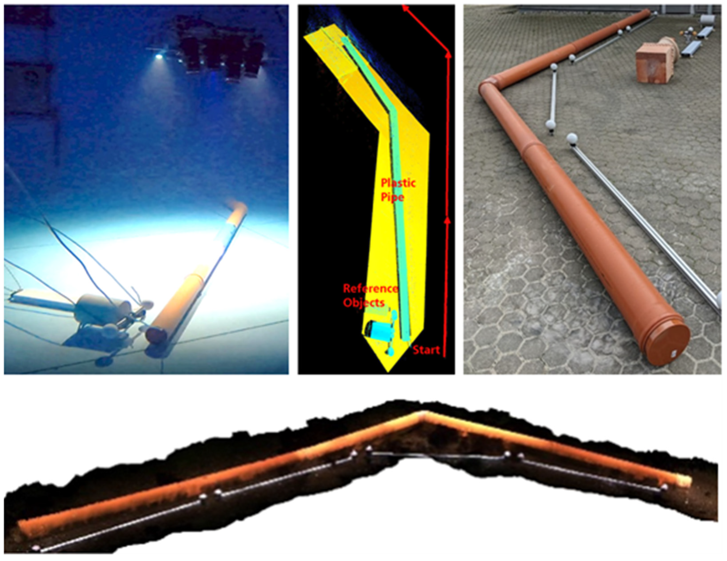
• Use case 1: The complete measurement of a “large” structure (approx. 5–10 m in diameter) on the ground with a mean scanner speed of approx. 0.5 m/s;
• Use case 2: A pipeline is traveled at a high scanner speed of approx. 1 m/s (constant) with minimal changes in direction and an average measuring distance of 2 m;
• Use case 3: The inspection of an anchor chain or similar object is carried out at a low scanner speed of approx. 0.2 m/s (constant) with minimal changes in direction.

In addition to the experimental measurements assigned to the three use cases (see Section 3.2), tests were carried out to determine the potentially achievable 3D measurement accuracy. A special experimental schedule was drawn up here. Both static measurements and those with a moving sensor system were carried out.

The further test sequences were each assigned to one of the three use cases (modes). The result of the data recording is always a 3D model of the sensor system’s surroundings scanned during the recording period. This 3D model contains both globally connected 3D data generated using visual odometry and color data with low absolute accuracy, as well as 3D data sets in high detail. A low-resolution model is generated in real-time and can be displayed by the operator or ROV pilot via a monitor with a low latency of less than 200 ms to assess the completeness of the measurement results.

Figure 7 shows the sensor system before the application and the transport of the ArUco markerboards into the water by a crane.

3.1. Evaluation Measurements

The measurements to determine the measurement accuracy are used to evaluate the calibration quality and to estimate systematic and random measurement errors in the 3D reconstruction of the underwater measurement objects. They are based on the standard for evaluating area-measuring optical sensors according to VDI/VDE [36]. This particularly concerns the determination of ball distances, the shape and dimensions of the balls, and the determination of the flatness deviation of planar measurement standards in accordance with [36].

Various experiments were carried out to determine random and systematic measurement errors for the UWS1 and UWS2 measurement systems. The studies were carried out both in clean fresh water (water basin) and in seawater (Baltic Sea). The experiments are described in detail in [32,35]. The relevant overall results are presented here. The accuracy tests were based on the VDI/VDE standard for area-measuring optical systems [36]. Length measurement errors, flatness deviations, spherical size, and shape errors, as well as measurement noise on flat and spherical surfaces, were determined. The results are documented in

Table 1. Sphere radius error, depending on the measurement distance in water basin. The calibrated radii of spheres S1 and S2 are 50.202 mm and 50.193 mm, respectively.

Distance (m)	Error S1 (mm)	Noise (mm)	Error S2 (mm)	Noise (mm)
1.5 ± 0.01	0.21 ± 0.07	0.07 ± 0.01	0.04 ± 0.01	0.07 ± 0.01
1.8 ± 0.01	0.18 ± 0.01	0.09 ± 0.01	0.02 ± 0.03	0.08 ± 0.01
2.1 ± 0.01	0.33 ± 0.01	0.09 ± 0.01	0.05 ± 0.06	0.09 ± 0.01
2.4 ± 0.01	0.37 ± 0.04	0.13 ± 0.01	0.12 ± 0.04	0.10 ± 0.01

and

Table 2. Distance-dependent flatness deviation and noise of sensor UWS1 on the normal plane in water basin.

Distance (m)	Flatness Deviation (mm)	Noise (mm)	n
1.7	0.33 ± 0.04	0.06 ± 0.01	4
2.0	0.37 ± 0.04	0.07 ± 0.01	4
2.4	0.73 ± 0.13	0.15 ± 0.02	4

. Thanks to the mechanical fixation, the measurement distance to the plane normal could be achieved without fluctuations in the water basin.

The maximal mean error of the ball-bar length measurements in the water basin was 0.53 mm, which corresponds to about 0.1%. At offshore measurements, this maximum error increased to 4.1 mm, corresponding to 0.8%.

The reason for the strong reduction in the measurement accuracy between the measurements in the water basin and the offshore measurements is likely primarily due to the poorer environmental conditions during calibration. The accuracy of recording the selected calibration points may be lower than under optimal conditions in clear fresh water. Nevertheless, it cannot be ruled out that different calibrations may turn out differently by chance. Unfortunately, due to time and capacity constraints, this could not be investigated experimentally and should be an aspect of future investigations.

Absolute measurement errors of less than 1% amount to an acceptable result when measuring lengths under relatively adverse conditions underwater.

The standard deviation of the Euclidean distance of the 3D measurement points from a fitted sphere or plane is determined as a measure of noise. This measure provides an indication of the average deviation between individual 3D measurement values and the actual values. A higher point density allows for better noise reduction through averaging. Lower noise levels enable the improved detection of fine structures, ideally close to the resolution limit.

3.2. Offshore Measurement Examples

To evaluate both 3D sensor systems, various experiments were carried out in an application-related environment in the Baltic Sea. These experiments were carried out in collaboration with the company BalticTaucher [37]. The calibration of the two sensor systems was accomplished on-site according to the method described in Section 2.2.2. For the experimental measurements, the sensor systems were mounted on a work-class ROV and controlled from a ship (see Figure 6).

As part of the experiments regarding use case 1, various measurement objects were placed in a row on the seabed, and the entire scene was reconstructed. Scanner speeds between 0.2 m/s and 0.5 m/s were achieved. The manual control of the scanner system by the ROV pilot could not achieve a constant speed.

An example of the reconstruction result of many measurement objects, including clay pots, normal planes, ball-bars, dummy bombs, and cylinders on the seabed, is shown in Figure 8.

As part of the experiments regarding use case 2, a pipe segment was reconstructed. This experiment was carried out both in the water basin and offshore. The pipe segment was placed on the bottom of the water basin or on the seabed. The test in the water basin was carried out by connecting the sensor system to a controllable traversing unit with which exact speeds could be achieved. A scanner speed of 0.7 m/s was achieved. As a result, the part of the pipe segment visible from above could be completely reconstructed (see Figure 9). When measuring offshore pipes, ball-bars were placed next to the pipe sections to determine the dimensions (see Figure 9).

Additionally, individual objects in the test row were reconstructed separately. This applies to reference measuring bodies, various clay pots, and a dummy bomb. Underwater 3D reconstruction results of one of the clay pots and the dummy bomb are documented in Figure 10 and Figure 11.

The high accuracy potential of the 3D sensor can be seen in the detailed reconstruction of the damage (long notches and grooves) on the dummy bomb. These are not measurement artifacts but are actually present on the object’s surface.

4. Discussion

In this paper, an underwater 3D sensor system is introduced, which enables high-resolution 3D capture as well as the simultaneous acquisition of color data using active stereo scanning with structured lighting, producing highly accurate and detailed 3D images for the close-range inspection of industrial structures and other objects. Three-dimensional models of industrial facilities such as piping systems, offshore wind farm foundations, anchor chains, and other structures were identified at deep depths of up to 1000 m.

The newly developed underwater sensor system enables the mobile acquisition of three-dimensional structures in real-time with a high level of detail in both clear water and natural waters such as the Baltic Sea. Up to 50 frames of 3D data can be generated per second. The high 3D measurement accuracy was largely achieved by paying particular attention to the development of the calibration process for the underwater 3D sensor system. The calibration procedure is based on the geometric modeling of visual rays, considering the refraction at media transitions. Additional refinement processes also reduce the systematic measurement error of the sensor system.

This system performs the motion estimation and correction of disturbing motion effects as well as the fusion of individual scans into a globally consistent 3D model. For mobile measurements, an improvement in the quality of the 3D point cloud was achieved through automatic motion compensation. When testing in clear water, measurement results were achieved with a very low systematic error. These errors are within the same accuracy range as measurements in air over a comparable measurement volume. The offshore measurements showed an increase in the random length measurement error with repeated measurements at the same measurement distance compared to the water basin measurement. Additionally, there was a slight scaling error of under one percent, which still represents high accuracy.

With the successful completion of the project and the realization of the two demonstrators of the deep underwater 3D sensor system, the suitability of the measurement principles used for the precise 3D surface recording and 3D modeling of underwater structures is shown. The mobile mapping of the entire covered area, e.g., the seabed, based on visual odometry was successfully demonstrated.

Unfortunately, influences caused by the vibration of the sensor support system or temperature fluctuations could not be investigated in the experiments. However, measures have already been taken to limit these influences using a carbon rod for the mechanical connection of the measuring elements and the development of a cooling system that dissipates the heat generated by the cameras and the projection unit via the housing to the surrounding water. However, it is to be expected that a potentially significant influence on measurement accuracy remains. Determining the impact of these influences on measurement accuracy should be part of future experiments.

Due to the dissimilarity compared to other optical underwater 3D measurement systems, it is difficult to make exact quantitative comparisons in terms of performance and measurement accuracy. In terms of quality, it can be said that compared to other SLAM-capable systems, e.g., the systems described in [10,38], a significantly higher level of detail can be achieved through the 3D scans from the two measuring cameras. Compared to sonar-based systems [2], the measurement accuracy is likely to be many times higher. However, the speed of large-scale acquisition and reconstruction, for example, of the seabed or a structure, is correspondingly lower.

The optical mapping system introduced by Kwasnitschka et al. [39] uses a color camera with a fisheye lens and is suitable for the extensive recording of the seabed at a depth of up to 6000 m. It can cover a much larger area than our system in a shorter time. It also enables 3D capture, although with significantly lower resolution and accuracy.

5. Conclusions

The presented 3D sensor system has high potential for use in the inspection of technical underwater structures, as well as for the detailed documentation of flooded cultural heritage sites or sunken shipwrecks. Further potential lies in the large-scale mapping of the seabed at depths of up to 1000 m in conjunction with the detailed recording of individual objects with high measurement accuracy.

In its current form, however, several improvements are desirable, primarily to make the system more manageable. This includes reducing both dimensions and mass to make the system mountable to inspection-class ROVs. Furthermore, the preparatory effort before a measurement operation, which currently requires up to a week of prearrangement time, should be reduced. In addition to structural changes to the overall system, further detailed test operations in the offshore area are necessary. Approaches have been developed by the authors to address these needs, and further development projects are being planned.

References

1. Davis, A.; Lugsdin, A. Highspeed underwater inspection for port and harbour security using Coda Echoscope 3D sonar. In Proceedings of the Oceans 2005 MTS/IEEE, Washington, DC, USA, 17–23 September 2005. [Google Scholar] [CrossRef]
2. Guerneve, T.; Pettilot, Y. Underwater 3D Reconstruction Using BlueView Imaging Sonar; IEEE: New York, NY, USA, 2015. [Google Scholar] [CrossRef]
3. ARIS-Sonars. 2022. Available online: http://soundmetrics.com/Products/ARIS-Sonars (accessed on 9 November 2023).
4. McLeod, D.; Jacobson, J.; Hardy, M.; Embry, C. Autonomous inspection using an underwater 3D LiDAR. In An Ocean in Common, Proceedings of the 2013 OCEANS, San Diego, CA, USA, 23–27 September 2013; IEEE: New York, NY, USA, 2014. [Google Scholar]
5. 3DatDepth. 2022. Available online: http://www.3datdepth.com/ (accessed on 9 November 2023).
6. Mariani, P.; Quincoces, I.; Haugholt, K.H.; Chardard, Y.; Visser, A.W.; Yates, C.; Piccinno, G.; Risholm, P.; Thielemann, J.T. Range gated imaging system for underwater monitoring in ocean environment. Sustainability 2019, 11, 162. [Google Scholar] [CrossRef]
7. Balletti, C.; Beltrane, C.; Costa, E.; Guerr, F.; Vernier, P. Underwater photogrammetry and 3D reconstruction of marble cargos shipwrecks. In Proceedings of the International Archives of the Photogrammetry, Remote Sensing and Spatial Information Sciences, Piano di Sorrento, Italy, 16–17 April 2015; pp. 7–13. [Google Scholar]
8. Zhukovsky, M.O.; Kuznetsov, V.D.; Olkhovsky, S.V. Photogrammetric techniques for 3-D underwater record of the antique time ship from from Phangoria. In Proceedings of the International Archives of the Photogrammetry, Remote Sensing and Spatial Information Sciences, Volume XL-5/W2, 2013, XXIV International CIPA Symposium, Strasbourg, France, 2–6 September 2013; pp. 717–721. [Google Scholar]
9. Vaarst. 2023. Available online: https://vaarst.com/subslam-3d-imaging-technology/ (accessed on 20 December 2023).
10. Menna, F.; Battisti, A.; Nocerino, E.; Remondino, F. FROG: A portable underwater mobile mapping system. In Proceedings of the International Archives of the Photogrammetry, Remote Sensing and Spatial Information Sciences, Padua, Italy, 24–26 May 2023; pp. 295–302. [Google Scholar] [CrossRef]
11. Tetlow, S.; Allwood, R.L. The use of a laser stripe illuminator for enhanced underwater viewing. In Proceedings of the Ocean Optics XII 1994, Bergen, Norway, 26 October 1994; Volume 2258, pp. 547–555. [Google Scholar]
12. CathXOcean. 2022. Available online: https://cathxocean.com/ (accessed on 9 November 2023).
13. Voyis. 2022. Available online: https://voyis.com/ (accessed on 9 November 2023).
14. Yousif, K.; Bab-Hadiashar, A.; Hoseinnezhad, R. An Overview to Visual Odometry and Visual SLAM: Applications to Mobile Robotics. Intell. Ind. Syst. 2015, 1, 289–311. [Google Scholar] [CrossRef]
15. Kwon, Y.H.; Casebolt, J. Effects of light refraction on the accuracy of camera calibration and reconstruction in underwater motion analysis. Sports Biomech. 2006, 5, 315–340. [Google Scholar] [CrossRef]
16. Telem, G.; Filin, S. Photogrammetric modeling of underwater environments. ISPRS J. Photogramm. Remote Sens. 2010, 65, 433–444. [Google Scholar] [CrossRef]
17. Sedlazeck, A.; Koch, R. Perspective and non-perspective camera models in underwater imaging—Overview and error analysis. In Theoretical Foundations of Computer Vision; Springer: Berlin/Heidelberg, Germany, 2011; Volume 7474, pp. 212–242. [Google Scholar]
18. Li, R.; Tao, C.; Curran, T.; Smith, R. Digital underwater photogrammetric system for large scale underwater spatial information acquisition. Mar. Geod. 1996, 20, 163–173. [Google Scholar] [CrossRef]
19. Maas, H.G. On the accuracy potential in underwater/multimedia photogrammetry. Sensors 2015, 15, 1814–1852. [Google Scholar] [CrossRef] [PubMed]
20. Beall, C.; Lawrence, B.J.; Ila, V.; Dellaert, F. 3D reconstruction of underwater structures. In Proceedings of the 2010 IEEE/RSJ International Conference on Intelligent Robots and Systems, Taipei, Taiwan, 18–22 October 2010; pp. 4418–4423. [Google Scholar]
21. Skinner, K.A.; Johnson-Roberson, M. Towards real-time underwater 3D reconstruction with plenoptic cameras. In Proceedings of the IEEE/RSJ International Conference on Intelligent Robots and Systems (IROS), Daejon, Republic of Korea, 9–14 October 2016; pp. 2014–2021. [Google Scholar]
22. Bruno, F.; Bianco, G.; Muzzupappa, M.; Barone, S.; Razionale, A.V. Experimentation of structured light and stereo vision for underwater 3D reconstruction. ISPRS J. Photogramm. Remote Sens. 2011, 66, 508–518. [Google Scholar] [CrossRef]
23. Bianco, G.; Gallo, A.; Bruno, F.; Muzzupappa, M. A comparative analysis between active and passive techniques for underwater 3D reconstruction of close-range objects. Sensors 2013, 13, 11007–11031. [Google Scholar] [CrossRef] [PubMed]
24. Luhmann, T.; Robson, S.; Kyle, S.; Harley, I. Close Range Photogrammetry; Wiley Whittles Publishing: Caithness, UK, 2006. [Google Scholar]
25. Lam, T.F.; Blum, H.; Siegwart, R.; Gawel, A. SL sensor: An open-source, ROS-based, real-time structured light sensor for high accuracy construction robotic applications. arXiv 2021, arXiv:2201.09025. [Google Scholar] [CrossRef]
26. Furukawa, R.; Sagawa, R.; Kawasaki, H. Depth estimation using structured light flow-analysis of projected pattern flow on an object’s surface. In Proceedings of the IEEE International Conference on Computer Vision, Venice, Italy, 22–29 October 2017; pp. 4640–4648. [Google Scholar]
27. Leccese, F. Editorial to selected papers from the 1st IMEKO TC19 Workshop on Metrology for the Sea. Acta IMEKO 2018, 7, 1–2. [Google Scholar] [CrossRef]
28. Gaglianone, G.; Crognale, J.; Esposito, C. Investigating submerged morphologies by means of the low-budget “GeoDive” method (high resolution for detailed 3D reconstruction and related measurements). Acta IMEKO 2018, 7, 50–59. [Google Scholar] [CrossRef]
29. Heist, S.; Dietrich, P.; Landmann, M.; Kühmstedt, P.; Notni, G. High-speed 3D shape measurement by GOBO projection of aperiodic sinusoidal fringes: A performance analysis. In Proceedings of the SPIE Dimensional Optical Metrology and Inspection for Practical Applications VII, 106670A, Orlando, FL, USA, 17–19 April 2018; Volume 10667. [Google Scholar] [CrossRef]
30. Bleier, M.; Munkelt, C.; Heinze, M.; Bräuer-Burchardt, C.; Lauterbach, H.A.; van der Lucht, J.; Nüchter, A. Visuelle Odometrie und SLAM für die Bewegungskompensation und mobile Kartierung mit einem optischen 3D-Unterwassersensor. In Photogrammetrie Laserscanning Optische 3D-Messtechnik, Beiträge der Oldenburger 3D-Tage 2022; Jade Hochschule: Wilhelmshaven, Germany, 2022; pp. 394–405. [Google Scholar]
31. Schütz, M. Potree: Rendering Large Point Clouds in Web Browsers. Bachelor’s Thesis, Technische Universität Wien, Vienna, Austria, 2015. [Google Scholar] [CrossRef]
32. Bräuer-Burchardt, C.; Munkelt, C.; Gebhart, I.; Heinze, M.; Kühmstedt, P.; Notni, G. Underwater 3D Measurements with Advanced Camera Modelling. PFG-J. Photogramm. Remote Sens. Geoinf. Sci. 2022, 90, 55–67. [Google Scholar] [CrossRef]
33. Shortis, M. Camera calibration techniques for accurate measurement underwater. In 3D Recording and Interpretation for Maritime Archaeology; Coastal Research Library; McCarthy, J., Benjamin, J., Winton, T., van Duivenvoorde, W., Eds.; Springer: Cham, Switzerland, 2019; Volume 31. [Google Scholar]
34. Kruck, E. BINGO: Ein Bündelprogramm zur Simultanausgleichung für Ingenieuranwendungen—Möglichkeiten und praktische Ergebnisse. In Proceedings of the International Archive for Photogrammetry and Remote Sensing, Rio de Janeiro, Brazil, 7–9 May 1984. [Google Scholar]
35. Bräuer-Burchardt, C.; Munkelt, C.; Bleier, M.; Heinze, M.; Gebhart, I.; Kühmstedt, P.; Notni, G. A New Sensor System for Accurate 3D Surface Measurements and Modeling of Underwater Objects. Appl. Sci. 2022, 12, 4139. [Google Scholar] [CrossRef]
36. VDI/VDE; VDI/VDE 2634. Optical 3D-Measuring Systems. In VDI/VDE Guidelines; Verein Deutscher Ingenieure: Düsseldorf, Germany, 2008. [Google Scholar]
37. Baltic Taucherei- und Bergungsbetrieb Rostock GmbH. 2023. Available online: https://baltic-taucher.com/ (accessed on 9 November 2023).
38. Rahman, S.; Quattrini Li, A.; Rekleitis, I. SVIn2: A multi-sensor fusion-based underwater SLAM system. Int. J. Robot. Res. 2022, 41, 1022–1042. [Google Scholar] [CrossRef]
39. Kwasnitschka, T.; Köser, K.; Sticklus, J.; Rothenbeck, M.; Weiß, T.; Wenzlaff, E.; Schoening, T.; Triebe, L.; Steinführer, A.; Devey, C.; et al. DeepSurveyCam—A Deep Ocean Optical Mapping System. Sensors 2016, 16, 164. [Google Scholar] [CrossRef] [PubMed]
Figure 1. Scheme of the sensor system with five tubes containing measurement cameras (Cm), color camera (Ccol), IMU (I), projection unit (P), and electronic control box (E). Additionally, two flashlights (F) are mounted on the carbon fiber rod (R).
Applsci 14 00557 g001
Figure 2. Software architecture.
Applsci 14 00557 g002
Figure 3. Two examples of the graphical user interface of the monitoring software: a scenic view with different lighting and contrast levels, a histogram equalization sketch (above), and a 3D point of view with latency display (below); blue boxes are added for explanation.
Applsci 14 00557 g003
Figure 4. ArUco markerboards for calibration.
Applsci 14 00557 g004
Figure 5. Reference bodies’ ball-bar and cylinder (left), 3D reconstruction result without (middle) and with motion compensation (right).
Applsci 14 00557 g005
Figure 6. UWS mounted on ROV immediately before measurement application (a) and control room for UWS and ROV on the ship (b).
Applsci 14 00557 g006
Figure 7. UWS mounted on ROV (a) and placement of the ArUco markerboards into the water (b).
Applsci 14 00557 g007
Figure 8. Reconstruction result of line of test objects using visual odometry and color mapping.
Applsci 14 00557 g008
Figure 9. Reconstruction results of a pipe section: measurement in the water basin, reconstruction result water basin, pipe for underwater measurement in air (from left to right above), and underwater reconstruction result for offshore measurement (below).
Applsci 14 00557 g009
Figure 10. Photograph (left), 3D reconstruction result obtained via VO (middle) with mapped color information (right) of a clay pot.
Applsci 14 00557 g010
Figure 11. Photograph of three dummy bombs and the 3D reconstruction result of one of the bombs.
Applsci 14 00557 g011