Allocation and Sizing of DSTATCOM with Renewable Energy Systems and Load Uncertainty Using Enhanced Gray Wolf Optimization

Abstract

Over the last decade, flexible alternating current transmission systems (FACTS) have been crucial in ensuring optimal power distribution within modern power systems. A vital component of FACTS devices is the distribution static compensator (DSTATCOM), which is essential for maintaining a reliable power supply. It is commonly used for reactive power compensation, voltage regulation, and harmonic reduction. Determining the appropriate size and placement of DSTATCOMs is vital to ensuring their efficiency. This study introduces the improved gray wolf optimizer (I-GWO), a refined version of the classical gray wolf optimization (GWO) method. The I-GWO incorporates a dimension learning-based hunting (DLH) strategy to preserve population diversity, balance exploration and exploitation, and prevent the premature convergence of classical GWO. In this research, the I-GWO was applied to determine the optimum allocation and sizing of the DSTATCOMs, considering system constraints, including those presented by the intermittent and stochastic nature of the load and renewable energy resources, specifically wind and solar energy. The suggested approach was successfully tested on 33-, 69-, and 85-bus distribution systems and then compared with existing studies. The results demonstrated the I-GWO-based approach’s superiority in terms of reducing power losses, improving voltage profiles, and enhancing voltage stability.

1. Introduction

Load growth in distribution systems can lead to increased power losses, a reduced voltage profile, financial losses for utility companies, and voltage stability problems. Voltage instability, if not addressed, may eventually lead to system collapse. One solution that has been proposed is shunt compensation [1,2], which involves using devices such as capacitors and inductors to balance the reactive power in the system. However, shunt compensation can also lead to resonance problems.

The distribution static compensator (DSTATCOM) has emerged as a vital solution for power distribution systems. It was initially designed to address transient anomalies- such as voltage sags, swells, and other disturbances within the distribution network. Modern applications have tapped into the DSTATCOM’s steady-state operations capabilities to reduce power losses, enhance voltage stability, and improve voltage profiles. Compared with conventional capacitor compensators, the DSTATCOM offers superior flexibility by providing lagging and leading reactive power. It responds instantly to disturbances, delivering rapid voltage regulation and continuous reactive power support. Beyond these benefits, the DSTATCOM can also mitigate harmonics, elevate overall power quality, and buttress the system voltage during faults. In contrast to capacitor banks that may introduce resonance challenges, the DSTATCOM operates without such resonance risks. Its compact dimensions demand minimal space, and its solid-state composition guarantees diminished maintenance needs and a prolonged operational lifespan. However, ensuring that the DSTATCOM is optimally sized and allocated within the radial distribution system is imperative. Inappropriate size or placement can have negative impacts, potentially undermining the benefits it offers.

Recently, many algorithms have been developed for the optimum allocation and sizing of DSTATCOMs in power distribution systems. Most of these algorithms employ metaheuristic techniques. Such methods are renowned for finding global solutions, avoiding becoming trapped in local minima, and rapidly searching large solution spaces. Examples include the differential evolution algorithm (DEA) [3], particle swarm optimization (PSO) [4], genetic algorithms (GA) [5], immune algorithm (IA) [6], lightning search algorithm (LSA) [7], bat algorithm (BA) [8], bacterial foraging optimization algorithm (BFOA) [9], and cuckoo search algorithm (CSA) [10], as well as the multi-objective sine-cosine approach (MOSCA) and multi-objective particle swarm optimization (MOPSO), which are both discussed in Reference [11]. Most existing research does not consider the presence of renewable energy sources and load fluctuations. These factors introduce intermittency and uncertainty, significantly impacting the load flow of the power system. The main contributions of this study are:

• Introducing a new method for the optimal allocation and sizing of DSTATCOMs in radial distribution systems.
• Incorporating the uncertainty associated with load fluctuations and renewable energy generation into the DSTATCOM allocation and sizing process.

The gray wolf optimizer (GWO) [12] is a metaheuristic bio-inspired algorithm based on gray wolves’ hunting and leadership hierarchy behavior in their natural environment. This algorithm incorporates four main decision variables, represented by the roles of the wolves: alpha (leader of the pack), beta (second-in-command after the leader), delta (third in order), and omega (the lowest-ranking members of a wolf pack). The efficacy of this approach has been proven by effectively dealing with a wide array of optimization challenges, including domains such as engineering design, machine learning, and image processing. Building on this foundation, a previous study [13] introduced the improved gray wolf optimizer (I-GWO), an enhanced version of the GWO designed explicitly for solving global optimization problems and engineering tasks. The I-GWO integrates the dimension learning-based hunting (DLH) strategy, aiming to address the inherent limitations of the GWO, such as insufficient population diversity, the lack of balance between exploration and exploitation, and premature convergence.

In the present paper, the I-GWO algorithm is used to allocate optimally and to size multiple DSTATCOMs in distribution systems, while considering the uncertainty of load and renewable resource generation. To demonstrate its efficiency, the approach is tested on several test systems, including the IEEE-33 bus, IEEE-69 bus, and IEEE-85 radial distribution systems. Moreover, the developed method is compared with BFOA [9], CSA [10], LSA [7], MOPSO, and MOSCA [11] to illustrate its superiority in terms of reducing power losses, improving voltage profiles, and enhancing voltage stability.

The remaining sections of the present paper are structured as follows: Section 2 covers the mathematical formulation and modeling of the problem. Section 3 discusses the modeling of renewable energy resources. Section 4 details the proposed optimization method, I-GWO. Section 5 presents the application of I-GWO to the proposed problem. In Section 6, the obtained results are presented and analyzed, along with a commentary. Lastly, our conclusions are presented in Section 7.

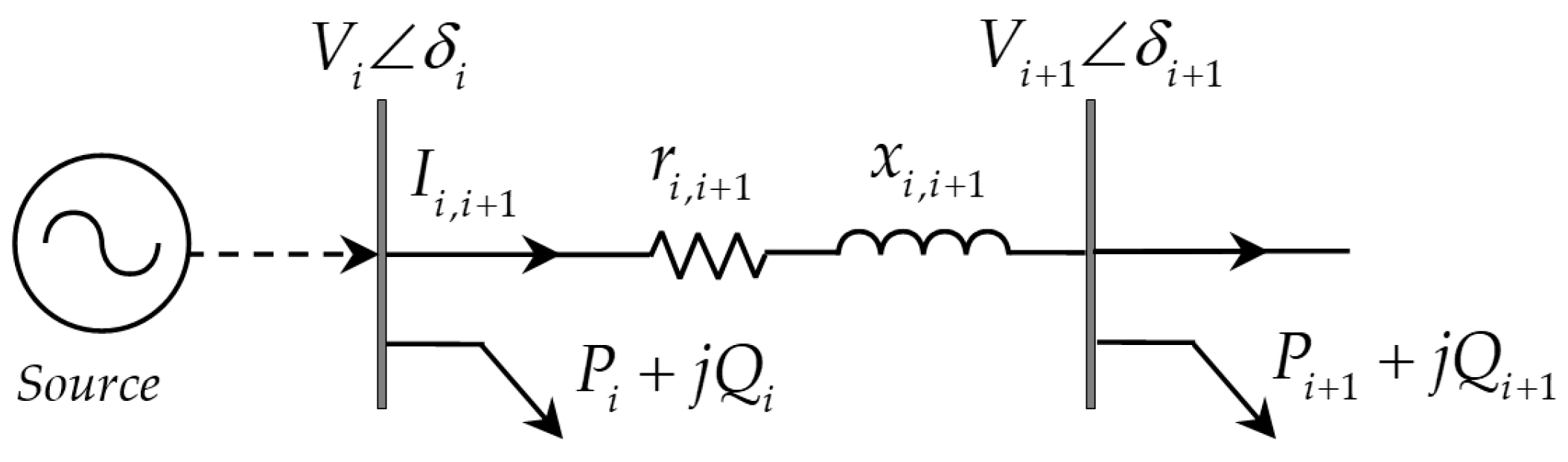
2. Problem Formulation

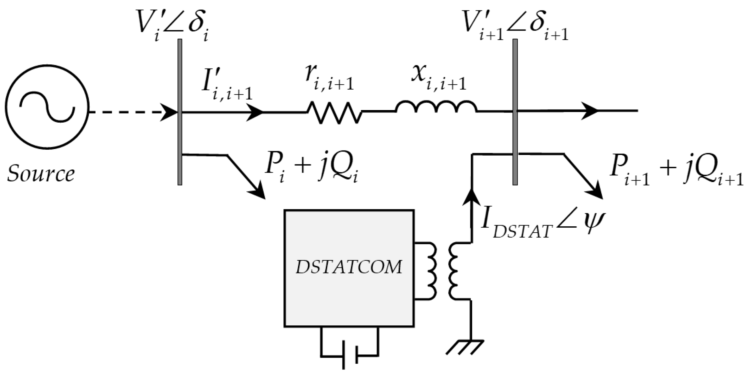
2.1. Modeling of DSTATCOM

In radial distribution systems, each receiving bus is supplied by a single sending bus. Figure 1 illustrates a section wherein the DSTATCOM is planned to be installed:

The voltage value at the receiving node is computed using Kirchhoff’s voltage law (KVL), as follows:

$$V_{i+1}\angle {\theta }_{i+1}=V_i\angle {\theta }_i-\left(r_{i,i+1}+j{x}_{i,i+1}\right)I_{i,i+1}\angle {\delta }_{i,i+1}$$

(1)

where the bus voltages for nodes $i$ and $i+1$ are represented by $V_i$ and $V_{i+1}$, and the associated phase angles for these nodes are given by ${\theta }_i$ and ${\theta }_{i+1}$. $I_{i,i+1}$ represents the current flowing from node $i$ to node $i+1$, and its phase angle is denoted by ${\delta }_{i,i+1}$. The resistance and reactance for this branch are indicated by $r_{i,i+1}$ and $x_{i,i+1}$, respectively.

After the DSTATCOM installation, the candidate bus’s voltage profile and all other buses will change to a new value, as shown in Figure 2.

Consequently, the updated KVL equation for the compensated bus may be expressed as follows:

$${V^{\prime }}_{i+1}\angle {{\theta }^{\prime }}_{i+1}=V_i{}^{}\angle {\theta }_i{}^{}-\left(r_{i,i+1}+j{x}_{i,i+1}\right)\times \left[I_{i,i+1}\angle {\delta }_{i,i+1}+I_{DSTAT}\angle \psi \right]$$

(2)

The DSTATCOM may generate or consume reactive power but does not contribute to active power in steady-state conditions. Consequently, the current injected by the DSTATCOM is in quadrature with the voltage of the compensated bus. This relationship is illustrated in the Vector Representation of Voltage and Current Phasors shown in Figure 3. The correlation can also be expressed in the following equation:

$$\psi ={{\theta }^{\prime }}_{i,i+1}+\frac{\pi }{2}$$

(3)

In this study, DSTATCOM is treated as a current source. When the voltage magnitude of the DSTATCOM is greater than that of the compensated node, the current flows toward the node. Conversely, if the voltage magnitude of the DSTATCOM is less than the compensated node’s voltage, the current flows in the opposite direction. The expression for the injected current of the DSTATCOM is expressed as follows:

$$I_{DSTAT}={\left(\frac{-j{Q}_{DSTAT}}{V_{DSTAT}}\right)}^{*}=\left|\frac{Q_{DSTAT}}{V_{DSTAT}}\right|\angle {{\theta }^{\prime }}_{i,i+1}+\frac{\pi }{2}$$

(4)

Assuming the magnitude of the DSTATCOM voltage $V_{DSTAT}$ to be 1.0 p.u., the only unknown variable in Equation (4) is ${{\theta }^{\prime }}_{i,i+1}$. Determining its value requires substituting Equation (4) into Equation (2). After some algebraic manipulations [14], the result is:

$$X_1=\left[\frac{K_1\left(1-C_2\left|\frac{Q_{DSTAT}}{V_{DSTAT}}\right|\right)+K_2{C}_1\left|\frac{Q_{DSTAT}}{V_{DSTAT}}\right|}{{\left(1+C_2\left|\frac{Q_{DSTAT}}{V_{DSTAT}}\right|\right)}^2+C_1{C}_2{\left|\frac{Q_{DSTAT}}{V_{DSTAT}}\right|}^2}\right]\times \left[\frac{1}{{V^{\prime }}_{i+1}}\right]$$

(5)

$$X_2=\left[\frac{K_2\left(1+C_2\left|\frac{Q_{DSTAT}}{V_{DSTAT}}\right|\right)+K_2{C}_1\left|\frac{Q_{DSTAT}}{V_{DSTAT}}\right|}{{\left(1+C_2\left|\frac{Q_{DSTAT}}{V_{DSTAT}}\right|\right)}^2+C_1{C}_2{\left|\frac{Q_{DSTAT}}{V_{DSTAT}}\right|}^2}\right]\times \left[\frac{1}{{V^{\prime }}_{i+1}}\right]$$

(6)

where:

$K_1=\Re e\left\{{V^{\prime }}_{i,i+1}\angle {{\theta }^{\prime }}_{i,i+1}-\left(r_{i,i+1}+j{x}_{i,i+1}\right)\times {I^{\prime }}_{i,i+1}\angle {\delta }_{i,i+1}\right\}$

$K_2=\Im m\left\{{V^{\prime }}_{i,i+1}\angle {{\theta }^{\prime }}_{i,i+1}-\left(r_{i,i+1}+j{x}_{i,i+1}\right)\times {I^{\prime }}_{i,i+1}\angle {\delta }_{i,i+1}\right\}$

$C_1=-r_{i,i+1}, C_2=-x_{i,i+1}.$

The value of ${{\theta }^{\prime }}_{t+1}$ may be determined by using either Equation (7) or Equation (8).

$${{\theta }^{\prime }}_{t+1}={\cos }^{-1}(X_1)$$

(7)

$${{\theta }^{\prime }}_{t+1}={\sin }^{-1}(X_2)$$

(8)

2.2. Voltage Stability Index (VSI)

The evaluation of static voltage stability requires the calculation of a significant metric known as the voltage stability index (VSI), which serves as an appropriate indicator of the proximity of the power system to voltage collapse. Various techniques exist for calculating this index, including the VSI-index proposed in [15]. From Figure 1:

$${\left(V_i\angle {\theta }_i\right)}^{\ast }\cdot I_{i,i+1}=P_i-j{Q}_i$$

(9)

Based on Equations (9) and (1), we obtain the following:

$$V_i^2-V_i\cdot V_{i-1}+\sqrt{\left(P_i^2+Q_i^2\right)\cdot \left(r_{i,i-1}^2+x_{i,i-1}^2\right)}=0$$

(10)

The roots of Equation (10) are real if:

$$V_{i-1}^2-4\cdot \sqrt{\left(P_i^2+Q_i^2\right)\cdot \left(r_{i,i-1}^2+x_{i,i-1}^2\right)}\ge 0$$

(11)

Using the previous equation, the stability index for the ith bus is derived as follows:

$$VS{I}_i=V_{i-1}^4-4\cdot {\left(P_i{x}_{i,i-1}-Q_i{r}_{i,i-1}\right)}^2-4\cdot {\left(P_i{r}_{i,i-1}+Q_i{x}_{i,i-1}\right)}^2\cdot V_{i-1}^2\ge 0$$

(12)

The stability threshold of this index varies from one to zero. The bus with the minimum value is the one most sensitive to voltage collapse.

2.3. DSTATCOM-Integrated Load Flow Steps

The goal of load flow in a power system is to determine the steady-state voltages, currents, and power flows in all branches and nodes of the system under a given set of load and generation conditions. The classical load flow techniques, such as the Newton–Raphson and Gauss–Seidel methods, are not well-suited for solving load flow problems in radial distribution systems (RDS), due to the high R/X ratios inherent in these systems. In contrast, the forward-backward sweep algorithm [16], which is based on the fundamental principles of Kirchhoff’s laws, can be employed to determine the system’s power flow.

From Figure 1, the current flowing in the branch between nodes $i$ and $i+1$ is given by:

$$I_{i,i+1}=\frac{P_i-j{Q}_i}{V_i\angle -{\delta }_i}$$

(13)

Active and reactive losses within the branch are given by:

$$\{\begin{array}{l}{P}_{l(i,i+1)}=r_{i,i+1}\frac{\left(P_i^2+Q_i^2\right)}{V_i^2}\\ Q_{l(i,i+1)}=x_{i,i+1}\frac{\left(P_i^2+Q_i^2\right)}{V_i^2}\end{array}$$

(14)

The active and reactive powers at the beginning of the branch are given by:

$$\{\begin{array}{l}{P}_i=P_{i+1}+P_{l(i,i+1)}\\ Q_i=Q_{i+1}+Q_{l(i,i+1)}\end{array}$$

(15)

Considering Equations (14) and (15):

$$I_{i,i+1}=\frac{V_i\angle {\delta }_i-V_{i+1}\angle {\delta }_{i+1}}{r_{i,i+1}+j{x}_{i,i+1}}=\frac{P_i-j{Q}_i}{V_i\angle -{\delta }_i}$$

(16)

Separating the real and imaginary parts:

$$\{\begin{array}{l}{V}_i^{}{V}_{i+1}^{}\cos ({\delta }_{i+1}-{\delta }_i)=V_i^2-\left(P_i{r}_{i-1,i}+Q_i{x}_{i-1,i}\right)\\ V_i^{}{V}_{i+1}^{}\sin ({\delta }_{i+1}-{\delta }_i)=Q_i{r}_{i-1,i}-P_i{x}_{i-1,i}\end{array}$$

(17)

From Equation (17):

$$V_{i+1}={\left\{V_i^2-2\left(P_i{r}_{i+1}+Q_i{x}_{i+1}\right)+\left(r_{i,i+1}^2+x_{i,i+1}^2\right)\frac{\left(P_i^2+Q_i^2\right)}{V_i^2}\right\}}^{1/2}$$

(18)

$${\delta }_{i+1}={\delta }_i+{\tan }^{-1}\left\{\frac{Q_i{r}_{i,i+1}-P_i{x}_{i,i+1}}{V_i^2-\left(P_i{r}_{i,i+1}+Q_i{x}_{i,i+1}\right)}\right\}$$

(19)

The forward-backward sweep algorithm operates through the following steps:

• Step 1: Preparation—Read system data, including the system’s topology, bus characteristics, branch parameters, load consumption values, and DSTATCOM data, along with its operating constraints.
• Step 2: Initialization—Assume a flat voltage profile as the starting point for the initial voltages and set the first iteration, denoted as $k$, to 0.
• Step 3: Nodal Current Calculation—Calculate the injected current at each load bus $i$ using the assumed known voltage, with the following equation:

$$I_i^{(k)}=conj\left(\frac{P_{L,i}+j{Q}_{L,i}}{V_i^{(k-1)}}\right)+\left(\frac{j{B}_i}{2}{V}_i^{(k-1)}\right)$$

(20)

$B_i$ is the susceptance, where $P_{L,i}$ and $Q_{L,i}$ are the active and reactive load demands, and $V_i^{(k-1)}$ is the bus voltage at the ${\left(k-1\right)}^{th}$ iteration.

• Step 4: Adding Current Injected by the DSTATCOM—For each bus where the DSTATCOM is connected, calculate the current it injects using Equation (4). Then, add this calculated current to the previously injected current on the same bus.

$$I_i^{(k)}=I_i^{(k)}+I_{DSTAT}$$

(21)

• Step 5: Backward Sweep—Starting with the last-ordered branch, the current $J_{i+1}^{(k)}$ flowing between the node $i$ and its preceding node $i-1$ is determined using the BIBC (branch-current to bus-current) matrix [16], as follows:

$$J_{i,i-1}^{(k)}=\left[BIBC\right]\times \left[I_i^{(k)}\right]$$

(22)

• Step 6: Forward Sweep—The node voltages are updated iteratively, starting from the root bus, in accordance with the following equation:

$$V_{i+1}^{(k)}=V_i^{(k)}-Z_{i,i+1}{J}_{i,i-1}^{(k)}$$

(23)

where $Z_{i,i+1}$ is the series impedance of branch $i$, $i+1$.

• Step 7: Convergence Check—Repeat Step 5 and Step 6 until the difference in voltage magnitudes between successive iterations at each node falls below a predefined tolerance limit, as follows:

$$\max (V_{}^{(k)}-V_{}^{(k-1)})<\epsilon$$

(24)

• Step 8: Displaying Results—Using the converged voltages, calculate the branch currents with Ohm’s and Kirchhoff’s laws. Compute the active power losses in each branch and sum them to calculate the total losses.

3. Renewable Energy Resource Modeling

The increasing usage of renewable energy sources (RESs) in modern power systems introduces several challenges, due to the uncertainty of these sources [17,18]. The RESs can work in standalone mode, grid-connected mode, microgrid mode, etc. [17,18].

3.1. Wind Power Generators

Unlike traditional generators, the output of wind power generators (WPG) is unpredictable because of fluctuations in wind energy. Such randomness in the production of WPG contributes to uncertainties in power flows and losses [17]. The power output, denoted by $P_{wt}^{}$ can be mathematically expressed as a function of wind speed in the following way [17]:

$$P_{wt}(v_s)=\{\begin{array}{l}0,\hspace{1em}\hspace{0.17em}if\hspace{0.17em}\hspace{0.17em}{v}_s<v_{cut-in}\hspace{0.17em}or\hspace{0.17em}\hspace{0.17em}{v}_s>v_{cut-out}\\ P_{wt}^{rated}\times \left(\frac{v_s-v_{cut-in}}{v_{rated}-v_{cut-in}}\right)\hspace{0.17em},\hspace{0.17em}\hspace{0.17em}\hspace{0.17em}if\hspace{0.17em}{v}_{cut-in}\le v_s\le v_{rated}\hspace{0.17em}\\ P_{wt}^{rated},\hspace{0.17em}\hspace{0.17em}\hspace{0.17em}if\hspace{0.17em}\hspace{0.17em}{v}_{rated}\le v_s\le v_{cut-out}\hspace{0.17em}\end{array}$$

(25)

where $P_{wt}^{rated}$ is the rated power of the installed WPG in (MW), $v_s$ is the wind speed, $v_{rated}$ is the rated speed (m/s), $v_{cut-in}$ is the lowest wind speed at which the WPG will begin to generate power, and $v_{cut-out}$ is the maximum wind speed at which a WPG is designed to operate safely. When the wind speed $v_s$ is within the range of $v_{cut-in}$ and $v_{rated}$, the power output of the WPG increases linearly as the wind speed increases.

3.2. Solar Power Generators

Unlike wind power, solar power generators (SPG) rely on the availability and intensity of sunlight, which varies throughout the day and is influenced by weather conditions and geographical location. This inconsistency in solar irradiance gives rise to variations in power output, affecting power flows, stability, and power losses in the distribution system. The power delivered by SPG, denoted by $P_{pv}$, can be mathematically formulated as a function of solar irradiation, as follows [17]:

$$P_{pv}\left(G_s\right)=\{\begin{array}{l}{P}_{pv}^{rated}\times \left(\frac{G_s^2}{G_{std}{R}_c}\right)\hspace{1em}if 0<G_s<R_c\hfill \\ P_{pv}^{rated}\times \left(\frac{G_s}{G_{std}}\right)\hspace{1em}if G_s\ge R_c\hfill \end{array}$$

(26)

where $P_{pv}^{rated}$ is the rated power of the installed SPG in (MW), $G_s$ is the solar irradiation in W/m², $G_{std}$ is the standard solar irradiance, and $R_c$ is the irradiation threshold.

3.3. Fast Scenario Reduction Method

The data used in this work, including load levels, solar irradiance, and wind speed, are presented in Figure 4, Figure 5 and Figure 6 and are sourced from Reference [18]. This dataset contains hourly values for an entire year, resulting in 8760 data points for each variable. Figure 7 presents a focused view of the data, illustrating the variations recorded over a single day. Handling such a large volume of data presents numerous challenges [18], and scenario reduction is one of the techniques employed to deal with this complexity. Among the various reduction methods available, the fast scenario reduction (FSR) method [19] is chosen in this paper for its efficiency, reliability, and ability to select a smaller set of representative scenarios from a large set while preserving the original set’s statistical properties. The procedure of the FSR technique can be expressed in terms of the following steps, with the goal of reducing the number of scenarios from $N_s$ to $N_s^{*}$.

Step 1:

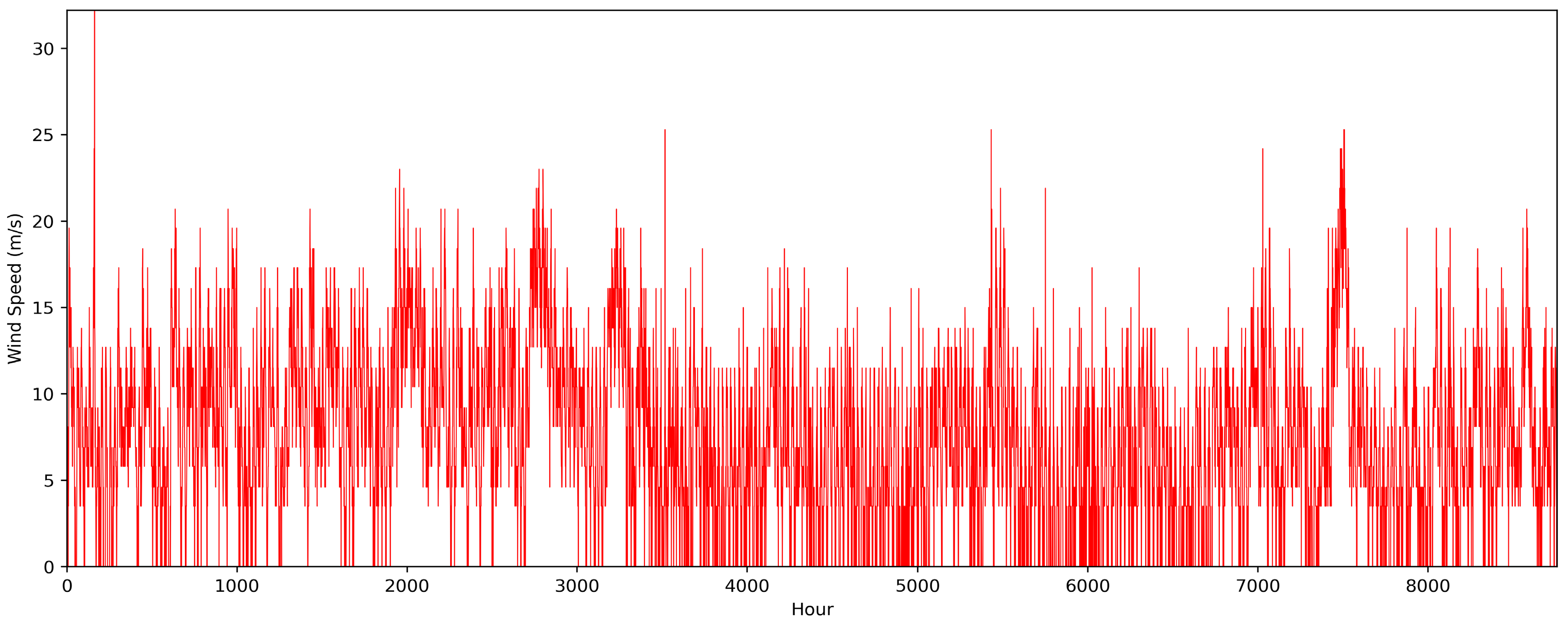
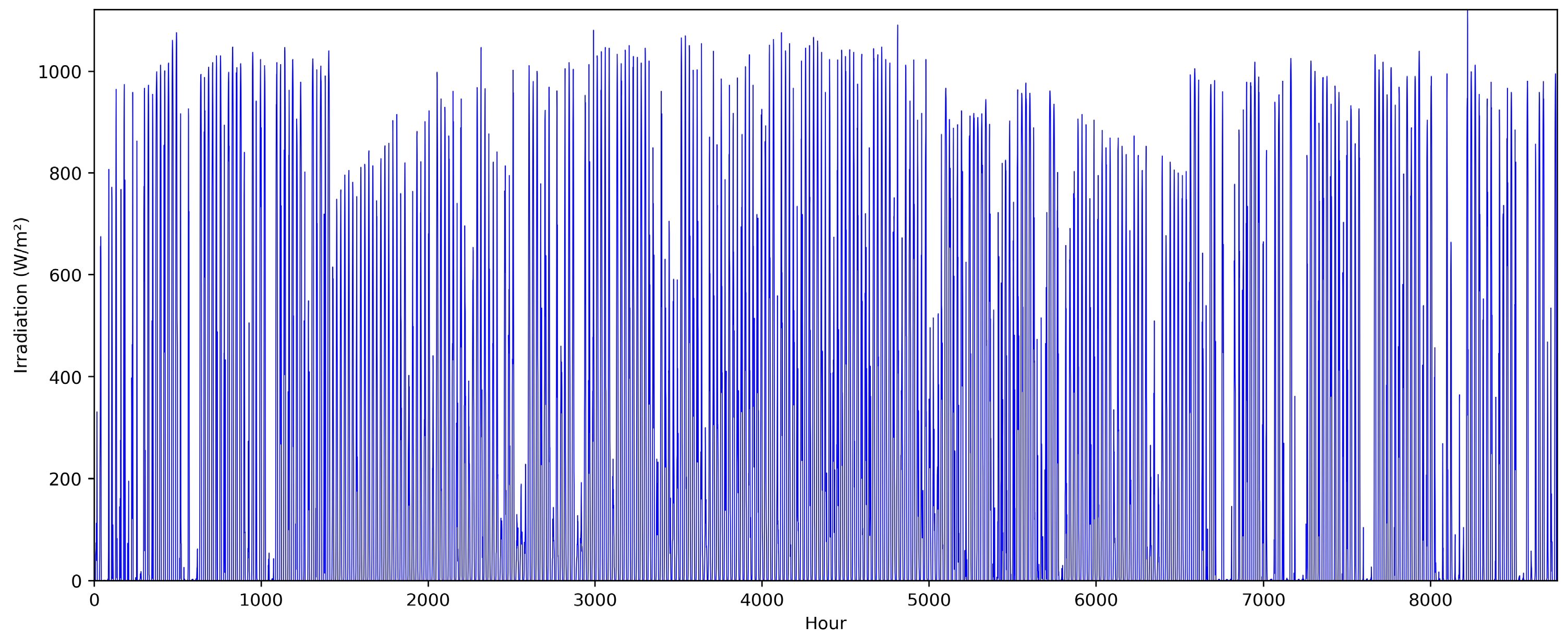
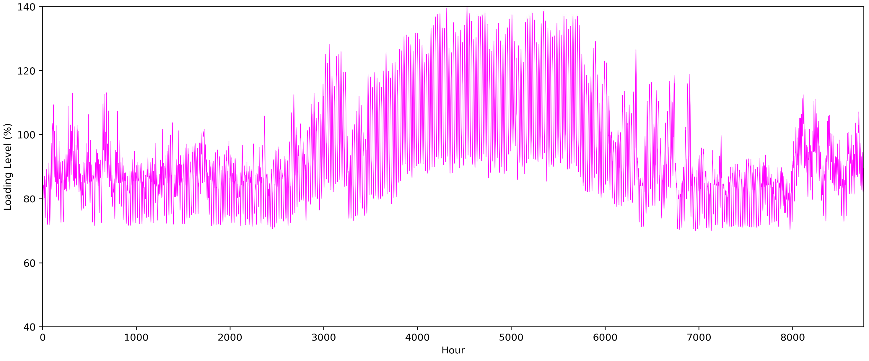
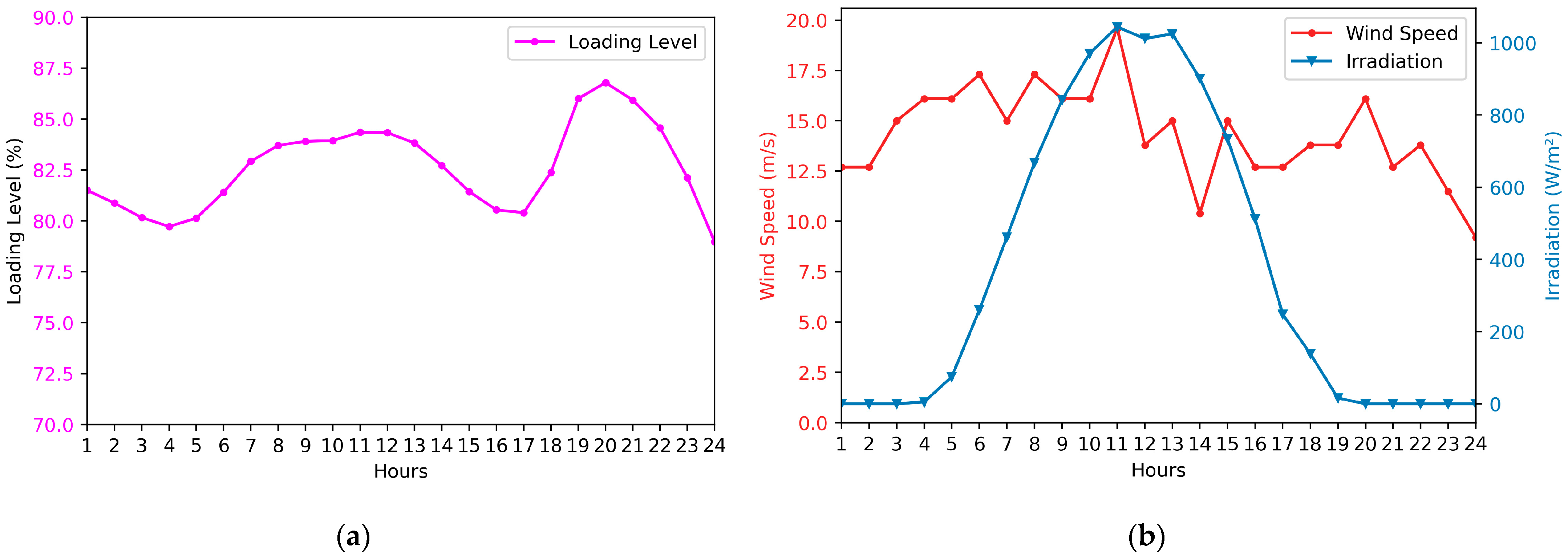
Scenario Generation—Start by generating a large set of scenarios using methods like Monte Carlo simulations, historical data, or other suitable techniques. Organize these scenarios into a matrix, denoted as $S$, where each row $s_i$ represents a scenario containing the loading level $L{L}_i$, the irradiance $G_i$, and the wind speed $v_i$, as follows:

$$S=\left[\begin{array}{ccc}L{L}_1^{}& G_1& v_1\\ ⋮& ⋮& ⋮\\ L{L}_i^{}& G_i& v_i\\ ⋮& ⋮& ⋮\\ L{L}_{Ns}^{}& G_{Ns}^{}& v_{Ns}\end{array}\right]\begin{array}{c}\leftarrow s_1\\ \\ \leftarrow s_i\\ \\ \leftarrow s_{Ns}\end{array}$$

(27)

Step 2:

Additionally, initialize the probability of each scenario to ${\tau }_i=1/N_s$, where $N_s$ represents the total number of scenarios.

Step 3:

Distance Calculation—Calculate distances between each pair of scenarios $s_i$ and $s_j$, using an appropriate measure to form a distance matrix. In this paper, the Euclidean distance with the 2-norm is adopted, and can be expressed as follows:

$$d(s_i,s_j)=\sqrt{{\left(L_i-L_j\right)}^2+{\left(G_i-G_j\right)}^2+{\left(G_i-G_j\right)}^2}$$

(28)

Step 4:

Scenarios Merging—Identify the pair of scenarios $s_i$ and $s_j$ that have the smallest Euclidean distance, as calculated in Step 2. Merge these two scenarios into a single representative scenario, often by taking the weighted average, based on their probabilities. The new scenario’s values for loading, irradiance, and wind speed can be computed as:

$$\{\begin{array}{l}L{L}_{new}=\left(L{L}_i+L{L}_j\right)/2\hfill \\ G_{new}=\left(G_i+G_j\right)/2\hfill \\ v_{new}=\left(v_i+v_j\right)/2\hfill \end{array}$$

(29)

Also, update the probability of the merged scenario ${\tau }_{new}={\tau }_i+{\tau }_j$ and decrease the number of scenarios $N_s$ by 1.

Step 5:

Termination Check—Determine if the stopping criterion has been met (e.g., by reaching a predefined tolerance level or desired number of scenarios $N_s^{*}$); otherwise, return to Step 2.

In this paper, the scenario reduction process is applied to a timescale representing the total number of hours in a year, resulting in an initial set of $N_s^{}=8760$ scenarios. The chosen number of reduced scenarios, after applying the FSR method, is $N_s^{*}=15$.

Table 1. Summary of reduced scenarios and probabilities.

Scenario	Loading Level (%)	Solar Irradiance (W/m2)	Wind Speed (m/s)	Probability τs
1	93.310	18	5.8	0.044
2	96.237	770	13.8	0.037
3	101.527	366	6.9	0.034
4	96.254	955	10.4	0.041
5	101.270	190	11.5	0.040
6	100.379	555	6.9	0.029
7	85.263	1	6.9	0.258
8	101.718	91	6.9	0.062
9	101.425	859	10.4	0.044
10	103.318	664	9.2	0.037
11	103.181	460	10.4	0.037
12	102.005	269	10.4	0.039
13	93.310	18	5.8	0.044
14	96.237	770	13.8	0.037
15	101.527	366	6.9	0.034

presents the obtained scenarios, including specific details for each scenario $s$ such as the loading level, solar irradiance, wind speed, and their corresponding probabilities (${\tau }_s$).

4. Improved Gray Wolf Optimization

The GWO method involves an optimization algorithm that takes inspiration from the structure and hunting behavior of wolves in nature [12,20,21]. In this algorithm, packs of wolves represent solutions to an optimization problem. It mimics the roles of dominant wolves (alpha, beta, and delta) in guiding the hunt, while the remaining wolves play the role of omegas. As the iterations progress, these wolves adjust their positions based on the guidance provided by the others, eventually leading to near-optimal solutions. GWO is particularly effective in exploring problems ranging from engineering design to biology.

Figure 8 illustrates the hunting strategy of gray wolves. This encircling action can be simulated using the following equations:

$$\overrightarrow{X}(t+1)=\overrightarrow{X_p}(t)-\overrightarrow{A}\cdot \left|\overrightarrow{C}\overrightarrow{X_p}(t)-\overrightarrow{X}\right|$$

(30)

$$\overrightarrow{A}=2\overrightarrow{a}\times ran{d}_1-\overrightarrow{a}$$

(31)

$$\overrightarrow{C}=2\times ran{d}_2$$

(32)

Here, $\overrightarrow{X}$ is the position vector of the prey, $\overrightarrow{X_p}$ is the position vector of a gray wolf, $\overrightarrow{A}$ and $\overrightarrow{C}$ are coefficient vectors, and $ran{d}_1,\hspace{0.17em}\hspace{0.17em}ran{d}_2$ are random values in [0, 1]. The variable $\overrightarrow{a}$ linearly decreases as the algorithm progresses through iterations, as follows:

$$\overrightarrow{a}=2-t/t_{\max }$$

(33)

where $t$ represents the current iteration and $t_{\max }$ represents the maximum number of iterations. It is worth mentioning that every mega wolf needs to simultaneously adjust its position in relation to the alpha, beta, and delta wolves, as described below:

$$\{\begin{array}{l}\overrightarrow{D_{\alpha }}=\left|\overrightarrow{C_1}\overrightarrow{X_{\alpha }}(t)-\overrightarrow{X}\right|\\ \overrightarrow{D_{\beta }}=\left|\overrightarrow{C_2}\overrightarrow{X_{\beta }}(t)-\overrightarrow{X}\right|\\ \overrightarrow{D_{\delta }}=\left|\overrightarrow{C_3}\overrightarrow{X_{\delta }}(t)-\overrightarrow{X}\right|\end{array}$$

(34)

$$\{\begin{array}{l}\overrightarrow{X_1}=\overrightarrow{X_{\alpha }}-\overrightarrow{A_1}\cdot \left(\overrightarrow{D_{\alpha }}\right)\\ \overrightarrow{X_2}=\overrightarrow{X_{\beta }}-\overrightarrow{A_2}\cdot \left(\overrightarrow{D_{\beta }}\right)\\ \overrightarrow{X_3}=\overrightarrow{X_{\delta }}-\overrightarrow{A_3}\cdot \left(\overrightarrow{D_{\delta }}\right)\end{array}$$

(35)

$$\overrightarrow{X}(t+1)=\left(\overrightarrow{X_1}+\overrightarrow{X_2}+\overrightarrow{X_3}\right)/3$$

(36)

It is noteworthy that both exploration and exploitation play vital roles in metaheuristic algorithms. GWO seeks to strike a balance between these two phases. In GWO, the value of $\overrightarrow{a}$ decreases with each iteration from 2 to 0, as represented by Equation (33). Concurrently, the $\overrightarrow{A}$ value is also reduced by $\overrightarrow{a}$, as demonstrated by Equation (31). For a gray wolf, trying to minimize the $\overrightarrow{A}$ value holds significance. When $\overrightarrow{\left|A\right|}$ is less than 1, it prompts the wolves to attack the prey. Conversely, when $\overrightarrow{\left|A\right|}$ is greater than 1, the wolves attempt to seek other prey. This behavior exemplifies the principles of exploration and exploitation. In a previous study [13], the improved gray wolf optimizer (I-GWO) was introduced as an enhanced version of the GWO for global optimization and engineering tasks. The I-GWO incorporates the dimension learning-based hunting (DLH) strategy to overcome the limitations of GWO, such as a lack of population diversity, the exploitation–exploration imbalance, and premature convergence. When evaluated against benchmark tests, the I-GWO algorithm was found to be competitive, frequently outperforming other algorithms in terms of efficiency and applicability. For more details about the method, refer to [13]. The main code for I-GWO is hosted on MathWorks and can be accessed from the following link [22].

5. Application of I-GWO to the Proposed Problem

5.1. Problem Formulation

The objective of the DSTATCOM placement and sizing problem considered in this paper is the maximization of TACS while enhancing the voltage profile.

The investment cost of the DSTATCOM per year [23] is computed as below:

$$IC{D}_{year}=CD\frac{{\left(1+B\right)}^n\times B}{{\left(1+B\right)}^n-1}$$

(37)

where $CD$ is the cost of the DSTATCOM, $B$ is the rate of return, and $n$ is the lifetime of the DSTATCOM in years. In this paper: $CD=50\$/\mathrm{kVAr},n=1,$ and $B=0.1$.

To calculate the total annual cost savings (TACS) [23], the overall energy loss costs before and after the installation of the DSTATCOM must be considered, as follows:

$$TACS=K_P\left(T\times P_{TLoss}^{Before}\right)-K_P\left(T\times P_{TLoss}^{After}\right)-\left(IC{D}_{year}\right)$$

(38)

where $K_P$ is the energy cost of losses and is given a value of $0.06\hspace{0.17em}\$/\mathrm{kWh}$. $T$ is the annual number of hours, equivalent to 8760 h annually, $P_{TLoss}^{Before}$ and $P_{TLoss}^{After}$ are the total active losses before and after installing the DSTATCOM, respectively. The TACS in the per-unit system can be expressed as follows:

$$TAC{S}_{(p.u.)}=\frac{TACS}{K_P\left(T\times P_{TLoss}^{Before}\right)}$$

(39)

The total power losses $P_{TLoss}^{}$ in the distribution system can be determined using the following formula [11]:

$$P_{TLoss}^{}={\displaystyle \sum _{i\in {\aleph }_{bus}}^{}{\displaystyle \sum _{j\in {\aleph }_{bus}}^{}\left[{\alpha }_{ik}\left(P_i{P}_k+Q_i{Q}_j\right)+{\beta }_{ik}\left(Q_i{P}_k-P_i{Q}_j\right)\right]}}$$

(40)

where $P_i$ and $Q_i$ are the active and reactive power injected at bus $i$, ${\aleph }_{bus}$ is the set of system buses, and ${\alpha }_{ik}$, ${\beta }_{ik}$ can be calculated as follows:

$${\alpha }_{ik}=\frac{r_{ik}}{V_i{V}_k}\cos \left({\theta }_i-{\theta }_k\right)$$

(41)

$${\beta }_{ik}=\frac{r_{ik}}{V_i{V}_k}\sin \left({\theta }_i-{\theta }_k\right)$$

(42)

Thus, the objective function can be defined as:

$$\max \hspace{0.17em}\hspace{0.17em}{F}_{obj}=\underset{\left(1\right)}{\underbrace{\kappa \times TAC{S}_{(p.u.)}}}\underset{\left(2\right)}{\underbrace{-\left(1-\kappa \right)\times V_D}}$$

(43)

where $\kappa$ is a weighting factor selected from the range [0, 1] in a manner that ensures that the voltage profile remains within an acceptable range (±5%) and $V_D$, the voltage deviation, can be calculated as follows:

$$V_D={\displaystyle \sum _{i\in {\aleph }_{bus}}^{}\left|1-V_i\right|}$$

(44)

• The first term in Equation (43) aims to maximize the TACS by minimizing both power loss costs and DSTATCOMs costs.
• The second term in Equation (43) aims to improve the voltage profile by reducing the voltage deviation $V_D$.

This problem is subject to the following equality and inequality constraints:

• Power Flow Equations: The net active and reactive powers must be equal to zero, and the node voltage equation must be satisfied at each bus:

$$P_i=P_{i-1}-P_{L.i}-r_{i-1,i}\left(P_{i-1}^2+Q_{i-1}^2\right)/{\left|V_{i-1}\right|}^2\hspace{1em}\hspace{0.17em}\forall i\in {\aleph }_{bus}$$

(45)

$$Q_i=Q_{i-1}-Q_{L,i}-x_{i-1,i}\left(P_{i-1}^2+Q_{i-1}^2\right)/{\left|V_{i-1}\right|}^2\hspace{1em}\hspace{0.17em}\forall i\in {\aleph }_{bus}$$

(46)

$$V_i^2=V_i\cdot V_{i-1}+\sqrt{\left(P_i^2+Q_i^2\right)\cdot \left(r_{i,i-1}^2+x_{i,i-1}^2\right)}\hspace{1em}\hspace{0.17em}\forall i\in {\aleph }_{bus}$$

(47)

2.

Branch flow limits: The current in each branch of the distribution system must not surpass the maximum permissible current limit $I_{\max }$, as expressed by:

$$\left|I_{i,j}\right|\le I_{i,j}^{\max }\hspace{1em}\forall i,j\in {\aleph }_{branch}$$

(48)

5.2. Constraint Handling

For the first equality constraint, the convergence of the backward-forward load flow implies that this constraint is satisfied. In contrast, the penalty function method used in [24] is employed in this study to deal with inequality constraints (Equation (48)) as follows:

$$F_{obj}^{Penalized}=F_{obj}-{\displaystyle \sum _{i,j\in {\aleph }_{branch}}{K}_s{\left(I_{i,j}-I_{i,j}^{\lim }\right)}^2}$$

(49)

$V_i^{\lim }$ and $I_{i,j}^{\lim }$ are described as:

$$I_{i,j}^{\lim }=\{\begin{array}{l}{I}_{i,j}^{\max }\hspace{1em}if\hspace{0.17em}\hspace{0.17em}{I}_{i,j}>I_{i,j}^{\max }\\ I_{i,j}^{\min }\hspace{1em}if\hspace{0.17em}\hspace{0.17em}{I}_{i,j}<I_{i,j}^{\min }\\ I_{i,j}\hspace{0.17em}\hspace{0.17em}\hspace{0.17em}\hspace{0.17em}\hspace{0.17em}if\hspace{0.17em}\hspace{0.17em}{I}_{i,j}^{\min }\le I_{i,j}\le I_{i,j}^{\max }\hspace{1em}\hspace{1em}\end{array}$$

(50)

$K_s$ is a penalty factor. In this paper, it has been set to 10,000.

5.3. Algorithm Steps

The solution process using the proposed method, which is designed for offline implementation, can be outlined as follows:

Step 1:

Initialization—Generate an initial population of gray wolves (solutions). Each individual (wolf) corresponds to the location and size of the DSTATCOM within the power network, as illustrated in Figure 9.

Step 2:

Evaluation—Execute the load flow analysis using the forward-backward sweep algorithm for each search agent (wolf). Obtain the active power losses and then calculate the fitness of each wolf in the population using Equation (49).

Step 3:

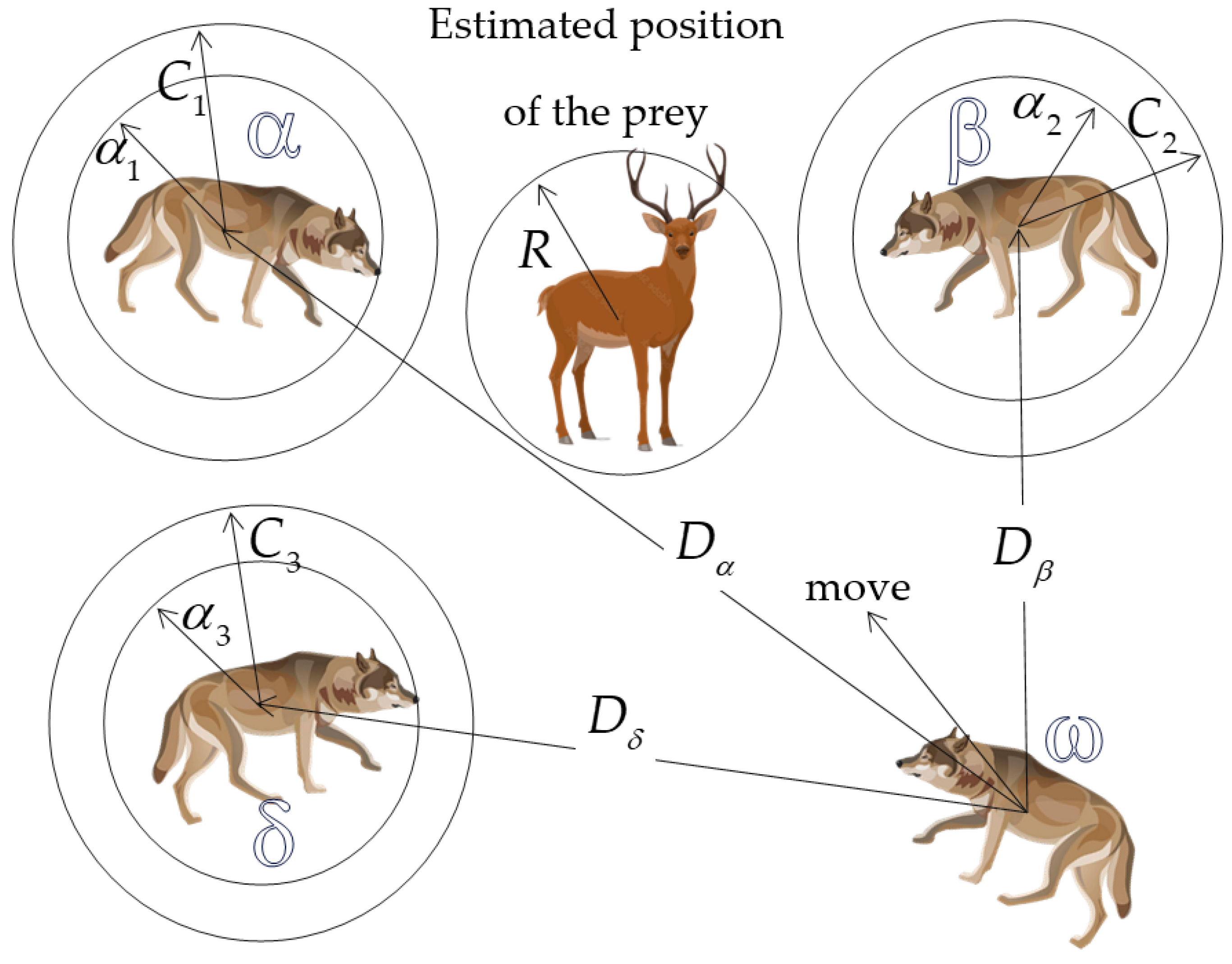
Wolf Ranking—The wolves are sorted based on their fitness levels. From this ranking, the top three wolves are identified. The fittest wolf is designated as the alpha (α), followed by the beta (β) as the second-fittest, and the delta (δ) as the third-fittest. All other wolves in the ranking after these three are considered omegas (ω).

Step 4:

Position Updating—Update the positions of the beta and delta wolves relative to the alpha wolf using Equation (35) for approaching and attacking. The omegas update their positions in relation to all three dominant wolves (alpha, beta, and delta), according to Equation (36).

Step 5:

Convergence Check—Calculate the fitness of all wolves using Equation (49), then update their positions. Check if a stopping criterion is met, such as a maximum number of iterations, a minimum error requirement, or another convergence indicator. If the stopping criterion is not satisfied, return to Step 2, and continue the iterations.

Step 6:

Solution Extraction—Once convergence is achieved or the stopping criterion is met, the alpha wolf’s position represents the optimal solution (or a near-optimal solution) to the problem.

6. Simulation Results and Discussion

The efficacy of the proposed approach was verified and then tested on standard IEEE 33-bus, 69-bus, and 85-bus test networks. The proposed I-GWO algorithm was coded in MATLAB 9.11 and executed on an Intel Core i7-8700K (3.7 GHz, 32 GB RAM) with Microsoft Windows 11 installed. As discussed earlier, the backward/forward sweep technique was employed for load flow calculations. The parameters utilized in the simulation for the three test systems can be found in

Table 2. Parameters in the I-GWO method.

Test System	33-Bus			69-Bus			85-Bus
Number of DSTATCOMs	Single	Two	Three	Single	Two	Three	Single	Two	Three
Population Size	100	200	400	200	500	800	400	800	1000
Max Iterations of I-GWO	500	1000	2000	500	1000	2000	500	1000	2000
$\overrightarrow{a}$ Range	[0, 2]	[0, 2]	[0, 2]	[0, 2]	[0, 2]	[0, 2]	[0, 2]	[0, 2]	[0, 2]
Max Iteration of Load Flow	50	50	50	50	50	50	50	50	50
Tolerance of Load Flow	10−5	10−5	10−5	10−5	10−5	10−5	10−5	10−5	10−5

.

Two scenarios were considered for each tested system for the optimal allocation and sizing of DSTATCOMs:

• Scenario (1): This scenario did not consider the presence of renewable generations and assumed a fixed load demand.
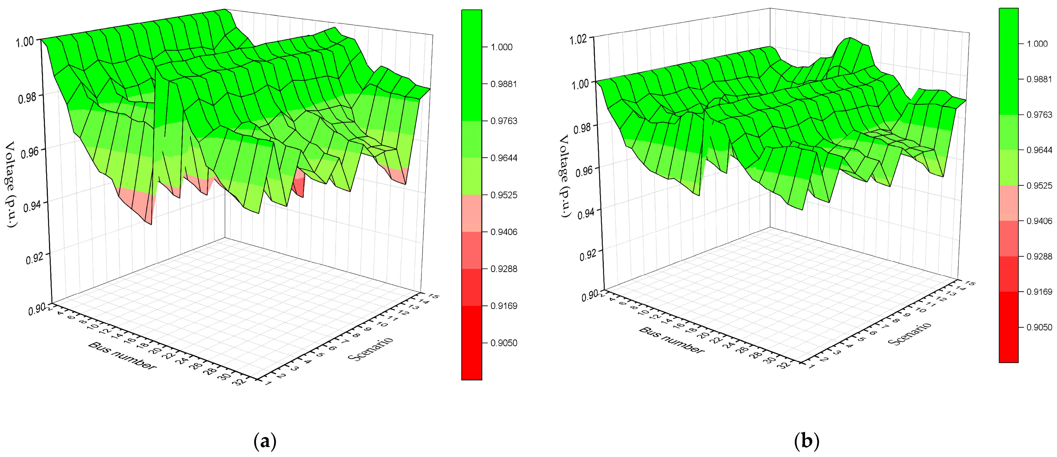
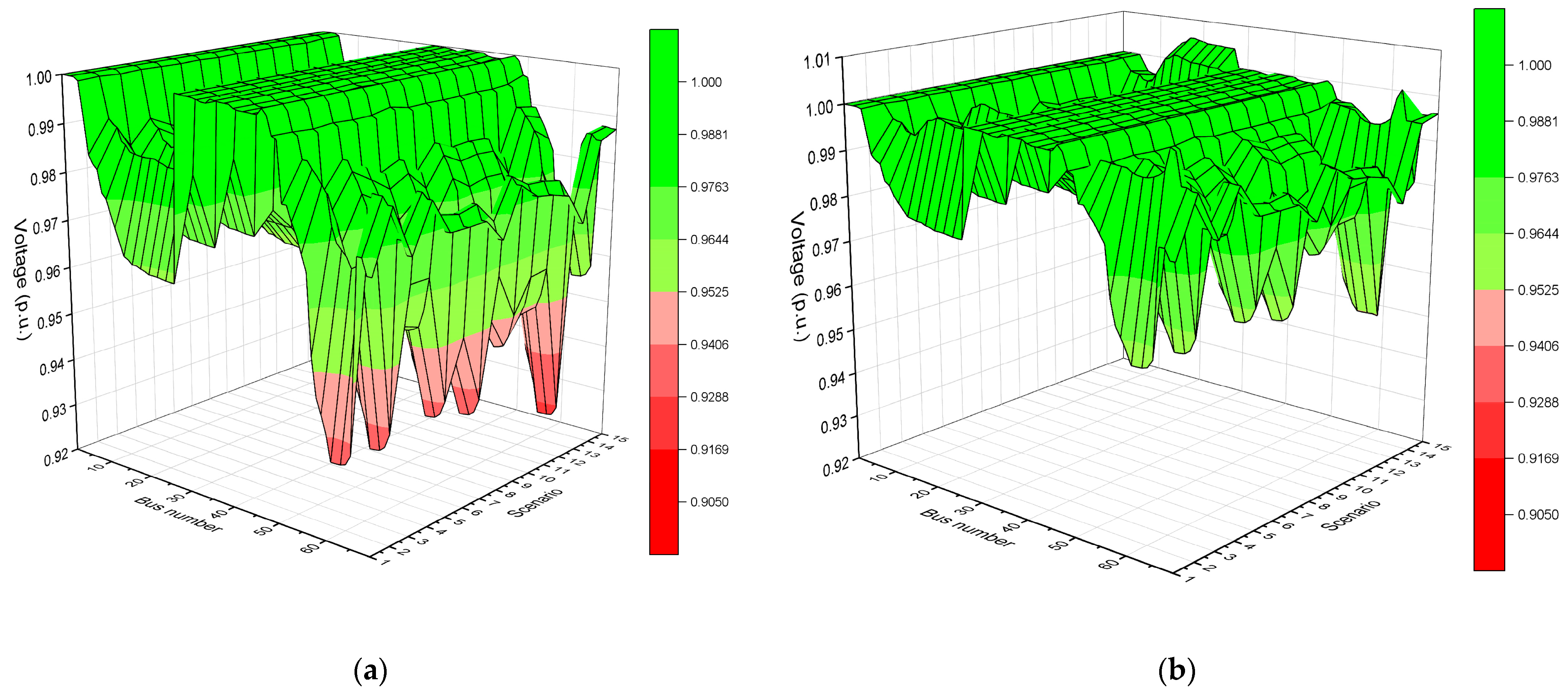
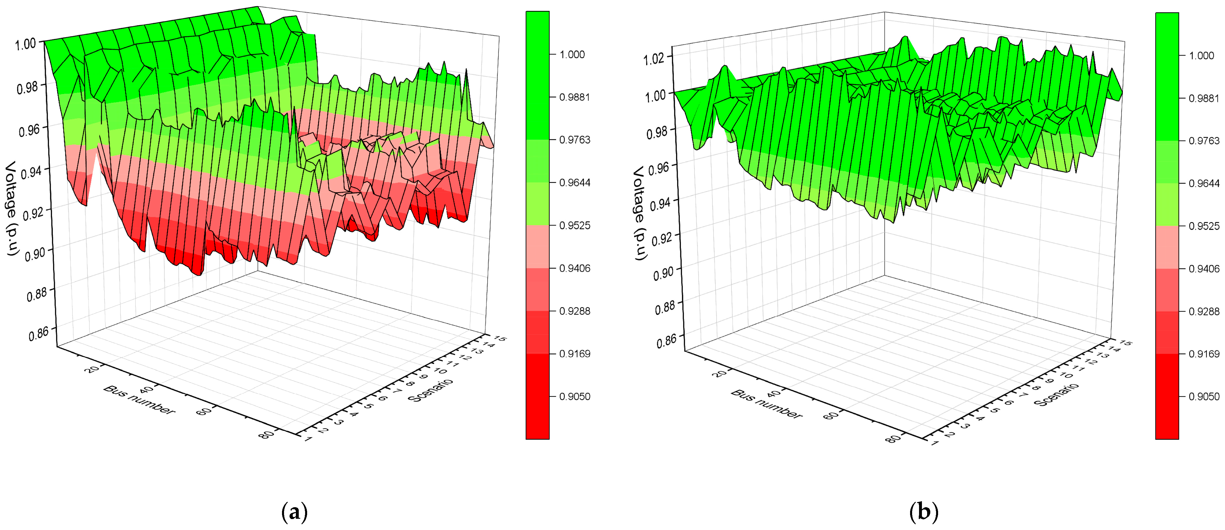
• Scenario (2): This scenario considered the presence of renewable energies located at predefined positions, also considering uncertain generation and load uncertainty.

6.1. Scenario (1)

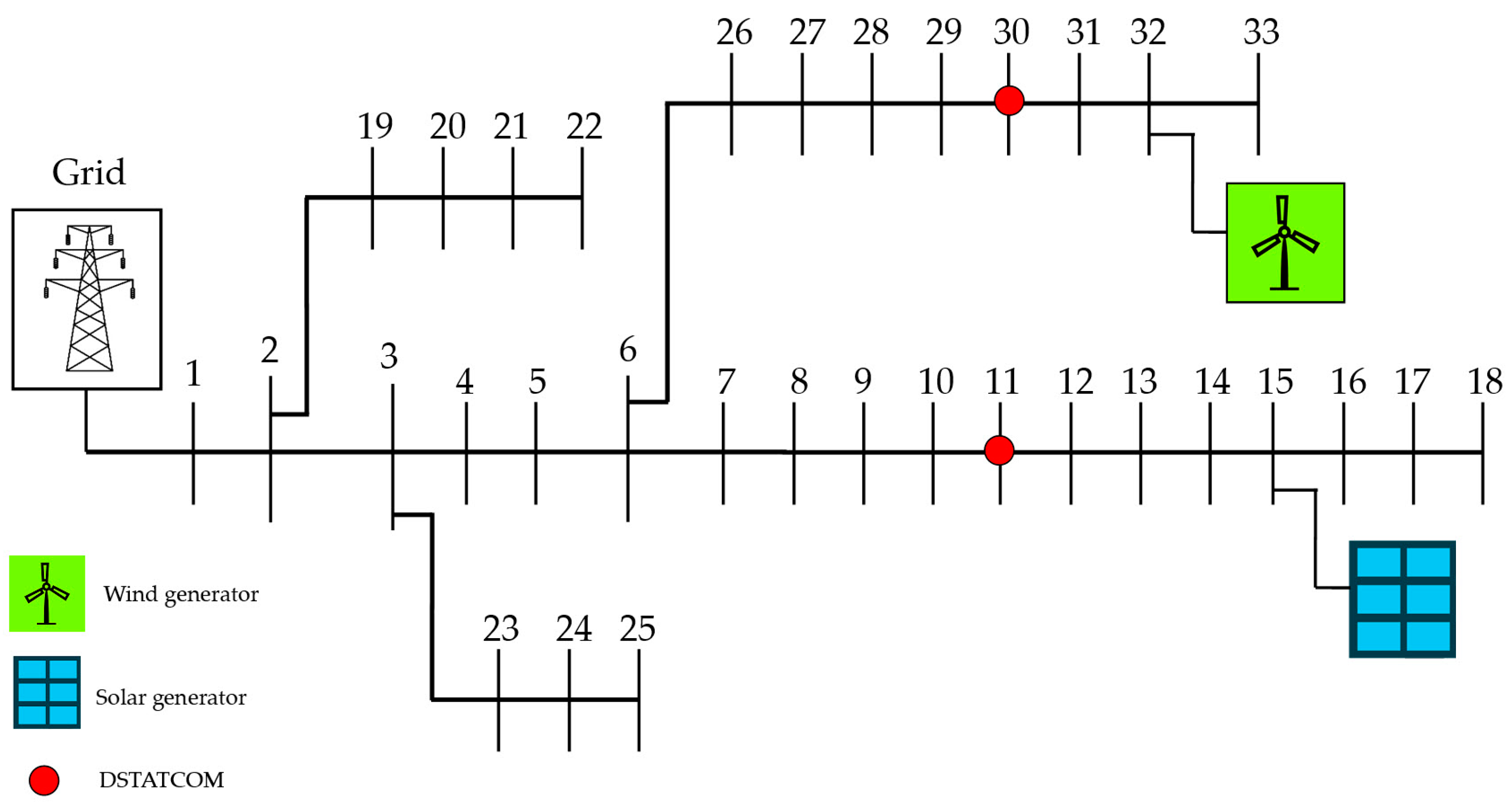
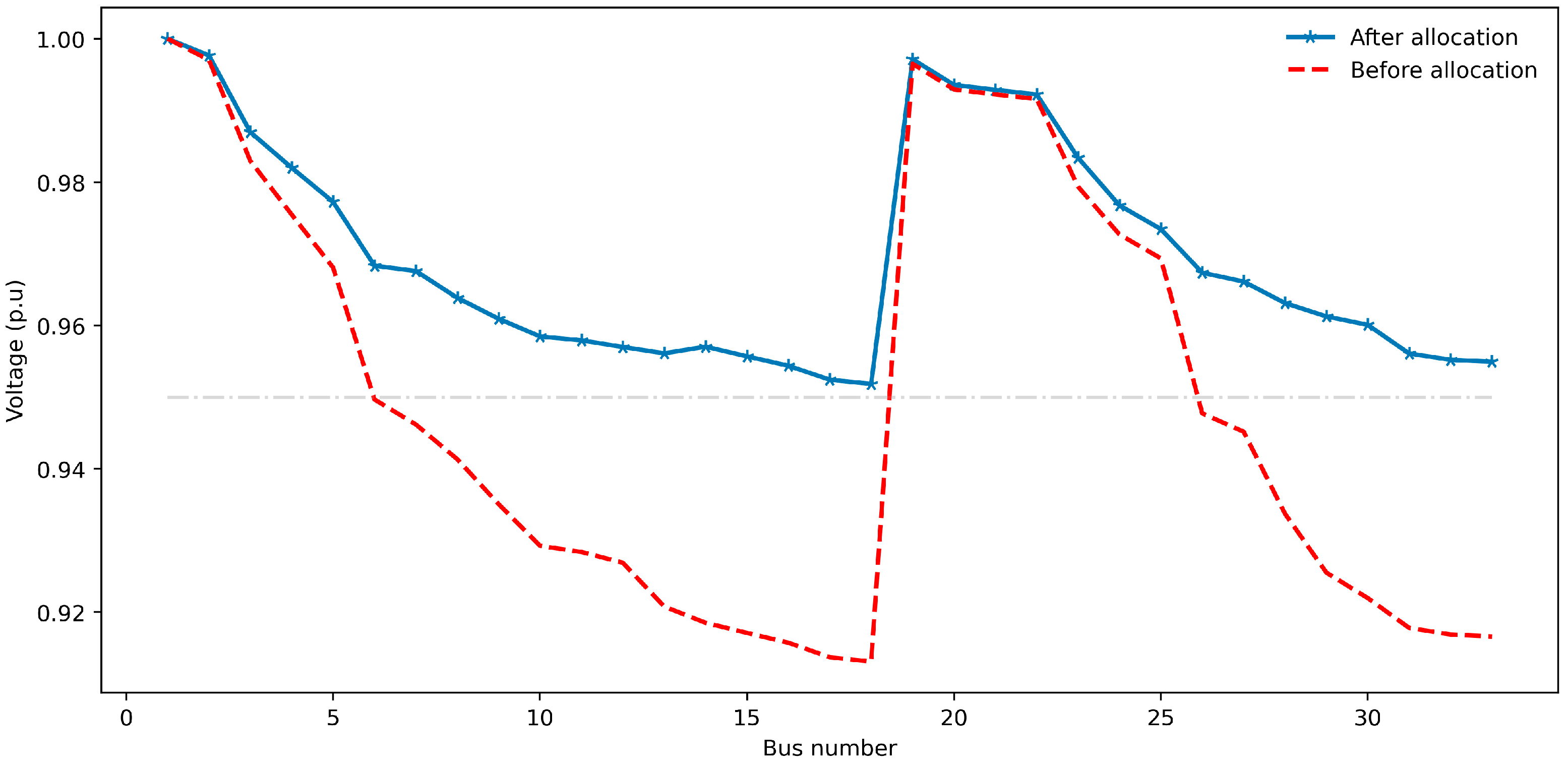
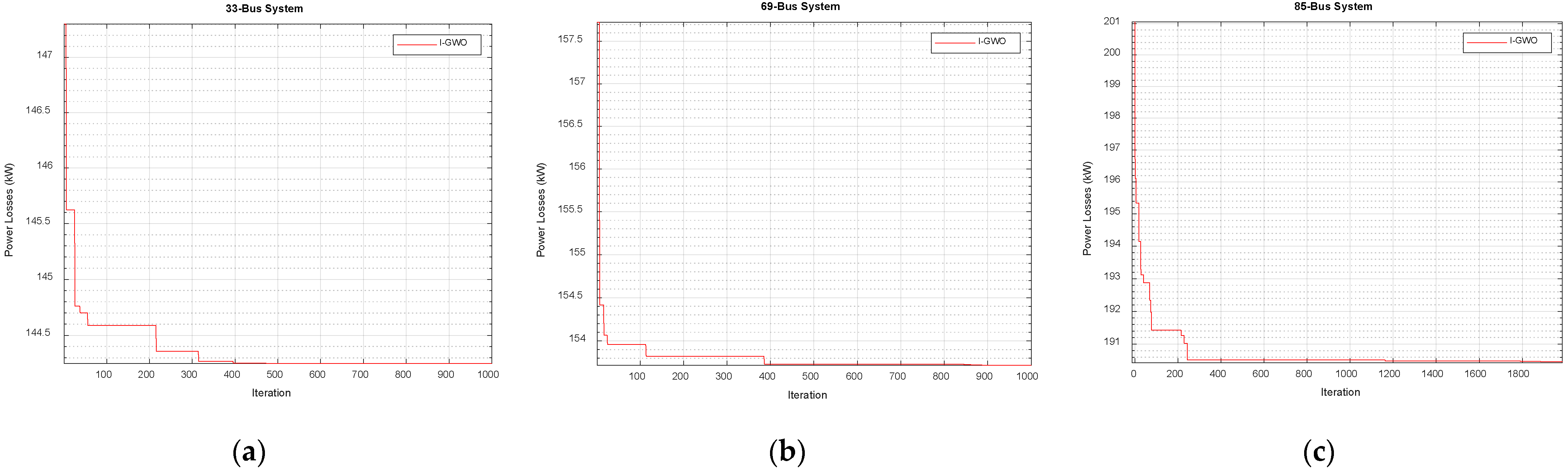
6.1.1. The 33-Bus Test System

The first tested network was a 33-bus radial distribution system with 33 buses and 32 branches [25]. It operated at a base voltage of 12.66 kV, with an apparent base power of 10 MVA. Without compensation, precisely without the DSTATCOM installation in the RDS, the active power loss was 202.68 kW, costing 106,526.61 USD/year. The minimum voltage and VSI values were 0.91309 and 0.69511 p.u., respectively. Detailed system data can be found in the Appendix A.

Table 3. Results for the IEEE 33-bus system.

Outputs	Base Case	Number of DSTATCOMs
		Single	Two	Three
Optimal size (kVAr) and location		1850.00 (30)	699.58 (14) 1386.89 (30)	953.38 (7) 477.22 (14) 1044.78 (30)
Ploss (kW)	202.68	153.27	144.23	141.31
% Reduction in Ploss		24.37	28.84	30.28
Vmin (p.u.)	0.91309	0.93031	0.95184	0.95324
VSImin (p.u.)	0.69511	0.74904	0.82083	0.82567
Cost of loss (USD/yr)	106,526.61	80,561.00	75,806.05	74,275.08
Cost of DSTATCOMs (USD/yr)		9812.33	11,066.52	13,129.36
TACS (USD/yr)		16,153.27	19,654.05	19,121.17

presents the optimization results for three cases: the insertion of single, two, and three DSTATCOMs. The optimal locations and sizes of the DSTATCOMs were determined using the I-GWO algorithm. The table shows that active power losses decreased in all three cases. Additionally, the minimum voltage increased, and the voltage stability index improved. The results show that the case with two DSTATCOMs offered the highest TACS compared to the other two cases. This suggests that there is an optimal number of DSTATCOM installations for the modeled distribution system that maximizes cost savings. Installing either fewer or more DSTATCOMs than this optimal number results in a diminished return on investment.

In the case of two DSTATCOMs, the proposed algorithm determined the optimal sizes to be 699.58 kVAr and 1386.89 kVAr. These were to be installed on buses 14 and 30, respectively. With this configuration, there was a total cost saving of USD 19,654.05 per year. Additionally, the total power losses were measured at 144.23 kW, equating to a significant reduction of 28.84% compared to the base case. It is also worth highlighting the improvement in the voltage profile of the test system, as illustrated in Figure 10. Specifically, the minimum voltage level was enhanced from 0.91309, as observed in the base case, to 0.95184 with the two DSTATCOMs in place, while the maximum voltage level remained at 1.0 p.u. at the source bus.

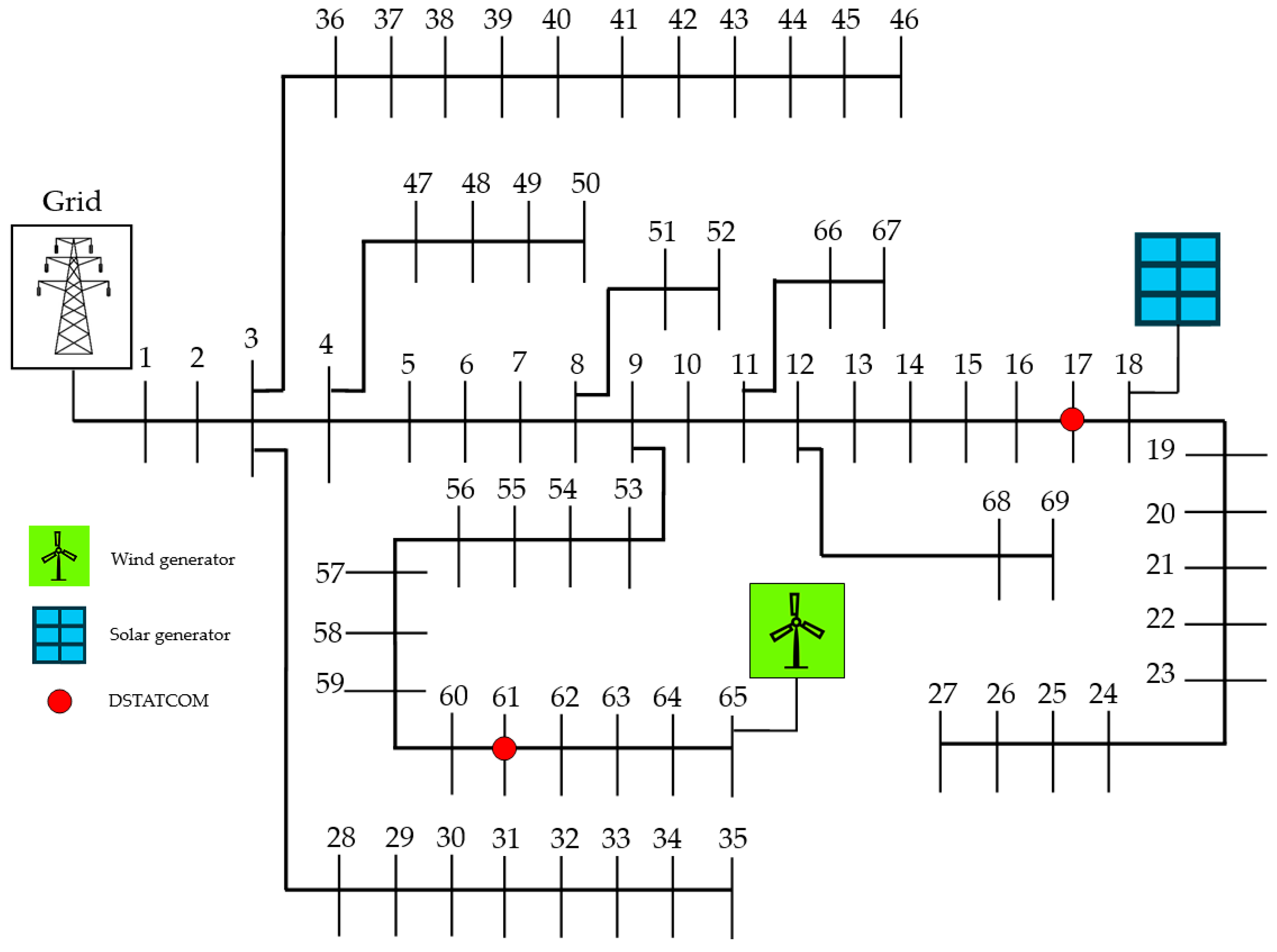
6.1.2. IEEE 69-Bus Test System

The efficacy of the I-GWO algorithm was further tested on a medium-scale radial distribution system, specifically, the IEEE 69-bus system [26]. The capacity base for this system was set at 1 MVA, while its voltage base was 12.66 kV. The data for the system were obtained from [27] and can be found in Appendix B. This test system carried a total load of 3.80 MW and 2.69 MVAR. The total losses amounted to 224.99 kW, which translated to an annual cost of 118,254.41 USD/year. Notably, the minimum voltage was observed to be 0.90919 p.u. at bus 65, and the maximum voltage was 1.0 p.u. at the source bus.

Table 4. Results for the IEEE 69-bus system.

Outputs	Base Case	Number of DSTATCOMs
		Single	Two	Three
Optimal size (kVAr) and location		1850 (61)	556.34 (17) 1474.55 (61)	820.24 (9) 500.03 (17) 1351.73 (61)
Ploss (kW)	224.99	158.49	153.73	154.12
% Reduction in Ploss		29.56	31.67	31.50
Vmin (p.u.)	0.90919	0.93665	0.95144	0.95219
VSImin (p.u.)	0.68331	0.76968	0.81947	0.82205
Cost of loss (USD/yr)	118,254.41	83,301.84	80,798.93	81,006.31
Cost of DSTATCOMs (USD/yr)		9812.33	10,771.76	14,172.17
TACS (USD/yr)		25,140.24	26,683.72	23,075.93

indicates that in the case with two DSTATCOMs installed, the TACS amounts to USD 26,683.72 per year, which is superior to the other cases. The minimum voltage increased to 0.95144 at bus 65, as observed in Figure 11. Additionally, power losses were reduced to 153.73 kW, representing a 31.67% reduction compared to the base case.

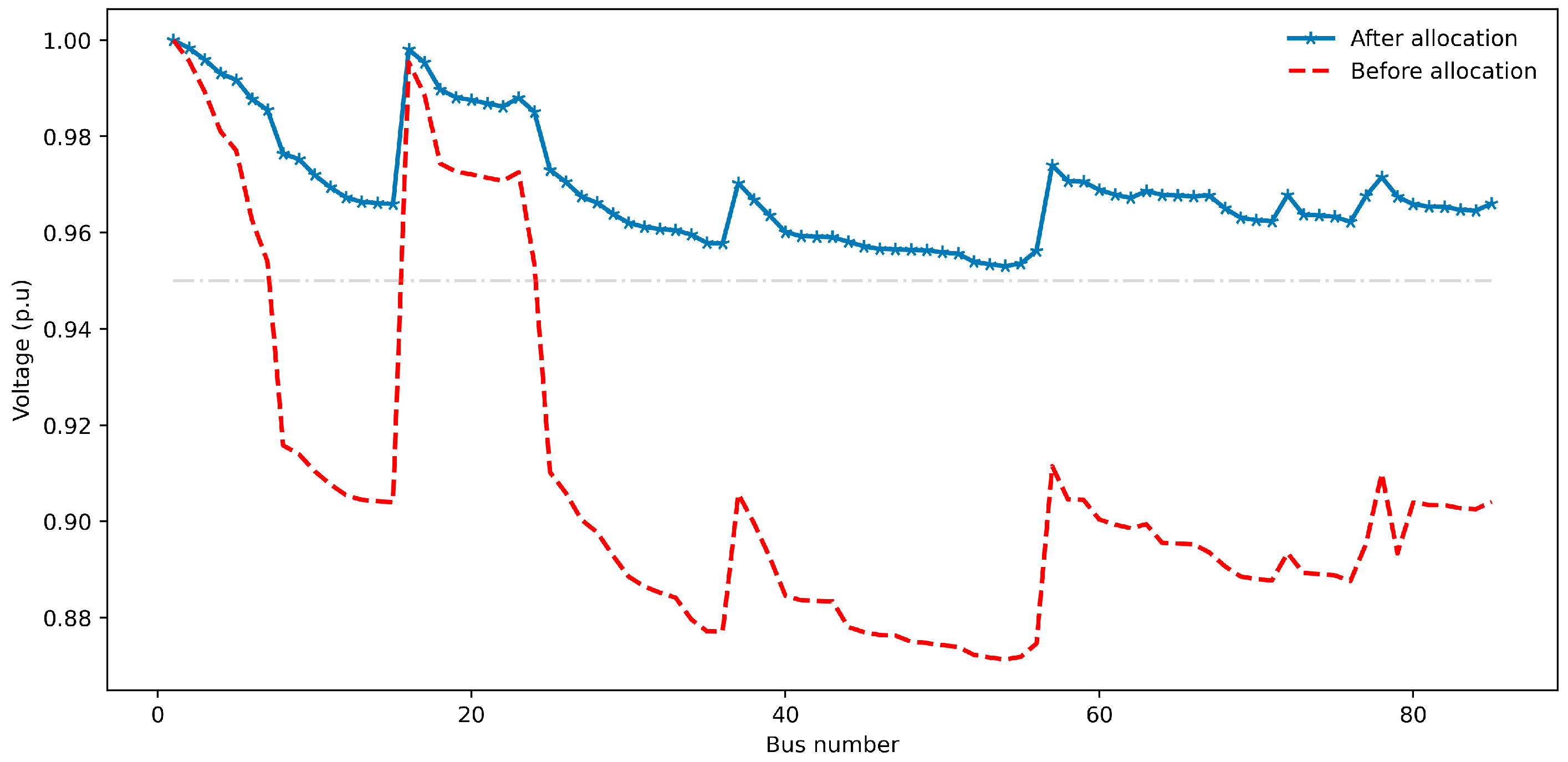
6.1.3. IEEE 85-Bus Test System

The 85-bus test case employed a radial distribution system consisting of a main feeder, four sub-feeders (laterals), and 13 sub-laterals. The data for the system were obtained from [27] and can be found in the Appendix C. The total load of the system was 2574.3 kW and 2622.6 kVAr.

For the 85-bus radial distribution system case, as detailed in

Table 5. Results for the IEEE 85-bus system.

Outputs	Base Case	Number of DSTATCOMs
		Single	Two	Three
Optimal size (kVAr) and location		2150 (32)	2150.00 (9) 1286.23 (32)	1929.15 (8) 896.70 (34) 727.25 (67)
Ploss (kW)	316.19	229.11	200.08	190.51
% Reduction in Ploss		32.12	36.72	39.75
Vmin (p.u.)	0.87129	0.93176	0.95219	0.95304
VSImin (p.u.)	0.57631	0.75373	0.82171	0.82499
Cost of loss (USD/yr)	166,189.63	120,419.81	105,163.24	100,131.51
Cost of DSTATCOMs (USD/yr)		11,403.52	18,225.65	18,845.46
TACS (USD/yr)		34,366.30	42,800.74	47,212.50

, installing three DSTATCOMs at buses 8, 34, and 67 resulted in the most cost-effective outcome, realizing an annual profit of USD 47,212.50. This optimal configuration substantially reduced the total losses to 190.51 kW, marking a decline of 39.75% compared to the base case. As illustrated in Figure 12, the voltage profile improved significantly, along with the economic advantages and loss reductions, with the minimum voltage level elevated to 0.95304 p.u., while maintaining the maximum voltage level of 1.0 p.u. at the source bus. The convergence behavior of the I-GWO algorithm for the three test systems is depicted in Figure 13.

6.2. Scenario (2)

In this scenario, the RES were located at predefined locations, and both generation and load were uncertain. Data for the RES and their locations for each study case are provided in the Appendices. In this paper, the scenario reduction process was applied using the FSR method, as discussed in the previous section, to reduce the number of wind and solar generation scenarios and loading levels to 15. Subsequently, the proposed I-GWO method was used to find the optimal location and sizing of the DSTATCOMs, considering all these 15 scenarios.

Table 6. Effects of DSTATCOMs in the presence of renewable generation and load uncertainty.

Outputs	33-Bus		69-Bus		85-Bus
	Without DSTATCOMs	With DSTATCOMs	Without DSTATCOMs	With DSTATCOMs	Without DSTATCOMs	With DSTATCOMs
Optimal size (kVAr) and location		696.15 (11) 1309.73 (30)		653.78 (17) 1459.28 (61)		1133.36 (9) 1073.75 (32) 468.16 (68)
Ploss (kW)	135.84	55.17	124.08	48.74	171.75	64.66
% Reduction in Ploss		59.39		58.18		62.35
Vmin (p.u.)	0.91109	0.95211	0.92155	0.95195	0.89245	0.95098
VSImin (p.u.)	0.68904	0.81178	0.72124	0.81493	0.63436	0.79202
Cost of loss (USD/yr)	71,396.33	48,123.80	65,214.82	32,567.67	90,271.13	37,289.27
Cost of DSTATCOMs (USD/yr)		10,639.09		11,207.57		14,189.55
TACS (USD/yr)		12,633.44		17,472.80		38,792.32

presents the main results obtained—such as power losses, minimum voltage, VSI, cost of loss, cost of DSTATCOMs, and TACS—for each study case, using the developed I-GWO method. For these cases, the number of DSTATCOMs selected was 2 for both the 33-bus and 69-bus test systems, and 3 for the 85-bus test system. Within Table 6, each study case is represented by two columns: the first column shows metrics before the installation of DSTATCOMs, and the second column displays metrics after their installation.

As illustrated, Table 6 reveals the significant impact of DSTATCOMs on reducing power losses across the IEEE 33-bus, 69-bus, and 85-bus systems. Specifically, for the 33-bus system, power losses were reduced from 135.84 to 55.17, achieving a reduction of 59.39% after installing 2 DSTATCOMs. The 69-bus system experienced a decrease in losses from 124.08 kW to 48.74 kW, translating to a 58.18% reduction with the installation of 2 DSTATCOMs. Lastly, the 85-bus system saw its power losses decline from 171.75 kW to 64.66 kW, amounting to a 62.35% reduction upon the integration of 3 DSTATCOMs. These reductions signify the pivotal role that DSTATCOMs play in enhancing the overall efficiency and reliability of radial distribution systems.

Figure 14, Figure 15 and Figure 16 present heatmaps that visualize voltage profiles for the three test systems, namely, 33-bus, 65-bus, and 85-bus, in the presence of renewable energies and load uncertainty. Before the installation of DSTATCOMs, these heatmaps partially display red areas that are indicative of low voltage levels below 0.95 p.u. Following the application of the proposed IGWO method for DSTATCOM sizing and placement, a noticeable shift to green can be observed in these figures. This color change signifies improved voltage levels, closer to 1 per unit, across all 15 scenarios. The transition clearly emphasizes the effectiveness of the optimal allocation and sizing of DSTATCOMs using the proposed IGWO method, in terms of improving voltage levels. The optimal locations for DSTATCOMs in the tree test systems are illustrated in the one-line diagrams found in Appendix D.

6.3. Comparative Analysis

The effectiveness of the proposed approach for the optimal sizing and allocation of DSTATCOMs in RDS is demonstrated through a comparison with other algorithms such as LSA [7], BFOA [9], CSA [10], MOSCA, and MOPSO, both from Reference [11]. All methodologies were assessed using the IEEE 33-bus and IEEE 69-bus systems based on installing three DSTATCOMs for a fair and consistent comparison. Notably, no method was identified in the literature reviewed that used the IEEE 85-bus test system. Each technique from the literature was aimed at the common objective of minimizing active power losses. It is important to mention that this comparison with these literature methods does not consider the presence of renewable generation sources and assumes a fixed load demand.

Table 7. Comparison of results with existing methods in the case of an IEEE 33-bus system.

Outputs	BFOA [9]	MOPSO [11]	LSA [7]	MOSCA [11]	Proposed Approach
Optimal size (kVAr) and location	632.00 (12) 487.00 (28) 550.00 (31)	679.21 (16) 549.50 (29) 722.03 (30)	341 (14) 516 (24) 1013 (30)	733.41 (8) 410.26 (16) 1029.04 (30)	400.72 (13) 554.87 (24) 1089.27 (30)
Ploss (kW)	144.38	152.44	138.35	150.27	132.16
Vmin (p.u.)	0.92400	0.95120	0.93010	0.9517	0.93774
VSImin (p.u.)	0.72280	0.81600	0.74230	0.81900	0.77327

and

Table 8. Comparison of the results with existing methods in the case of an IEEE 69-bus system.

Outputs	CSA [10]	MOPSO [11]	LSA [7]	MOSCA [11]	Proposed Approach
Optimal size (kVAr) and location	350.00 (25) 230.00 (18) 1170.00 (61)	906.40 (53) 846.50 (56) 1135.30 (62)	374.00 (11) 240.00 (18) 1217.00 (61)	226.60 (25) 1078.70 (62) 226.60 (63)	632.06 (9) 281.50 (19) 1149.94 (61)
Ploss (kW)	158.85	159.42	145.16	158.75	146.02
Vmin (p.u.)	0.93010	0.93660	0.93110	0.93890	0.92984
VSImin (p.u.)	0.74280	0.77120	0.74460	0.77700	0.74753

indicate that the proposed method outperforms the other techniques in terms of active power loss minimization, enhancement of voltage profiles, and voltage stability.

7. Conclusions

This study proposed the utilization of the improved gray wolf optimization (I-GWO) method to determine the optimal sizing and placement of DSTATCOMs in radial distribution systems. To address the limitations of the conventional gray wolf optimization (GWO) method, the I-GWO incorporated a dimension learning-based hunting (DLH) strategy. This strategy helped maintain population diversity, balance exploration and exploitation, and prevent premature convergence. The effectiveness of this optimization approach was verified through tests on the IEEE-33 bus, IEEE-69 bus, and 85-bus radial distribution systems. Furthermore, this method was compared to other prevalent optimization techniques, such as BFOA, CSA, LSA, MOPSO, and MOSCA. The proposed method, designed as an offline approach, demonstrated its superiority in terms of reducing active losses and costs. Moreover, it enhanced the voltage profile and stability and improved the quality of the entire system. In the second phase of this study, the model considered the uncertainties associated with renewable energy generation and load fluctuations. Initially, the fast scenario reduction (FSR) method condensed wind and solar generation scenarios and loading levels into a limited number of scenarios. Following this, the I-GWO algorithm determined the optimum location and sizing for the DSTATCOMs, accounting for all the scenarios identified by the FSR method, thereby demonstrating its effectiveness even under the conditions of renewable energy and load uncertainty across various test systems.

Further Research

While this study proposes I-GWO as an offline method, it shares common limitations with any metaheuristic, such as time consumption, especially in the case of large-scale distribution networks. Therefore, a potential avenue for future research lies in enhancing this approach or exploring hybridization with other optimization techniques to effectively address these limitations.

References

1. Mohammedi, R.D.; Mosbah, M.; Hellal, A.; Arif, S. An efficient BBO algorithm for optimal allocation and sizing of shunt capacitors in radial distribution networks. In Proceedings of the 2015 4th International Conference on Electrical Engineering (ICEE), Boumerdes, Algeria, 13–15 December 2015; pp. 1–5. [Google Scholar]
2. Mosbah, M.; Mohammedi, R.D.; Arif, S.; Hellal, A. Optimal of shunt capacitor placement and size in Algerian distribution network using particle swarm optimization. In Proceedings of the 2016 8th International Conference on Modelling, Identification and Control (ICMIC), Boumerdes, Algeria, 15–17 November 2016; pp. 192–197. [Google Scholar]
3. Jazebi, S.; Hosseinian, S.H.; Vahidi, B. DSTATCOM allocation in distribution networks considering reconfiguration using differential evolution algorithm. Energy Convers. Manag. 2011, 52, 2777–2783. [Google Scholar] [CrossRef]
4. Devi, S.; Geethanjali, M. Optimal location and sizing determination of Distributed Generation and DSTATCOM using Particle Swarm Optimization algorithm. Int. J. Electr. Power Energy Syst. 2014, 62, 562–570. [Google Scholar] [CrossRef]
5. Castiblanco-Pérez, C.M.; Toro-Rodríguez, D.E.; Montoya, O.D.; Giral-Ramírez, D.A. Optimal Placement and Sizing of D-STATCOM in Radial and Meshed Distribution Networks Using a Discrete-Continuous Version of the Genetic Algorithm. Electronics 2021, 10, 1452. [Google Scholar] [CrossRef]
6. Taher, S.A.; Afsari, S.A. Optimal location and sizing of DSTATCOM in distribution systems by immune algorithm. Int. J. Electr. Power Energy Syst. 2014, 60, 34–44. [Google Scholar] [CrossRef]
7. Thangaraj, Y.; Kuppan, R. Multi-objective simultaneous placement of DG and DSTATCOM using novel lightning search algorithm. J. Appl. Res. Technol. 2017, 15, 477–491. [Google Scholar] [CrossRef]
8. Yuvaraj, T.; Ravi, K.; Devabalaji, K.R. DSTATCOM allocation in distribution networks considering load variations using bat algorithm. Ain Shams Eng. J. 2017, 8, 391–403. [Google Scholar] [CrossRef]
9. Devabalaji, K.R.; Ravi, K. Optimal size and siting of multiple DG and DSTATCOM in radial distribution system using Bacterial Foraging Optimization Algorithm. Ain Shams Eng. J. 2016, 7, 959–971. [Google Scholar] [CrossRef]
10. Kaliaperumal Rukmani, D.; Thangaraj, Y.; Subramaniam, U.; Ramachandran, S.; Madurai Elavarasan, R.; Das, N.; Baringo, L.; Imran Abdul Rasheed, M. A New Approach to Optimal Location and Sizing of DSTATCOM in Radial Distribution Networks Using Bio-Inspired Cuckoo Search Algorithm. Energies 2020, 13, 4615. [Google Scholar] [CrossRef]
11. Selim, A.; Kamel, S.; Jurado, F. Optimal allocation of distribution static compensators using a developed multi-objective sine cosine approach. Comput. Electr. Eng. 2020, 85, 106671. [Google Scholar] [CrossRef]
12. Mirjalili, S.; Mirjalili, S.M.; Lewis, A. Grey Wolf Optimizer. Adv. Eng. Softw. 2014, 69, 46–61. [Google Scholar] [CrossRef]
13. Nadimi-Shahraki, M.H.; Taghian, S.; Mirjalili, S. An improved grey wolf optimizer for solving engineering problems. Expert Syst. Appl. 2021, 166, 113917. [Google Scholar] [CrossRef]
14. Dash, S.K.; Mishra, S.; Abdelaziz, A.Y. A Critical Analysis of Modeling Aspects of D-STATCOMs for Optimal Reactive Power Compensation in Power Distribution Networks. Energies 2022, 15, 6908. [Google Scholar] [CrossRef]
15. Chakravorty, M.; Das, D. Voltage stability analysis of radial distribution networks. Int. J. Electr. Power Energy Syst. 2001, 23, 129–135. [Google Scholar] [CrossRef]
16. Kawambwa, S.; Mwifunyi, R.; Mnyanghwalo, D.; Hamisi, N.; Kalinga, E.; Mvungi, N. An improved backward/forward sweep power flow method based on network tree depth for radial distribution systems. J. Electr. Syst. Inf. Technol. 2021, 8, 7. [Google Scholar] [CrossRef]
17. Hassan, M.H.; Kamel, S.; Hussien, A.G. Optimal power flow analysis considering renewable energy resources uncertainty based on an improved wild horse optimizer. IET Gener. Transm. Distrib. 2023, 17, 3582–3606. [Google Scholar] [CrossRef]
18. Ali, Z.M.; Diaaeldin, I.M.; HE Abdel Aleem, S.; El-Rafei, A.; Abdelaziz, A.Y.; Jurado, F. Scenario-Based Network Reconfiguration and Renewable Energy Resources Integration in Large-Scale Distribution Systems Considering Parameters Uncertainty. Mathematics 2021, 9, 26. [Google Scholar] [CrossRef]
19. Dupačová, J.; Gröwe-Kuska, N.; Römisch, W. Scenario reduction in stochastic programming. Math. Program. 2003, 95, 493–511. [Google Scholar] [CrossRef]
20. Mohammedi, R.D.; Mosbah, M.; Kouzou, A. Multi-Objective Optimal Scheduling for Adrar Power System including Wind Power Generation. Electroteh. Electron. Autom. 2018, 66, 102–109. [Google Scholar]
21. Mohammedi, R.D.; Zine, R.; Mosbah, M.; Arif, S. Optimum network reconfiguration using grey wolf optimizer. TELKOMNIKA (Telecommun. Comput. Electron. Control) 2018, 16, 2428–2435. [Google Scholar] [CrossRef]
22. Mirjalili, S. Improved Grey Wolf Optimizer (I-GWO). Available online: https://www.mathworks.com/matlabcentral/fileexchange/81253 (accessed on 22 August 2023).
23. Shahryari, E.; Shayeghi, H.; Moradzadeh, M. Probabilistic and Multi-Objective Placement of D-STATCOM in Distribution Systems Considering Load Uncertainty. Electr. Power Compon. Syst. 2018, 46, 27–42. [Google Scholar] [CrossRef]
24. Rahimi, I.; Gandomi, A.H.; Chen, F.; Mezura-Montes, E. A Review on Constraint Handling Techniques for Population-based Algorithms: From single-objective to multi-objective optimization. Arch. Comput. Methods Eng. 2023, 30, 2181–2209. [Google Scholar] [CrossRef]
25. Dolatabadi, S.H.; Ghorbanian, M.; Siano, P.; Hatziargyriou, N.D. An Enhanced IEEE 33 Bus Benchmark Test System for Distribution System Studies. IEEE Trans. Power Syst. 2021, 36, 2565–2572. [Google Scholar] [CrossRef]
26. Khodabakhshian, A.; Andishgar, M.H. Simultaneous placement and sizing of DGs and shunt capacitors in distribution systems by using IMDE algorithm. Int. J. Electr. Power Energy Syst. 2016, 82, 599–607. [Google Scholar] [CrossRef]
27. Prakash, D.B.; Lakshminarayana, C. Optimal siting of capacitors in radial distribution network using Whale Optimization Algorithm. Alex. Eng. J. 2017, 56, 499–509. [Google Scholar] [CrossRef]
Figure 1. Before installing DSTATCOM.
Applsci 14 00556 g001
Figure 2. After installing DSTATCOM.
Applsci 14 00556 g002
Figure 3. Vector representation of voltage and current phasors.
Applsci 14 00556 g003
Figure 4. Hourly wind speed over a year.
Applsci 14 00556 g004
Figure 5. Hourly solar irradiation over a year.
Applsci 14 00556 g005
Figure 6. Hourly loading level over a year.
Applsci 14 00556 g006
Figure 7. (a) Focused variations over a day regarding loading level; (b) focused variations over a day regarding wind speed and irradiation.
Applsci 14 00556 g007
Figure 8. Gray wolf hunting strategy.
Applsci 14 00556 g008
Figure 9. Structure of a wolf.
Applsci 14 00556 g009
Figure 10. Effect on voltage profile for the 33-bus system.
Applsci 14 00556 g010
Figure 11. Effect on voltage profile for the 69-bus system.
Applsci 14 00556 g011
Figure 12. Effect on voltage profile for the 85-bus system.
Applsci 14 00556 g012
Figure 13. (a) Convergence behavior for the IEEE 33-bus network; (b) convergence behavior for the IEEE 69-bus network; (c) convergence behavior for the IEEE 85-bus network.
Applsci 14 00556 g013
Figure 14. (a) Voltage profile for the IEEE 33-bus network without DSTATCOMs; (b) voltage profile for the IEEE 33-bus network with DSTATCOMs.
Applsci 14 00556 g014
Figure 15. (a) Voltage profile for the IEEE 69-bus network without DSTATCOMs; (b) voltage profile for the IEEE 69-bus network with DSTATCOMs.
Applsci 14 00556 g015
Figure 16. (a) Voltage profile for the IEEE 85-bus network without DSTATCOMs; (b) voltage profile for the IEEE 85-bus network with DSTATCOMs.
Applsci 14 00556 g016