Impedance-Based Stability Analysis of Grid-Connected Inverters under the Unbalanced Grid Condition

Abstract

As a common interface circuit for renewable energy integrated into the power grid, the inverter is prone to work under a three-phase unbalanced weak grid. In this paper, the instability of grid-connected inverters under the unbalanced grid condition is investigated. First, a dual second-order generalized integrator phase-locked loop (DSOGI-PLL)-based inverter under balanced and unbalanced conditions is modeled. A fourth-order impedance model is established to describe its impedance characteristics under the unbalanced grid condition. To analyze this multi-input multi-output system, a simplified stability analysis method based on the generalized Nyquist stability criterion and matrix theory is proposed. Then, the influences of circuit and control parameters on the stability of the grid-connected inverter system under the unbalanced grid condition are investigated. Finally, the accuracy of the derived frequency-coupled impedance model is verified via simulations, and the effectiveness of the proposed simplified stability analysis method on the system stability analysis is verified via both simulations and hardware experiments.

1. Introduction

In recent years, the penetration level of generated renewable energy such as wind and solar power into the power system has increased [1]. In grid-connected devices for renewable energy generation, inverters are widely applied [2,3,4]. Photovoltaic power stations and wind farms are usually located in remote places, and electricity generated by renewable energy sources needs to be transmitted over long distances [5]. For long-distance transmission lines, the line impedance and transformer impedance cannot be ignored, and various faults may occur throughout the line, which make the grid extremely sensitive to vulnerability and unbalance [6,7,8]. Due to the complex interaction between inverters and the weak and unbalanced power grid, there are many oscillation events caused by inverters in the power system [9,10]. Hence, the stability analysis of a grid-connected inverter system is significant for improving the utilization rate of renewable energy and maintaining the stable operation of the whole power system [11,12].

Stability analysis methods for inverter systems are mainly categorized into time-domain-based and frequency-domain-based analysis methods [13,14,15,16,17]. The state-space-model-based time-domain analysis method has been investigated for a long time and the techniques are very mature [13]. However, due to the large number of black-box and grey-box devices accessed by modern power systems, the time-domain approach is not valid or efficient [14]. Moreover, the topology of modern power systems is rapidly changing, leading to inefficient analysis using time-domain methods. In recent years, impedance-model-based frequency-domain analysis methods have attracted researchers and scholars due to their great advantages in modeling, measurement, and scalability [15]. Impedance models can be categorized into sequence impedance models and dq-axis impedance models [16,17]. Compared with the latter, the physical meaning of the sequence impedance model is clear and the sequence impedance model is highly scalable, so it is more suitable for modern power systems. Therefore, the sequence impedance-based modeling method and stability analysis method are adopted in this paper.

A weak and unbalanced grid condition will result in an inaccurate phase being obtained by the phase-locked loop (PLL), and further cause oscillations in the PLL-based grid-following inverter system [18,19]. In addition, it has been found in recent years that PLL-induced oscillations exhibit frequency-coupling characteristics. The frequencies of the oscillation harmonic components are mirror-coupled about the fundamental frequency [20]. In addition to the PLL, the grid impedance and other dq-axis control asymmetries have a great influence on frequency-coupling oscillations [21,22]. The traditional impedance models consider the inverter as a single-input single-output (SISO) system with positive and negative sequence impedance decoupling. Obviously, the traditional impedance model cannot accurately describe the frequency coupling characteristics of the inverter. Frequency-coupled impedance modeling is significant for analyzing PLL-based grid-following inverters. Using the multi-harmonic linearization method, a detailed frequency-coupled impedance model of the voltage source converter has been established [23]. Various frequency-coupling factors such as PLL, outer DC voltage loop, and inner current loop are considered in [23].

The PLL is the most significant factor in the frequency-coupling effect. Many investigations have improved the implementation and structure of the PLL to achieve suppression of the frequency-coupling effect and enhance system stability [24,25,26]. Compared with the traditional synchronous reference frame phase-locked loop (SRF-PLL) and its improvement, the dual second-order generalized integrator PLL (DSOGI-PLL) is widely used under the grid condition where three-phase unbalance and complex system harmonics exist. The reason for this is that the DSOGI-PLL can accurately obtain the phase in the presence of three-phase unbalance and complex system harmonics [27]. However, the second-order generalized integrator (SOGI) of DSOGI-PLL cannot attenuate the low-frequency signal sufficiently, which can lead to low-frequency oscillations. Accurate small-signal models with frequency-adaptive DSOGI-PLL have been developed for DSOGI-PLL as well as PR current-controlled inverters [28]. However, studies on the stability of the inverter system under unbalanced grids, where DSOGI-PLL is most commonly used, are still lacking. Therefore, in this paper, the stability of DSOGI-PLL-based grid-connected inverter systems under a weak and unbalanced grid, on which few studies have been carried out until now, is investigated based on the impedance-based method.

There have been many studies on the influence of the unbalanced grid impedance on the stability of grid-connected inverters [29,30,31,32,33,34,35]. The multi-input multi-output (MIMO) impedance model has been established for inverters under the unbalanced grid condition. Therefore, to simplify the stability analysis steps, the individual channel method [32] is adopted to extract the SISO subsystems from the established MIMO models [33]. Similarly, the MIMO system is decomposed into three SISO systems [34]. However, these studies neglect the frequency-coupling effect, which may lead to inaccurate analysis results. Therefore, for the inverter working under the unbalanced grid condition, the coupling of sequence impedance caused by both the unbalance and the frequency-coupling effect should be considered for modeling. In [35], the impedance model of the inverter is established by considering the frequency-coupling effect and the unbalance through the harmonic transfer matrix-based method. And it is pointed out in [35] that the fourth-order impedance model can accurately describe the impedance characteristics of the inverter under the unbalanced grid condition. Inspired by this study, for investigating the DSOGI-PLL-based inverter under the unbalanced grid condition, a fourth-order impedance model considering the modeling of DSOGI-PLL is required to be established.

In summary, although there are many studies on the modeling and stability of inverters under unbalanced grid conditions, the modeling and stability analysis of DSOGI-PLL-based inverters under three-phase unbalanced conditions are not well developed. In order to remedy this deficiency, some investigations of the DSOGI-PLL-based inverter are carried out in this paper. For the stability analysis of higher-order MIMO systems, there are two common methods. One is to use the generalized Nyquist criterion (GNC) directly [29,30]. The other is to transform the frequency-coupled impedance model into equivalent decoupled sequence impedances via matrix diagonalization, and then use the SISO stability criterion [35]. However, for the stability analysis of a fourth-order system, this diagonalization method is very complicated and not suitable. And there may be RHP poles in the equivalent decoupled sequence impedance model, which will lead to incorrect stability analysis results [36]. Therefore, in this paper, based on the GNC and matrix theory, a simplified stability analysis method is proposed.

The main contributions of this paper are as follows

(1)

The frequency-coupled impedance models of the DSOGI-PLL-based inverter under the balanced and unbalanced grid conditions are derived. This provides the theoretical basis for the analysis of the impedance characteristics and stability of the DSOGI-PLL-based inverter.

(2)

Based on the GNC and matrix theory, the stability analysis of high-order systems is transformed into the analysis of eigenvalues of two second-order matrices, which simplifies the stability analysis process of high-order systems.

(3)

The influences of pivotal parameters on the stability of the DSOGI-PLL-based grid-connected inverter system are comprehensively investigated. The analysis results provide the theoretical basis for the parameter design of the DSOGI-PLL-based inverter.

In this paper, the methodology is illustrated in Figure 1. As shown in Figure 1, we first derive the frequency-coupled impedance model of the inverter based on the multi-harmonic linearization method and symmetric component method. Then, to verify the accuracy of the derived impedance model of the inverter, we establish a time-domain simulation model in the MATLAB/Simulink R2023a platform and carried out a frequency sweeping simulation. In Section 3, we propose a simplified stability analysis method based on the GNC and matrix theory to analyze the stability of higher-order systems. We establish the time-domain simulation model and hardware experimental platform to validate the effectiveness of the proposed analysis method. In Section 4, we analyze the influence of pivotal parameters on the system’s stability and discuss the parameter design recommendations for practical engineering. Based on the methodology shown in Figure 1, the low-frequency oscillations in the DSOGI-PLL-based inverter under the unbalanced grid condition are investigated. The main conclusions are drawn in Section 5.

2. Impedance Modeling of the DSOGI-PLL-Based Inverter and Verification

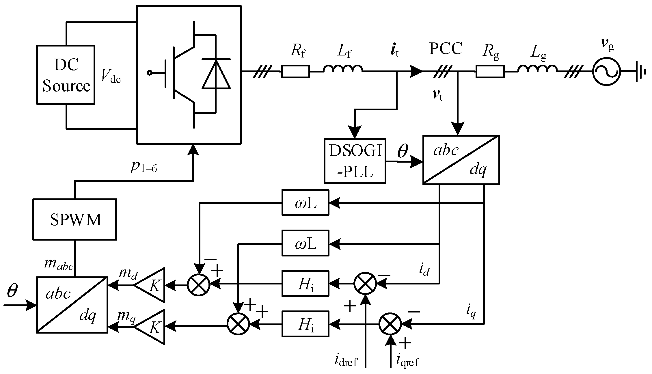
2.1. The Structure of the DSOGI-PLL-Based Grid-Connected Inverter

Figure 2 shows the structure of the DSOGI-PLL-based grid-connected inverter system. In the control system, i_d, i_dref, i_q, and i_qref represent the dq-axis sampled current and current reference at the PCC, respectively. m_dq and m_abc represent the dq- and abc-axis modulation signals, respectively. p_1–6 represents the switching signals. The single closed-loop control strategy is adopted in the control system, where H_i represents the PI controller.

For the power circuit, the AC side is connected to the grid through an L-type filter, and the DC side is connected to a constant voltage source to simplify the analysis. V_g and V_dc represent the grid voltage and DC-side voltage, respectively. R_g and L_g represent the resistance and inductance of the grid impedance, respectively. v_t and i_t represent the three-phase voltage and current at the point of common coupling (PCC), respectively.

The control structures of the SOGI and the DSOGI-PLL are shown in Figure 3, where v represents the input voltage signal; ε and k represent the error signal and damping coefficient, respectively; ω represents the resonance frequency; v′ and qv′ represent two orthogonal output signals, respectively; v_pα′, qv_pα′, v_pβ′, and qv_pβ′ represent the α- and β-axis components of the voltage signals processed by the SOGI, respectively; v_pα+ and v_pβ+ represent the α- and β-axis positive sequence components, respectively; v_pd+ and v_pq+ represent the d- and q-axis positive sequence components, respectively; k_p and k_i represent the proportional gain and integral gain of the PI controller in the PLL, respectively; and θ represents the output angle of the PLL.

2.2. Impedance Modeling under the Three-Phase Balanced Condition

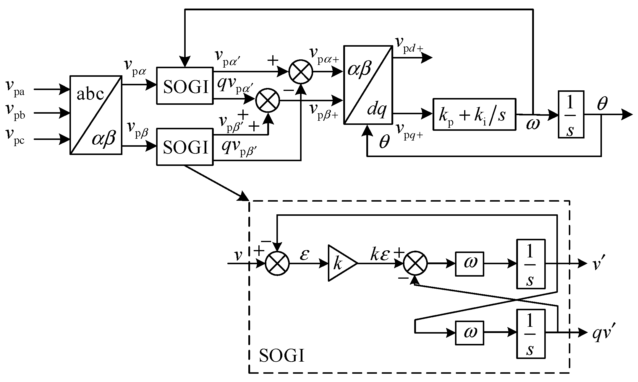
The frequency-coupled impedance model of the DSOGI-PLL-based grid-connected inverter is derived in this subsection. In the time domain, the a-phase voltage at the PCC is (taking the a-phase as an example, the other two phases lag the a-phase by 120° and 240°, respectively)

$$v_{\mathrm{ta}}(t)=V_1\cos ({\omega }_{1}t+{\phi }_{\mathrm{ta}})$$

(1)

where v_ta represents the a-phase voltage, V₁ represents the amplitude of the fundamental voltage, ω₁ = 2πf₁ represents the fundamental angular frequency, and φ_ta represents the initial phase of the a-phase voltage.

For the DSOGI-PLL-based grid-connected inverter system, the small-signal harmonic voltage is injected into the PCC as the perturbation. Therefore, the terminal voltage and output current at the PCC are

$${\mathit{V}}_{\mathrm{ta}}[f]=\left\{\begin{array}{l}{\mathit{V}}_1,f=f_1\\ {\mathit{V}}_{\mathrm{p}},f=f_{\mathrm{p}}\\ {\mathit{V}}_{\mathrm{c}},f=f_{\mathrm{c}}\end{array}\right.$$

(2)

$${\mathit{I}}_{\mathrm{ta}}[f]=\left\{\begin{array}{l}{\mathit{I}}_1,f=f_1\\ {\mathit{I}}_{\mathrm{p}},f=f_{\mathrm{p}}\\ {\mathit{I}}_{\mathrm{c}},f=f_{\mathrm{c}}\end{array}\right.$$

(3)

where V₁ and I₁ represent the voltage and current at the fundamental frequency, respectively. V_p and I_p represent the perturbation voltage and current, respectively. V_c and I_c represent the coupled voltage and current, respectively. f_p and f_c represent the coupled perturbation frequencies, f_p + f_c = 2f₁.

2.2.1. DSOGI-PLL

The phase of voltage at the PCC is obtained by the PLL, which is used as the phase reference of the control system. The modeling of the PLL is vital to analyzing the interaction stability between the inverter and the grid, so the small-signal model of the PLL should be first derived.

When the perturbation is applied to the system, there is a deviation in the output angle of the PLL. The output phase of the PLL can be expressed as

$$\theta ={\omega }_{1}t+\mathsf{\Delta }\theta$$

(4)

where θ is the output angle of the PLL, ω₁ is the fundamental angular frequency, and Δθ is the phase deviation.

The control block diagram of the SOGI is shown in Figure 3. The dq-axis positive-sequence signals (high-order small-signal components have been ignored) are expressed as

$${\mathit{V}}_{\mathrm{p}d+}=G_{\alpha 1}\left(s_1\right){\mathit{V}}_1+G_{\alpha \mathrm{p}}(s_{\mathrm{p}}-s_1){\mathit{V}}_{\mathrm{p}}+G_{\alpha \mathrm{c}}(s_1-s_{\mathrm{c}}){\mathit{V}}_{\mathrm{c}}$$

(5)

$${\mathit{V}}_{\mathrm{p}q+}=-\mathsf{\Delta }\mathit{\theta }\left[G_{\alpha 1}\left(s_1\right){\mathit{V}}_1+G_{\alpha \mathrm{p}}(s_{\mathrm{p}}-s_1){\mathit{V}}_{\mathrm{p}}+G_{\alpha \mathrm{c}}(s_1-s_{\mathrm{c}}){\mathit{V}}_{\mathrm{c}}\right]$$

(6)

where $G_{\alpha k}=G(s_k)+\mathrm{j}{G}_q(s_k)$, $G_{\beta k}=G_q(s_k)-\mathrm{j}G(s_k)$, $s_k=\mathrm{j}2\pi f_k$, and $k=1,\mathrm{p},\mathrm{c}$. And the transfer functions between two orthogonal output signals and the input signal are $G\left(s\right)=\frac{k{\omega }_{1}s}{s^2+k{\omega }_{1}s+{\omega }_1{}^2}$ and $G_q\left(s\right)=\frac{k{\omega }_1{}^2}{s^2+k{\omega }_{1}s+{\omega }_1{}^2}$.

According to the control structure of the PLL and Equations (6)–(11), the output angle of the DSOGI-PLL can be obtained

$$\mathsf{\Delta }\mathit{\theta }=T_{\mathrm{p}}\left(s\right){\mathit{V}}_{\mathrm{p}}+T_{\mathrm{c}}^{*}\left(s\right){\mathit{V}}_{\mathrm{c}}^{*}$$

(7)

where $T_{\mathrm{p}}(s)=\frac{-\mathrm{j}{H}_{\mathrm{pll}}\left(s-s_1\right)\left[G\left(s\right)+\mathrm{j}{G}_q\left(s\right)\right]}{1+\left[G_1\left(s\right)+\mathrm{j}{G}_{1q}\left(s\right)\right]{\mathit{V}}_1{H}_{\mathrm{pll}}\left(s-s_1\right)}$, $H_{\mathrm{pll}}\left(s-s_1\right)=\frac{k_{\mathrm{p}}+k_{\mathrm{i}}/\left(s-s_1\right)}{s-s_1}$, $T_{\mathrm{c}}^{*}\left(s\right)=\frac{\mathrm{j}{H}_{\mathrm{pll}}\left(s_1-s\right)\left[G\left(s_{\mathrm{c}}\right)+\mathrm{j}{G}_q\left(s_{\mathrm{c}}\right)\right]}{1+\left[G_1\left(s\right)+\mathrm{j}{G}_{1q}\left(s\right)\right]{\mathit{V}}_1{H}_{\mathrm{pll}}\left(s_1-s\right)}$, $H_{\mathrm{pll}}\left(s_1-s\right)=\frac{k_{\mathrm{p}}+k_{\mathrm{i}}/\left(s_1-s\right)}{s_1-s}$.

2.2.2. Park Transformation

Affected by the phase deviation, the dq-axis voltage and current after Park transformation will contain multiple harmonic components. The d- and q-axis current increments are

$${\mathit{I}}_d=G_{\mathrm{Id}-\mathrm{Vp}}{\mathit{V}}_{\mathrm{p}}+G_{\mathrm{Id}-\mathrm{Vc}}{\mathit{V}}_{\mathrm{c}}^{*}+{\mathit{I}}_{\mathrm{p}}+{\mathit{I}}_{\mathrm{c}}^{*}$$

(8)

$${\mathit{I}}_q=G_{\mathrm{Iq}-\mathrm{Vp}}{\mathit{V}}_{\mathrm{p}}+G_{\mathrm{Iq}-\mathrm{Vc}}{\mathit{V}}_{\mathrm{c}}^{*}+G_{\mathrm{Iq}-\mathrm{Ip}}{\mathit{I}}_{\mathrm{p}}+G_{\mathrm{Iq}-\mathrm{Ic}}{\mathit{I}}_{\mathrm{c}}^{*}$$

(9)

where $G_{\mathrm{Id}-\mathrm{Vp}}=I_1\sin {\phi }_{\mathrm{i}1}{T}_{\mathrm{p}}\left(s\right)$, $G_{\mathrm{Id}-\mathrm{Vc}}=I_1\sin {\phi }_{\mathrm{i}1}{T}_{\mathrm{c}}^{*}\left(s\right)$, $G_{\mathit{I}\mathrm{q}-\mathrm{Vp}}=-I_1\cos {\phi }_{\mathrm{i}1}{T}_{\mathrm{p}}\left(s\right)$, $G_{\mathrm{Iq}-\mathrm{Vc}}=-I_1\cos {\phi }_{\mathrm{i}1}{T}_{\mathrm{c}}^{*}\left(s\right)$, $G_{\mathrm{Iq}-\mathrm{Ip}}=-\mathrm{j}$, and $G_{\mathrm{Iq}-\mathrm{Ic}}=\mathrm{j}$. ${\phi }_{\mathrm{i}1}$ represents the phase angle of the current at the fundamental frequency.

2.2.3. Inner Current Loop

The modulation signals are obtained through the inner current loop, when the d- or q-axis current is perturbed, the dq-axis modulation signals will also contain multiple harmonic components. The d- and q-axis modulation signal increments are

$${\mathit{m}}_d=G_{\mathrm{md}-\mathrm{Vp}}{\mathit{V}}_{\mathrm{p}}+G_{\mathrm{md}-\mathrm{Ip}}{\mathit{I}}_{\mathrm{p}}+G_{\mathrm{md}-\mathrm{Vc}}{\mathit{V}}_{\mathrm{c}}^{*}+G_{\mathrm{md}-\mathrm{Ic}}{\mathit{I}}_{\mathrm{c}}^{*}$$

(10)

$${\mathit{m}}_q=G_{\mathrm{mq}-\mathrm{Vp}}{\mathit{V}}_{\mathrm{p}}+G_{\mathrm{mq}-\mathrm{Ip}}{\mathit{I}}_{\mathrm{p}}+G_{\mathrm{mq}-\mathrm{Vc}}{\mathit{V}}_{\mathrm{c}}^{*}+G_{\mathrm{mq}-\mathrm{Ic}}{\mathit{I}}_{\mathrm{c}}^{*}$$

(11)

where $G_{\mathrm{md}-\mathrm{Vp}}=\left(-H_{\mathrm{i}}{T}_{\mathrm{p}}{I}_1\sin {\phi }_{\mathrm{i}1}+\omega L{T}_{\mathrm{p}}{I}_1\cos {\phi }_{\mathrm{i}1}\right)/\left(V_{\mathrm{dc}}/2\right)$, $G_{\mathrm{md}-\mathrm{Ip}}=\left(-H_{\mathrm{i}}+\mathrm{j}\omega L\right)/\left(V_{\mathrm{dc}}/2\right)$, $G_{\mathrm{md}-\mathrm{Vc}}=\left(-H_{\mathrm{i}}{T}_{\mathrm{c}}^{*}{I}_1\sin {\phi }_{\mathrm{i}1}+\omega L{T}_{\mathrm{c}}^{*}{I}_1\cos {\phi }_{\mathrm{i}1}\right)/\left(V_{\mathrm{dc}}/2\right)$, $G_{\mathrm{md}-\mathrm{Ic}}=\left(-H_{\mathrm{i}}-\mathrm{j}\omega L\right)/\left(V_{\mathrm{dc}}/2\right)$, $G_{\mathrm{mq}-\mathrm{Vp}}=\left(\omega L{T}_{\mathrm{p}}{I}_1\sin {\phi }_{\mathrm{i}1}+H_{\mathrm{i}}{T}_{\mathrm{p}}{I}_1\cos {\phi }_{\mathrm{i}1}\right)/\left(V_{\mathrm{dc}}/2\right)$, $G_{\mathrm{mq}-\mathrm{Ip}}=\left(\omega L+\mathrm{j}{H}_{\mathrm{i}}\right)/\left(V_{\mathrm{dc}}/2\right)$, $G_{\mathrm{mq}-\mathrm{Vc}}=\left(\omega L{T}_{\mathrm{c}}^{*}{I}_1\sin {\phi }_{\mathrm{i}1}+H_{\mathrm{i}}{T}_{\mathrm{c}}^{*}{I}_1\cos {\phi }_{\mathrm{i}1}\right)/\left(V_{\mathrm{dc}}/2\right)$, and $G_{\mathrm{mq}-\mathrm{Ic}}=\left(\omega L-\mathrm{j}{H}_{\mathrm{i}}\right)/\left(V_{\mathrm{dc}}/2\right)$.

2.2.4. Inverse Park Transformation

The function of the inverse Park transformation is to transform modulation signals from the dq-axis to the abc-axis. The phasor expressions of the a-phase modulation signal increments in the frequency domain are

$${\mathit{m}}_a=\left\{\begin{array}{l}{G}_{\mathrm{ma}-\mathrm{Vp}}{\mathit{V}}_{\mathrm{p}}+G_{\mathrm{ma}-\mathrm{Vc}}{\mathit{V}}_{\mathrm{c}}^{*}+G_{\mathrm{ma}-\mathrm{Ip}}{\mathit{I}}_{\mathrm{p}}+G_{\mathrm{ma}-\mathrm{Ic}}{\mathit{I}}_{\mathrm{c}}^{*},f=f_{\mathrm{p}}\\ G_{\mathrm{mc}-\mathrm{Vp}}{\mathit{V}}_{\mathrm{p}}+G_{\mathrm{mc}-\mathrm{Vc}}{\mathit{V}}_{\mathrm{c}}^{*}+G_{\mathrm{mc}-\mathrm{Ip}}{\mathit{I}}_{\mathrm{p}}+G_{\mathrm{mc}-\mathrm{Ic}}{\mathit{I}}_{\mathrm{c}}^{*},f=f_{\mathrm{c}}\end{array}\right.$$

(12)

where $G_{\mathrm{ma}-\mathrm{Vp}}=0.5\mathrm{j}{M}_d{T}_{\mathrm{p}}+0.5G_{\mathrm{md}-\mathrm{Vp}}-0.5M_q{T}_{\mathrm{p}}+0.5\mathrm{j}{G}_{\mathrm{mq}-\mathrm{Vp}}$, $G_{\mathrm{ma}-\mathrm{Ip}}=0.5G_{\mathrm{md}-\mathrm{Ip}}+0.5\mathrm{j}{G}_{\mathrm{mq}-\mathrm{Ip}}$, $G_{\mathrm{ma}-\mathrm{Vc}}=0.5\mathrm{j}{M}_d{T}_{\mathrm{c}}^{*}+0.5G_{\mathrm{md}-\mathrm{Vc}}-0.5M_q{T}_{\mathrm{c}}^{*}+0.5\mathrm{j}{G}_{\mathrm{mq}-\mathrm{Vc}}$, $G_{\mathrm{ma}-\mathrm{Ic}}=0.5G_{\mathrm{md}-\mathrm{Ic}}+0.5\mathrm{j}{G}_{\mathrm{mq}-\mathrm{Ic}}$, $G_{\mathrm{mc}-\mathrm{Vp}}=-0.5\mathrm{j}{M}_d{T}_{\mathrm{p}}+0.5G_{\mathrm{md}-\mathrm{Vp}}-0.5M_q{T}_{\mathrm{p}}-0.5\mathrm{j}{G}_{\mathrm{mq}-\mathrm{Vp}}$, $G_{\mathrm{mc}-\mathrm{Ip}}=0.5G_{\mathrm{md}-\mathrm{Ip}}-0.5\mathrm{j}{G}_{\mathrm{mq}-\mathrm{Ip}}$, $G_{\mathrm{mc}-\mathrm{Vc}}=-0.5\mathrm{j}{M}_d{T}_{\mathrm{c}}^{*}+0.5G_{\mathrm{md}-\mathrm{Vc}}-0.5M_q{T}_{\mathrm{c}}^{*}-0.5\mathrm{j}{G}_{\mathrm{mq}-\mathrm{Vc}}$, $G_{\mathrm{mc}-\mathrm{Ic}}=0.5G_{\mathrm{md}-\mathrm{Ic}}-0.5\mathrm{j}{G}_{\mathrm{mq}-\mathrm{Ic}}$, and M_d and M_q represent the dq-axis modulation signals at the fundamental frequency, respectively.

2.2.5. Modulation

Combining the modulation signals given by Equation (12) and the voltage and current equations of the power circuit, the voltage and current equations at the perturbation frequency and the coupling frequency can be written as

$$\left\{\begin{array}{l}{A}_1{\mathit{V}}_{\mathrm{p}}+B_1{\mathit{V}}_{\mathrm{c}}^{*}+C_1{\mathit{I}}_{\mathrm{p}}+D_1{\mathit{I}}_{\mathrm{c}}^{*}=0\\ A_2{\mathit{V}}_{\mathrm{p}}+B_2{\mathit{V}}_{\mathrm{c}}^{*}+C_2{\mathit{I}}_{\mathrm{p}}+D_2{\mathit{I}}_{\mathrm{c}}^{*}=0\end{array}\right.$$

(13)

where $A_1=K_{\mathrm{m}}{V}_{\mathrm{dc}}{G}_{\mathrm{ma}-\mathrm{Vp}}-1$, $B_1=K_{\mathrm{m}}{V}_{\mathrm{dc}}{G}_{\mathrm{ma}-\mathrm{Vc}}$, $C_1=K_{\mathrm{m}}{V}_{\mathrm{dc}}{G}_{\mathrm{ma}-\mathrm{Ip}}-Z_{\mathrm{p}}$, $D_1=K_{\mathrm{m}}{V}_{\mathrm{dc}}{G}_{\mathrm{ma}-\mathrm{Ic}}$, $A_2=K_{\mathrm{m}}{V}_{\mathrm{dc}}{G}_{\mathrm{mc}-\mathrm{Vp}}^{*}$, $B_2=K_{\mathrm{m}}{V}_{\mathrm{dc}}{G}_{\mathrm{mc}-\mathrm{Vc}}^{*}-1$, $C_2=K_{\mathrm{m}}{V}_{\mathrm{dc}}{G}_{\mathrm{mc}-\mathrm{Ip}}^{*}$, $D_2=K_{\mathrm{m}}{V}_{\mathrm{dc}}{G}_{\mathrm{mc}-\mathrm{Ic}}^{*}+Z_{\mathrm{c}}^{*}$, and K_m represents the modulation coefficient. Z_p and Z_c represent the grid impedance at the perturbation frequency and coupled frequency, respectively.

2.2.6. Impedance Model of the Inverter under the Balanced Condition

Since these voltage and current components are coupled together, Equation (13) can be transformed into the following matrix expression:

$$\left[\begin{array}{c}{\mathit{V}}_{\mathrm{p}}\\ {\mathit{V}}_{\mathrm{c}}^{*}\end{array}\right]=\left[\begin{array}{cc}{Z}_{11}& Z_{12}\\ Z_{21}& Z_{22}\end{array}\right]\left[\begin{array}{c}{\mathit{I}}_{\mathrm{p}}\\ {\mathit{I}}_{\mathrm{c}}^{*}\end{array}\right]$$

(14)

Combining with the coefficients in Equation (13), the elements of the above impedance matrix can be obtained as follows:

$$\left[\begin{array}{cc}{Z}_{11}& Z_{12}\\ Z_{21}& Z_{22}\end{array}\right]=\left[\begin{array}{cc}\frac{B_1{C}_2-B_2{C}_1}{A_1{B}_2-A_2{B}_1}& \frac{B_1{D}_2-B_2{D}_1}{A_1{B}_2-A_2{B}_1}\\ \frac{A_2{C}_1-A_1{C}_2}{A_1{B}_2-A_2{B}_1}& \frac{A_2{D}_1-A_1{D}_2}{A_1{B}_2-A_2{B}_1}\end{array}\right]$$

(15)

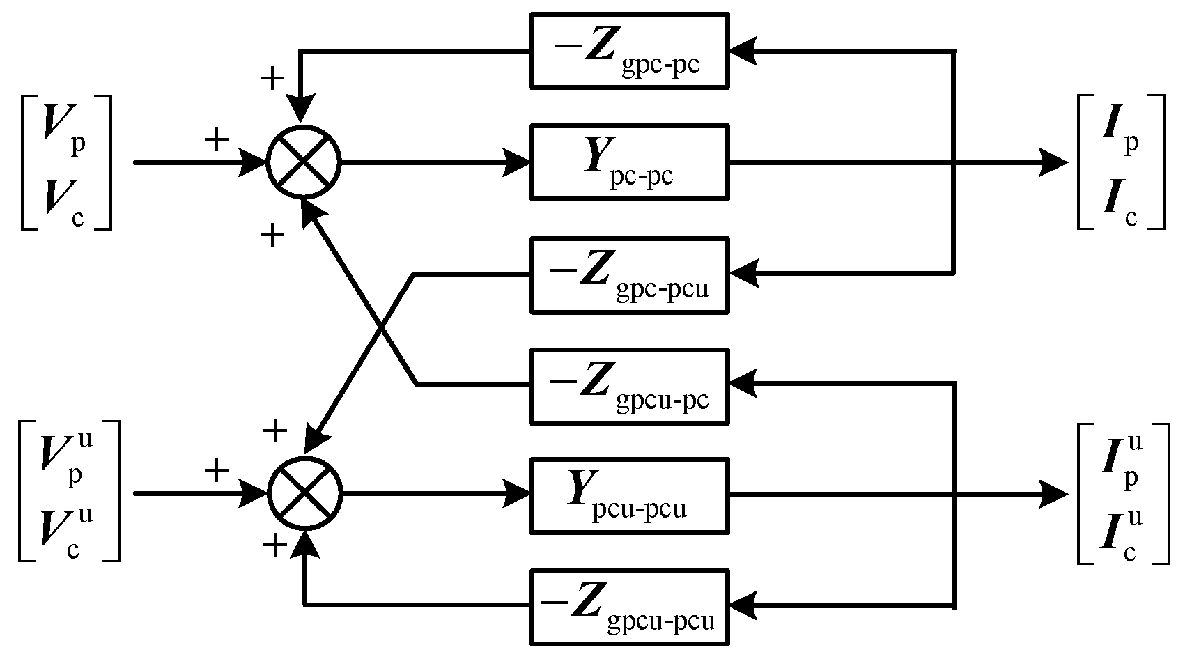
2.3. Impedance Modeling under the Three-Phase Unbalanced Condition

When the grid impedance is unbalanced, the frequency coupling caused by asymmetric dq-axis control and the sequence coupling caused by three-phase unbalance will coexist. Specifically, when the perturbation at a certain frequency is applied to the inverter, due to the frequency-coupling effect, two responses whose frequencies are complementary to twice the fundamental frequency will present. Due to the unbalanced grid impedance, these two responses will also induce corresponding positive or negative sequence responses. However, these responses caused by the unbalanced grid impedance are already very small, so the secondary frequency coupling effect can be ignored [35]. Considering this, the fourth-order impedance matrix is sufficiently accurate to describe the impedance characteristic of the inverter under the unbalanced grid condition.

In the previous section, the impedance model of the inverter under the balanced grid condition was derived. Then, this impedance model can be extended to the unbalanced grid condition by adding extra harmonic components caused by the unbalanced grid impedance, so the four-order impedance matrix of the DSOGI-PLL-based inverter is

$$\left[\begin{array}{c}{\mathit{V}}_{\mathrm{p}}\\ {\mathit{V}}_{\mathrm{c}}^{*}\\ {\mathit{V}}_{\mathrm{pu}}\\ {\mathit{V}}_{\mathrm{cu}}^{*}\end{array}\right]=\left[\begin{array}{cccc}{Z}_{11}& Z_{12}& 0& 0\\ Z_{21}& Z_{22}& 0& 0\\ 0& 0& Z_{33}& 0\\ 0& 0& 0& Z_{44}\end{array}\right]\left[\begin{array}{c}{\mathit{V}}_{\mathrm{p}}\\ {\mathit{V}}_{\mathrm{c}}^{*}\\ {\mathit{V}}_{\mathrm{pu}}\\ {\mathit{V}}_{\mathrm{cu}}^{*}\end{array}\right]$$

(16)

where $Z_{33}=E_1/F_1$, $Z_{44}=E_2/F_2$, $E_1=K_{\mathrm{m}}{V}_{\mathrm{dc}}{G}_{\mathrm{ma}-\mathrm{Vpu}}-1$, $F_1=K_{\mathrm{m}}{V}_{\mathrm{dc}}{G}_{\mathrm{ma}-\mathrm{Ipu}}-Z_{\mathrm{pu}}$, $E_2=K_{\mathrm{m}}{V}_{\mathrm{dc}}{G}_{\mathrm{ma}-\mathrm{Vcu}}-1$, $F_2=K_{\mathrm{m}}{V}_{\mathrm{dc}}{G}_{\mathrm{ma}-\mathrm{Icu}}-Z_{\mathrm{cu}}$, and V_pu and I_pu represent the voltage and current caused by perturbation and the unbalanced grid impedance, respectively. V_cu and I_cu represent the voltage and current caused by the coupled response and the unbalanced grid impedance, respectively. Z_pu and Z_cu represent the unbalanced grid impedance at the perturbation frequency and coupled frequency, respectively.

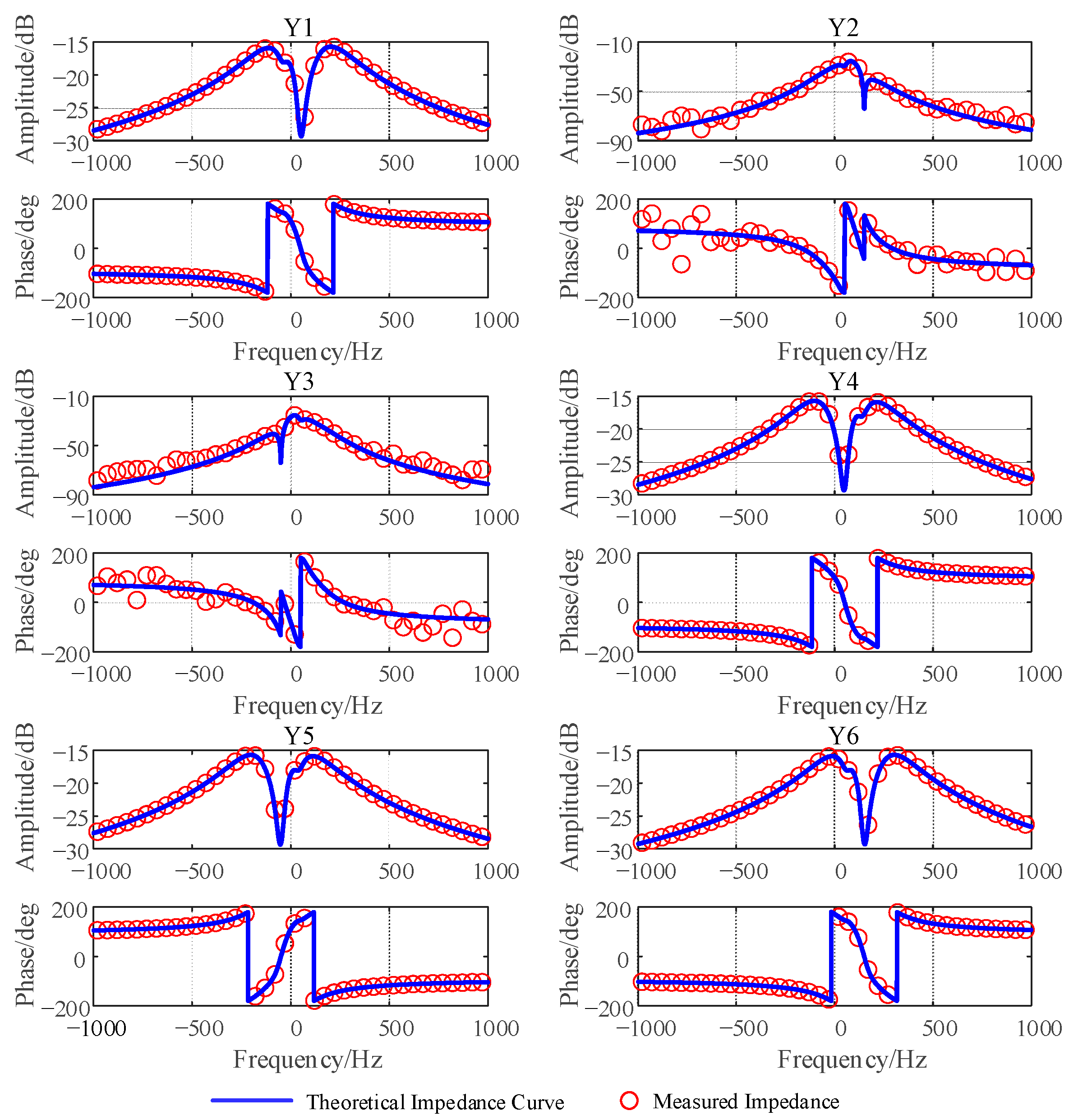
2.4. Simulation Verification of the Impedance Model

To verify the theoretical analysis in Section 2.2 and Section 2.3, based on the control block diagram shown in Figure 2 and Figure 3, a time-domain simulation model was built in MATLAB/Simulink R2023a. The power circuit and control parameters are listed in

Table 1. Parameters and values of the DSOGI-PLL-based inverter system for frequency sweeping.

Parameter	Value	Parameter	Value
Grid voltage	380 V	Grid frequency	50 Hz
DC-link voltage	800 V	Switching frequency	10 kHz
Filter inductance	4 mH	Filter resistance	0.05 Ω
Damping coefficient	1.414	Grid inductance	5 mH
Proportional gain of PLL controller	0.7376	Integral gain of PLL controller	84.352
Proportional gain of current controller	6.47	Integral gain of current controller	4194
d-axis current reference	21.5 A	q-axis current reference	0 A

.

To verify the accuracy of the theoretical frequency-coupled impedance model derived in this section, a series of simulations based on the frequency sweeping method [37] were carried out in MATLAB/Simulink R2023a to obtain the measured impedance of the DSOGI-PLL-based inverter, which is drawn in Figure 4.

Figure 4 indicates that the derived theoretical impedance model is consistent with the frequency sweeping results. Thus, the accuracy of the derived frequency-coupled impedance model is well verified.

3. The Simplified Stability Analysis Method Based on the GNC and Verification

According to the established impedance models of the inverter under the balanced and unbalanced grid conditions, the grid-connected inverter systems are MIMO high-order systems. Therefore, the GNC needs to be adopted for the stability analysis.

3.1. Stability Analysis Method of Inverters under the Balanced Grid Condition

First, the stability analysis of the inverter under the balanced condition is carried out. The block diagram of the DSOGI-PLL-based grid-connected inverter under the balanced grid condition is drawn as shown in Figure 5.

For the stability analysis, we should obtain the transfer functions of the forward path and feedback path. From Figure 5, the transfer function of the forward path is the admittance model of the inverter under the balanced condition, which can be expressed by the inverse matrix of impedance matrix in Equation (15) as

$${\mathit{Q}}_{\mathrm{b}}=\left[\begin{array}{cc}{Y}_{11}& Y_{12}\\ Y_{21}& Y_{22}\end{array}\right]$$

(17)

where Q_b is the admittance matrix.

From Figure 5, the transfer function of the feedback path is the grid impedance model. According to the frequency relationship of perturbation and coupled voltage, we can obtain the transfer function of the feedback path as

$${\mathit{F}}_{\mathrm{b}}=\left[\begin{array}{cc}{Z}_{\mathrm{gp}}& 0\\ 0& Z_{\mathrm{gc}}\end{array}\right]$$

(18)

where Z_gp and Z_gc represent the grid impedance at the perturbation frequency and coupled frequency, respectively.

For such a MIMO system, the closed-loop stability of the grid-connected inverter system can be carried out by analyzing eigenvalues of the return-ratio matrix. Based on the derived transfer functions, the return-ratio matrix can be expressed as

$${\mathit{M}}_{\mathrm{r}}={\mathit{Q}}_{\mathrm{b}}{\mathit{F}}_{\mathrm{b}}=\left[\begin{array}{cc}{Y}_{11}{Z}_{\mathrm{gp}}& Y_{12}{Z}_{\mathrm{gc}}\\ Y_{21}{Z}_{\mathrm{gp}}& Y_{22}{Z}_{\mathrm{gc}}\end{array}\right]$$

(19)

where M_r represents the return-ratio matrix.

Therefore, for inverters under the balanced grid condition, the stability analysis can be carried out by analyzing the eigenvalues of this second-order matrix M_r.

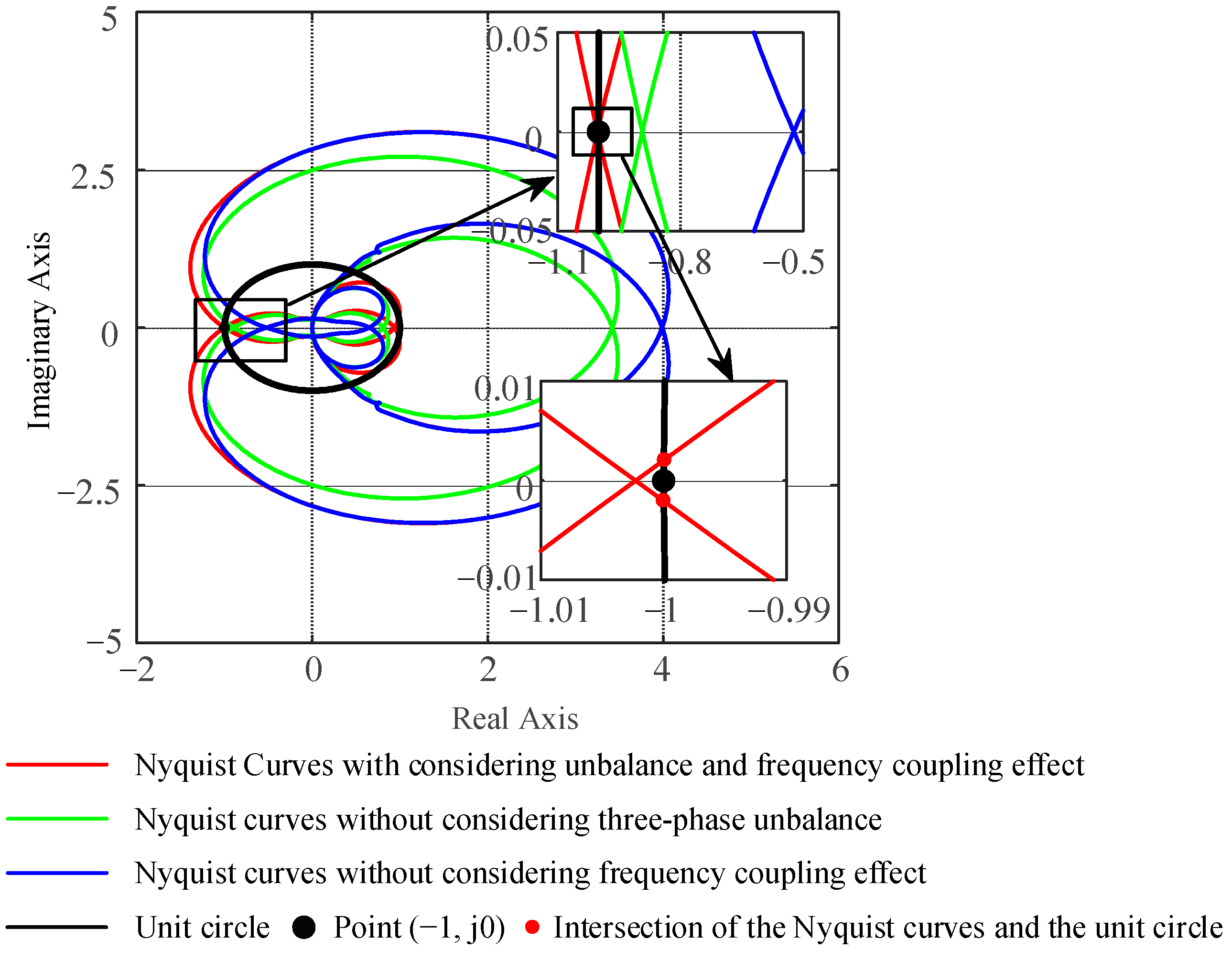
3.2. Stability Analysis Method of Inverters under the Unbalanced Grid Condition

The block diagram of the DSOGI-PLL-based inverter under the unbalanced grid condition is plotted in Figure 6. From Figure 6, the transfer function of the forward path is the frequency-coupled admittance model of the inverter under the unbalanced grid condition, and the feedback path is the unbalanced grid impedance model.

The frequency-coupled impedance model under the unbalanced grid condition has been derived in the previous section. The transfer function of the forward path is the inverse matrix of the impedance matrix in Equation (16):

$${\mathit{Q}}_{\mathrm{u}}=\left[\begin{array}{cccc}{Y}_{11}& Y_{12}& 0& 0\\ Y_{21}& Y_{22}& 0& 0\\ 0& 0& Y_{33}& 0\\ 0& 0& 0& Y_{44}\end{array}\right]$$

(20)

where Q_u is the admittance matrix.

According to the frequency relationship and the symmetric component method, the unbalanced grid impedance model can be derived. Therefore, the transfer function matrix of the feedback path is as follows:

$${\mathit{F}}_{\mathrm{u}}=\left[\begin{array}{cccc}{Z}_{\mathrm{g}11}& 0& Z_{\mathrm{g}13}& 0\\ 0& Z_{\mathrm{g}22}& 0& Z_{\mathrm{g}24}\\ Z_{\mathrm{g}31}& 0& Z_{\mathrm{g}33}& 0\\ 0& Z_{\mathrm{g}42}& 0& Z_{\mathrm{g}44}\end{array}\right]$$

(21)

where Z_g11–Z_g44 represent grid impedance, respectively.

After we obtain the transfer functions of the forward and feedback paths, the analysis of the system stability can be carried out according to the GNC. However, for a four-input four-output high-order system, the GNC is too complicated. In the Nyquist diagram, it is complex and not intuitive to analyze the trajectories of all eigenvalues and whether they encircle the origin. Therefore, we can perform some pre-processing on this fourth-order matrix to simplify the analysis process.

Based on the Schur Complement, the determinant of a high-order matrix can be transformed into the product of determinants of two low-order matrices. Then, according to matrix theory, the determinant problem can be considered as the eigenvalue problem after some processing. Therefore, an eigenvalue problem of a high-order matrix can be transformed into an eigenvalue problem of two low-order matrices. Finally, the stability analysis of this high-order system can be carried out by analyzing the eigenvalues of two low-order matrices.

First, the characteristic matrix Y is written in the form of a block matrix as

$$\mathit{Y}=\mathit{I}+{\mathit{Q}}_{\mathrm{u}}{\mathit{F}}_{\mathrm{u}}=\left[\begin{array}{cc}\mathit{A}& \mathit{B}\\ \mathit{C}& \mathit{D}\end{array}\right]$$

(22)

where $\mathit{A}=\left[\begin{array}{cc}1+Y_{11}{Z}_{\mathrm{g}11}& Y_{12}{Z}_{\mathrm{g}22}\\ Y_{21}{Z}_{\mathrm{g}11}& 1+Y_{22}{Z}_{\mathrm{g}22}\end{array}\right]$, $\mathit{B}=\left[\begin{array}{cc}{Y}_{11}{Z}_{\mathrm{g}13}& Y_{12}{Z}_{g24}\\ Y_{21}{Z}_{g13}& Y_{22}{Z}_{\mathrm{g}24}\end{array}\right]$, $\mathit{C}=\left[\begin{array}{cc}{Y}_{33}{Z}_{\mathrm{g}31}& 0\\ 0& Y_{42}{Z}_{\mathrm{g}42}\end{array}\right]$, and $\mathit{D}=\left[\begin{array}{cc}1+Y_{33}{Z}_{\mathrm{g}33}& 0\\ 0& 1+Y_{44}{Z}_{\mathrm{g}44}\end{array}\right]$.

Therefore, the determinant of matrix Y is equal to the product of the determinant of matrix D and A − BD⁻¹C:

$$\det \left(\mathit{Y}\right)=\det \left(\mathit{D}\right)\det \left(\mathit{A}-\mathit{B}{\mathit{D}}^{-1}\mathit{C}\right)$$

(23)

According to matrix theory, when the determinant of matrix Y is equal to the product of the determinants of matrices D and A − BD⁻¹C, the number of the eigenvalues of matrix Y encircling the origin anticlockwise is equal to the sum of the number of the eigenvalues of matrices D and A − BD⁻¹C encircling the origin anticlockwise. Therefore, the relationship between matrices is

$$\mathrm{enc}\left(\mathit{Y}\right)=\mathrm{enc}\left(\mathit{D}\right)+\mathrm{enc}\left(\mathit{A}-\mathit{B}{\mathit{D}}^{-1}\mathit{C}\right)$$

(24)

where enc(Matrix) represents the number of eigenvalues of the matrix encircling the origin clockwise. The number of eigenvalues of the matrix encircling the origin anticlockwise takes a negative value [38].

Based on matrix theory, matrix D can be expressed as the sum of a unit matrix and matrix D_sub as

$$\mathit{D}=\mathit{I}+{\mathit{D}}_{\mathrm{sub}}=\mathit{I}+\left[\begin{array}{cc}{Y}_{33}{Z}_{\mathrm{g}33}& 0\\ 0& Y_{44}{Z}_{\mathrm{g}44}\end{array}\right]$$

(25)

Then, the number of eigenvalues of the matrix D encircling the origin anticlockwise is equal to the number of eigenvalues of the matrix D_sub encircling the (−1, j0) point anticlockwise. Similarly, another submatrix A − BD⁻¹C can be expressed as

$$\mathit{A}-\mathit{B}{\mathit{D}}^{-1}\mathit{C}=\mathit{I} + {\mathit{A}}_{\mathrm{sub}}$$

(26)

where A_sub represents the equivalent partial matrix.

In summary, based on the Schur Complement and matrix theory, the process of analyzing the stability of higher-order systems is simplified. The stability analysis of the DSOGI-PLL-based inverter under the unbalanced grid condition is transformed into the analysis of two second-order matrix eigenvalues. If the eigenvalues of matrix D_sub and matrix A_sub neither pass through nor encircle anticlockwise the (−1, j0) point, the grid-connected inverter system is stable. And matrix D_sub is equivalent to the traditional model that does not consider the three-phase unbalance and the frequency-coupling effect. This paper aims to investigate the inverter instability phenomenon that cannot be predicted based on the analysis of the traditional model. Therefore, the Nyquist curves based on matrix D_sub will not be shown below to save space. The simplified stability analysis method provided in this section can be applied to similar MIMO systems while ensuring the accuracy of the analysis.

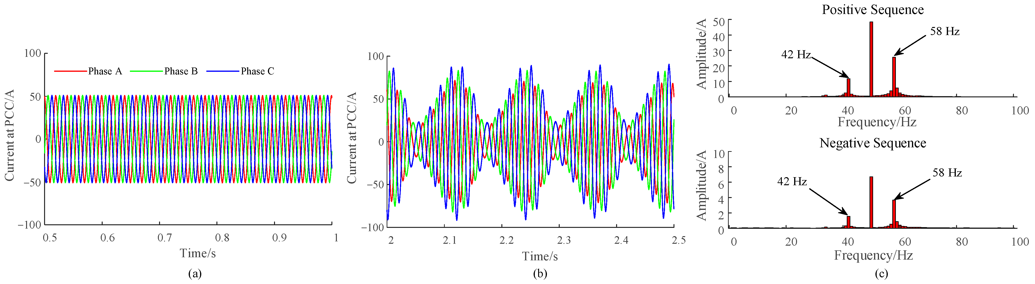
3.3. Simulation Verification of the Stability Analysis Results

To illustrate the importance of considering three-phase unbalance and the frequency-coupling effect for stability analysis of the grid-connected inverter system, the Nyquist curves of the grid-connected inverter system with and without consideration of three-phase unbalance and the frequency-coupling effect are drawn in Figure 7. The main system parameters are listed in

Table 2. Parameters and values of the DSOGI-PLL-based grid-connected inverter system for stability analysis.

Parameter	Value	Parameter	Value
Grid voltage	380 V	Grid frequency	50 Hz
DC-link voltage	800 V	Switching frequency	10 kHz
Filter inductance	1.5 mH	Filter resistance	0.05 Ω
Damping coefficient	1.414	Grid inductance	5 mH
Proportional gain of PLL controller	0.278	Integral gain of PLL controller	11.99
Proportional gain of current controller	1.2	Integral gain of current controller	72.5
d-axis current reference	50 A	q-axis current reference	0 A

. To simulate the three-phase unbalanced grid condition, 2.13 mH extra inductance is added to the a-phase grid impedance, which makes the a-phase grid inductance 7.13 mH.

It can be concluded that with the parameters in Table 2, the Nyquist curves without considering the three-phase unbalance or frequency-coupling effect do not encircle the (−1, j0) point. This indicates that the perturbation cannot trigger any oscillations, and the grid-connected inverter system is stable. But the Nyquist curves considering negative sequence impedance and the frequency-coupling effect encircle the (−1, j0) point. This means that the perturbation will trigger system oscillations. Furthermore, the predicted oscillation frequencies should be 42 Hz and 58 Hz, which correspond to the intersection frequencies of the Nyquist curves and the unit circle, respectively.

Different stability analysis results are given by the Nyquist curves with and without considering the three-phase unbalance and frequency-coupling effect. To verify the above stability analysis results, the time-domain simulation results are shown in Figure 8. At 1.0 s, the a-phase grid inductance is changed from 5 mH to 7.13 mH to simulate the perturbation and unbalanced grid impedance. Figure 8a shows that the inverter can work stably before 1.0 s. Figure 8b illustrates the current waveforms from 2.0 s to 2.5 s, which show when the grid inductance changes suddenly and, with the parameters listed in Table 2, the current starts to oscillate. According to the FFT analysis results of the oscillated current at the PCC shown in Figure 8c, there are several components at different frequencies, with positive sequence components at 42 Hz and 58 Hz and negative sequence components at 42 Hz and 58 Hz.

The time-domain simulation results are consistent with the stability analysis results predicted by the Nyquist curves based on the impedance model considering the three-phase unbalance and frequency-coupling effect. Hence, it can be concluded that the Nyquist curves based on the derived frequency-coupled impedance model in this paper can not only accurately predict the system instability but also the system oscillation frequency. However, the stability analysis given by the Nyquist curves based on the impedance model without considering the three-phase unbalance or frequency-coupling effect cannot predict the instability or oscillation frequency of the system.

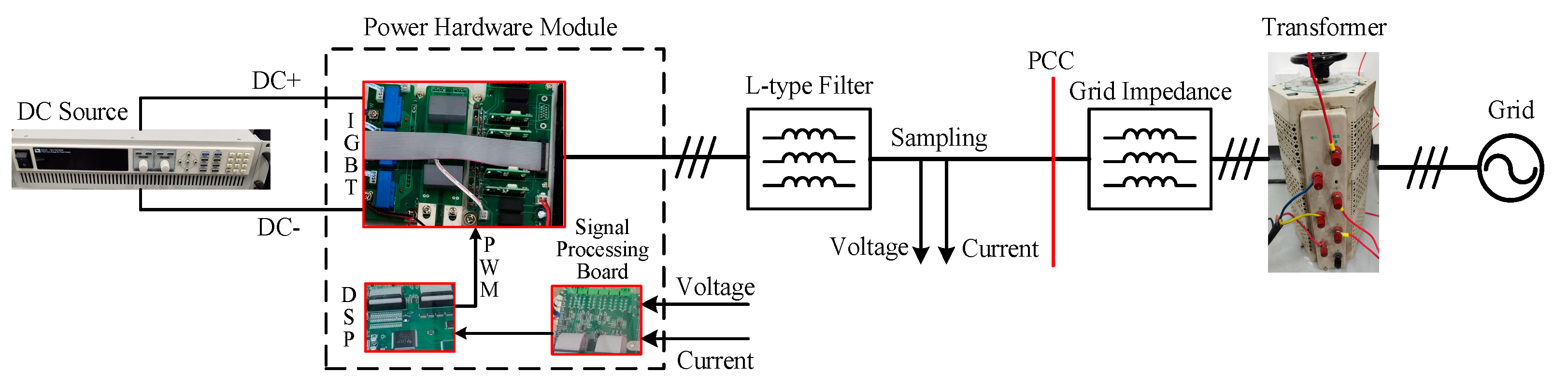
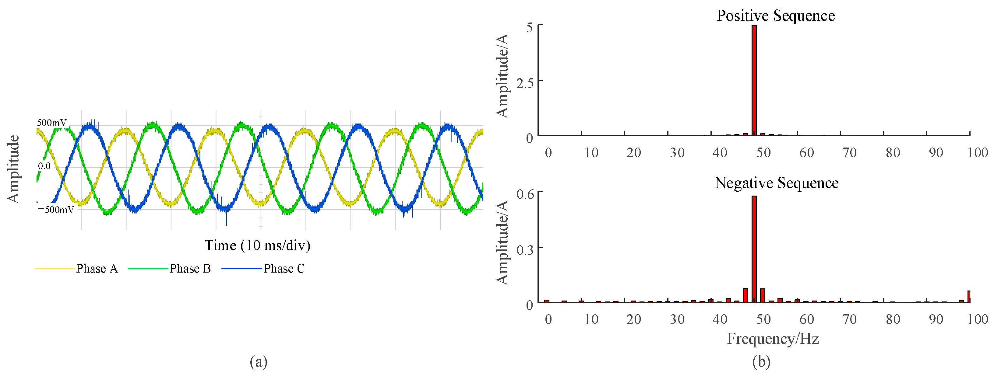
3.4. Experimental Verification of the Stability Analysis Results

In this section, the hardware experimental setup of the grid-connected inverter system is built to further verify the theoretical stability analysis results based on the proposed frequency-coupled impedance model. The AC side is directly connected to the grid through a transformer, and the DC source IT6516C is used to maintain the DC-side voltage. The power hardware module is YXPHM-TP210b-I, which contains the digital signal processor (DSP), IGBTs, and the signal processing board. The digital signal processor chip TMS320F28335 is adopted to control the whole grid-connected system. The experimental setup is illustrated in Figure 9, and the parameters of the experimental setup are listed in

Table 3. Parameters and values of the DSOGI-PLL-based grid-connected inverter system for experimental verification.

Parameter	Value	Parameter	Value
Grid voltage	108 V	Grid frequency	50 Hz
DC-link voltage	300 V	Switching frequency	10 kHz
Filter inductance	2 mH	Filter resistance	0.035 Ω
Damping coefficient	1.414	Grid inductance	6 mH
Proportional gain of PLL controller	1.1246	Integral gain of PLL controller	112.58
Proportional gain of current controller	4.317	Integral gain of current controller	4660
d-axis current reference	5 A	q-axis current reference	0 A

. And to simulate the unbalanced grid condition, an extra 3.0 mH inductance is added to the a-phase grid impedance. Therefore, the grid impedance is unbalanced throughout the hardware experiment.

Based on the proposed stability analysis method in Section 3, we can draw the Nyquist diagram of the grid-connected inverter system with the experimental parameters as shown in Figure 10. In Figure 10, the Nyquist curves of the inverter system with different current loop bandwidths (100 Hz and 500 Hz) are illustrated. When the current loop bandwidth is reduced from 500 Hz to 100 Hz, the grid-connected inverter system becomes unstable. According to the intersection of the Nyquist curves and the unit circle, the predicted oscillation frequencies are 63.5 Hz and 36.5 Hz.

Based on the hardware experimental setup shown in Figure 9 and the experiment parameters listed in Table 3, the hardware experiments of the grid-connected inverter system are carried out to verify the instability phenomenon as the reduction in the current loop bandwidth as well as the corresponding theoretical analysis results. Figure 11 and Figure 12 show the three-phase waveforms and FFT analysis results of the grid-connected current waveforms at the PCC with current loop bandwidths of 500 Hz and 100 Hz, respectively. The conversion ratio of the current probe to measure the grid-connected current is 1 V/10 A.

It can be observed from Figure 11 that the grid-connected inverter system can operate stably when the current loop bandwidth is 500 Hz. Due to the unbalanced grid impedance, an obvious negative sequence harmonic component at 50 Hz exists.

It is obvious from Figure 12 that the current waveforms begin to oscillate when the current loop bandwidth is reduced to 100 Hz. It can be seen from the FFT analysis results that, in addition to the fundamental frequency component, positive sequence components at 34 Hz and 66 Hz and negative sequence components at 34 Hz, 50 Hz, and 66 Hz exist. The main oscillation frequencies of 34 Hz and 66 Hz are very close to the predicted oscillation frequencies of 36.5 Hz and 63.5 Hz. Hence, the experimental results are consistent with the theoretical stability analysis results, which further proves the accuracy of the proposed impedance model and stability analysis method for the inverter under the three-phase unbalanced condition.

4. Analysis of the Influence of Vital System Parameters on System Stability

Based on the frequency-coupled impedance model derived in Section 2 and the simplified stability analysis method proposed in Section 3, the stability of the grid-connected inverter system under the unbalanced condition is analyzed in this section. The influences of the power circuit and control parameters on the system stability are investigated. In this section, the main parameters are listed in Table 1.

4.1. Influence of the Asymmetric Grid Impedance on the System Stability

It is indispensable to analyze the influence of unbalanced grid impedance on system stability. The extra inductances of 0 mH, 1.5 mH, and 3 mH are added to the a-phase grid impedance, respectively, to simulate the unbalanced grid condition. The corresponding Nyquist curves of the inverter system with different extra a-phase grid impedances are plotted in Figure 13. It can be seen that as the a-phase grid impedance increases, the Nyquist curve begins to encircle the point (−1, j0), which indicates that the greater the extent of the grid inductance asymmetry, the higher the risk of system instability.

4.2. Influence of the Control Parameter on System Stability

In this subsection, the influences of the current loop bandwidth and the DSOGI-PLL parameters on the system stability are investigated. Similar to Section 4.1, the extra inductance of 1.5 mH is added to the a-phase grid impedance to simulate the unbalanced grid condition, and the other parameters are listed in Table 1.

The Nyquist curves of the inverter with different current loop bandwidths are shown in Figure 14. As the bandwidth of the current loop increases, the Nyquist curves no longer encircle the point (−1, j0), which means that as the bandwidth of the current loop increases, the grid-connected system’s stability is continuously strengthened. Therefore, when designing parameters of the current loop, the current loop bandwidth can be appropriately designed to be relatively larger within design principles.

For the SRF-PLL, the only factor that affects its characteristics is the PI controller parameter. However, the DSOGI-PLL is composed of two SOGIs and the subsequent PLL, so the parameters that affect its characteristics include the damping coefficient in SOGI and the control bandwidth of the PLL. Therefore, the influences of the damping coefficient and control bandwidth of the PLL (B_PLL) on system stability should be analyzed separately.

The Nyquist curves for different damping coefficients are shown in Figure 15a. It can be seen that as the damping coefficient increases, the Nyquist curves are closer to the point (−1, j0), which means that the larger the damping coefficient, the higher the risk of system instability. The Nyquist curves for different B_PLLs are shown in Figure 15b. It can be observed that as the B_PLL increases, the Nyquist curves move closer to the point (−1, j0), which means that as the B_PLL increases, the stability margin of the system reduces.

4.3. Recommendations for Parameter Design

Based on the analysis results in Section 4.1 and Section 4.2, some recommendations for the parameter design for the inverter under the unbalanced grid condition are given as follows.

(1)

As analyzed in Section 4.1, the stability margin of the inverter is smaller under greater grid impedance unbalance. Therefore, for a inverter that may work under the unbalanced grid condition, the parameter design should be more conservative.

(2)

For a inverter under the unbalanced grid condition, the current loop bandwidth should be larger than that under the balanced grid condition. However, a larger current bandwidth may introduce oscillation problems at medium and high frequencies. Therefore, the setting of the current loop bandwidth should be considered to satisfy the stability margin requirement within a wide frequency band.

(3)

According to the analysis results in Section 4.2, it can be concluded that dynamic performance cannot only be pursued when designing the DSOGI-PLL of the grid-connected inverter system. It is necessary to appropriately reduce the damping coefficient and control bandwidth of the PLL to improve the stability of the whole grid-connected system.

5. Conclusions

In this paper, the stability of the DSOGI-PLL-based grid-connected inverter under the unbalanced grid condition is investigated. Considering the frequency-coupling effect, frequency-coupled impedance models of the DSOGI-PLL-based grid-connected inverter under balanced and unbalanced grid conditions are derived. To analyze the stability under the unbalanced condition, a simplified stability analysis method for the MIMO system is proposed and the stability analysis is carried out based on this method. Based on the proposed impedance model and analysis method, the influences of system parameters on the system stability are investigated. According to the analysis results, parameter design recommendations are summarized to provide guidance for practical engineering and other researchers. Finally, the accuracy of the proposed frequency-coupled impedance model and the effectiveness of the simplified stability analysis method have been well validated. The system’s critical instability points and oscillation frequencies can be accurately predicted. The proposed impedance modeling method and stability analysis method have broad application prospects for modeling and analyzing other power electronic devices. The research in this paper can provide a general theoretical basis for the stability analysis of inverters under balanced and unbalanced grid conditions.

References

1. Kojima, H.; Nagasawa, K.; Todoroki, N.; Ito, Y.; Matsui, T.; Nakajima, R. Influence of renewable energy power fluctuations on water electrolysis for green hydrogen production. Int. J. Hydrogen Energy 2023, 12, 4572–4593. [Google Scholar] [CrossRef]
2. Ghasemi, M.A.; Zarei, S.F.; Sohrabi, Z.; Blaabjerg, F.; Peyghami, S. An Observer-Based Current Sensor-Less Control Scheme for Grid-Following Converters. Appl. Sci. 2022, 12, 7749. [Google Scholar] [CrossRef]
3. Huang, Y.; Yuan, X.; Hu, J.; Zhou, P.; Wang, D. DC-Bus voltage control stability affected by AC-bus voltage control in VSCs connected to weak AC grids. IEEE J. Emerg. Sel. Top. Power Electron. 2016, 2, 445–458. [Google Scholar] [CrossRef]
4. Saha, S.; Saleem, M.I.; Roy, T.K. Impact of high penetration of renewable energy sources on grid frequency behaviour. Int. J. Electr. Power Energy Syst. 2023, 145, 108701. [Google Scholar] [CrossRef]
5. Meraj, S.T.; Yu, S.S.; Rahman, S.; Hasan, K.; Lipu, M.H.; Trinh, H. Energy management schemes, challenges and impacts of emerging inverter technology for renewable energy integration towards grid decarbonization. J. Clean. Prod. 2023, 405, 137002. [Google Scholar] [CrossRef]
6. Adib, A.; Mirafzal, B.; Wang, X.; Blaabjerg, F. On Stability of Voltage Source Inverters in Weak Grids. IEEE Access 2018, 6, 4427–4439. [Google Scholar] [CrossRef]
7. Rolán, A.; Bogarra, S.; Bakkar, M. Integration of Distributed Energy Resources to Unbalanced Grids Under Voltage Sags with Grid Code Compliance. IEEE Trans. Smart Grid 2022, 1, 355–366. [Google Scholar] [CrossRef]
8. Nian, H.; Yang, H. Impedance modeling and stability analysis of grid-connected inverters under unbalanced operation conditions. Autom. Control. Electr. Power Syst. 2016, 10, 76–83. [Google Scholar]
9. Yoon, S.-J.; Tran, T.V.; Kim, K.-H. Stability Assessment of Current Controller with Harmonic Compensator for LCL-Filtered Grid-Connected Inverter under Distorted Weak Grid. Appl. Sci. 2021, 11, 212. [Google Scholar] [CrossRef]
10. Harnefors, L.; Wang, X.; Yepes, A.G.; Blaabjerg, F. Passivity-based stability assessment of grid-connected VSCs—An overview. IEEE J. Emerg. Sel. Top. Power Electron. 2016, 1, 116–125. [Google Scholar] [CrossRef]
11. Alenius, H.; Roinila, T.; Luhtala, R.; Messo, T.; Burstein, A.; de Jong, E.; Fabian, A. Hardware-in-the-Loop Methods for Stability Analysis of Multiple Parallel Inverters in Three-Phase AC Systems. IEEE J. Emerg. Sel. Top. Power Electron. 2021, 6, 7149–7158. [Google Scholar] [CrossRef]
12. Sajadi, A.; Rañola, J.A.; Kenyon, R.W.; Hodge, B.-M.; Mather, B. Dynamics and Stability of Power Systems with High Shares of Grid-Following Inverter-Based Resources: A Tutorial. IEEE Access 2023, 11, 29591–29613. [Google Scholar] [CrossRef]
13. Mohammadi, F.D.; Vanashi, H.K.; Feliachi, A. State-Space Modeling, Analysis, and Distributed Secondary Frequency Control of Isolated Microgrids. IEEE Trans. Energy Convers. 2018, 1, 155–165. [Google Scholar] [CrossRef]
14. Zhu, Y.; Gu, Y.; Li, Y.; Green, T.C. Participation Analysis in Impedance Models: The Grey-Box Approach for Power System Stability. IEEE Trans. Power Syst. 2022, 1, 343–353. [Google Scholar] [CrossRef]
15. Sun, J. Impedance-Based Stability Criterion for Grid-Connected Inverters. IEEE Trans. Power Electron. 2011, 11, 3075–3078. [Google Scholar] [CrossRef]
16. Shah, S.; Koralewicz, P.; Gevorgian, V.; Wallen, R. Sequence Impedance Measurement of Utility-Scale Wind Turbines and Inverters—Reference Frame, Frequency Coupling, and MIMO/SISO Forms. IEEE Trans. Energy Convers. 2022, 1, 75–86. [Google Scholar] [CrossRef]
17. Babu, Y.N.; Padhy, N.P. Investigation of Damping Effect of PLL on Low-Frequency Harmonic Stability of Grid-Tied Inverter With αβ and dq Current Control Schemes. IEEE J. Emerg. Sel. Top. Power Electron. 2022, 1, 1046–1060. [Google Scholar] [CrossRef]
18. Song, Y.; Wu, S. Research on Low-Frequency Oscillation Damping Control of Wind Storage System Based on Pareto and Improved Particle Swarm Algorithm. Appl. Sci. 2023, 13, 10054. [Google Scholar] [CrossRef]
19. Mohammed, N.; Zhou, W.; Bahrani, B. Double-Synchronous-Reference-Frame-Based Power-Synchronized PLL-Less Grid-Following Inverters for Unbalanced Grid Faults. IEEE Open J. Power Electron. 2023, 4, 474–486. [Google Scholar] [CrossRef]
20. Bakhshizadeh, M.K.; Wang, X.; Blaabjerg, F.; Hjerrild, J.; Kocewiak, Ł.; Bak, C.L.; Hesselbæk, B. Couplings in Phase Domain Impedance Modeling of Grid-Connected Converters. IEEE Trans. Power Electron. 2016, 10, 6792–6796. [Google Scholar]
21. Wang, X.; Blaabjerg, F. Harmonic stability in power electronic-based power systems: Concept, modeling, and analysis. IEEE Trans. Smart Grid 2019, 3, 2858–2870. [Google Scholar] [CrossRef]
22. Cecati, F.; Becker, J.K.M.; Pugliese, S.; Zuo, Y.; Liserre, M.; Paolone, M. LTP Modeling and Analysis of Frequency Coupling in PLL-Synchronized Converters for Harmonic Power Flow Studies. IEEE Trans. Smart Grid 2023, 4, 2890–2902. [Google Scholar] [CrossRef]
23. Nian, H.; Xu, Y.; Chen, L.; Li, G. Frequency coupling characteristic modeling of grid-connected inverter and system stability analysis. Proc. CSEE 2019, 5, 1421–1431. [Google Scholar]
24. Huang, L.; Wu, C.; Zhou, D.; Blaabjerg, F. A Double-PLLs-Based Impedance Reshaping Method for Extending Stability Range of Grid-Following Inverter Under Weak Grid. IEEE Trans. Power Electron. 2022, 4, 4091–4104. [Google Scholar] [CrossRef]
25. Guo, X.; Zhang, S.; Yan, Z.; Wei, Y.; Hu, X. A Novel Phase-Locked Loop Structure to Enhance Converter Stability in Weak Grids. IEEE Trans. Power Electron. 2023, 11, 13855–13865. [Google Scholar] [CrossRef]
26. Nian, H.; Hu, B.; Xu, Y.; Wu, C.; Chen, L.; Blaabjerg, F. Analysis and Reshaping on Impedance Characteristic of DFIG System Based on Symmetrical PLL. IEEE Trans. Power Electron. 2020, 11, 11720–11730. [Google Scholar] [CrossRef]
27. Arya, S.R.; Patel, M.M.; Alam, S.J.; Srikakolapu, J.; Giri, A.K. Phase lock loop–based algorithms for DSTATCOM to mitigate load created power quality problems. Int. Trans. Electr. Energ. Syst. 2020, 30, e12161. [Google Scholar] [CrossRef]
28. Yang, H.; Eggers, M.; Teske, P.; Dieckerhoff, S. Comparative Stability Analysis and Improvement of Grid-Following Converters Using Novel Interpretation of Linear Time-Periodic Theory. IEEE J. Emerg. Sel. Top. Power Electron. 2022, 6, 7049–7061. [Google Scholar] [CrossRef]
29. Céspedes, M.; Sun, J. Methods for stability analysis of unbalanced three-phase systems. In Proceedings of the 2012 IEEE Energy Conversion Congress and Exposition (ECCE), Raleigh, NC, USA, 15–20 September 2012; pp. 3090–3097. [Google Scholar]
30. Liu, W.; Wang, X.; Blaabjerg, F. Modeling of unbalanced three-phase grid-connected converters with decoupled transfer functions. In Proceedings of the 2018 International Power Electronics Conference (IPEC-Niigata 2018-ECCE Asia), Niigata, Japan, 20–24 May 2018; pp. 3164–3169. [Google Scholar]
31. Ugalde-Loo, C.E.; Acha, E.; Licéaga-Castro, E. Analysis of the damping characteristics of two power electronics-based devices using ‘individual channel analysis and design. Appl. Math. Model. 2018, 59, 527–545. [Google Scholar] [CrossRef]
32. Wu, W.; Liu, J.; Li, Y.; Blaabjerg, F. Individual channel design-based precise analysis and design for three-phase grid-tied inverter with LCL filter under unbalanced grid impedance. IEEE Trans. Power Electron. 2020, 5, 5381–5396. [Google Scholar] [CrossRef]
33. Jin, W.; Li, Y.; Sun, G.; Chen, X.; Gao, Y. Stability analysis method for three-phase multi-functional grid-connected inverters with unbalanced local loads considering the active imbalance compensation. IEEE Access 2018, 6, 54865–54875. [Google Scholar] [CrossRef]
34. Zhang, H.; Harnefors, L.; Wang, X.; Gong, H.; Hasler, J. Stability analysis of grid-connected voltage-source converters using SISO modeling. IEEE Trans. Power Electron. 2019, 8, 8104–8117. [Google Scholar] [CrossRef]
35. Zhang, C.; Molinas, M.; Rygg, A.; Lyu, J.; Cai, X. Harmonic transfer function-based impedance modeling of a three-phase VSC for asymmetric ac grid stability analysis. IEEE Trans. Power Electron. 2019, 12, 12552–12566. [Google Scholar] [CrossRef]
36. Yang, C.; Xin, H.; Gong, Z.; Dong, W.; Jyu, P.; Xu, L. Complex circuit analysis and investigation on applicability of generalized-impedance-based stability criterion for grid-connected converter. Proc. CSEE 2020, 15, 4744–4757. [Google Scholar]
37. Liu, W.; Lu, Z.; Wang, X.; Xie, X. Frequency-coupled admittance modelling of grid-connected voltage source converters for the stability evaluation of subsynchronous interaction. IET Renew. Power Gener. 2018, 2, 285–295. [Google Scholar] [CrossRef]
38. Jiang, C.; Shi, P.; Huang, W.; Zhou, J.; Gan, D. Parameter setting method for 26multi-band power system stabilizer considering multiple oscillation modes. Autom. Electr. Power Syst. 2020, 4, 142–149. [Google Scholar]
Figure 1. The flowchart of the analysis steps in this paper.
Applsci 13 12441 g001
Figure 2. The basic structure of the DSOGI-PLL-based inverter.
Applsci 13 12441 g002
Figure 3. The structure of the SOGI and DSOGI-PLL.
Applsci 13 12441 g003
Figure 4. Comparison of theoretical and measured impedance of the DSOGI-PLL-based inverter.
Applsci 13 12441 g004
Figure 5. The block diagram of the DSOGI-PLL-based inverter under the balanced grid condition.
Applsci 13 12441 g005
Figure 6. The block diagram of the DSOGI-PLL-based inverter under the unbalanced grid condition.
Applsci 13 12441 g006
Figure 7. Comparison of different Nyquist curves of the DSOGI-PLL-based inverter.
Applsci 13 12441 g007
Figure 8. Current waveform at the PCC with different a-phase grid inductances: (a) Waveform from 0.5 to 1.0 s with 5 mH a-phase grid inductance (b) Waveform from 2.0 to 2.5 s with 7.13 mH a-phase grid inductance. (c) FFT analysis results of the current from 2.0 to 3.0 s.
Applsci 13 12441 g008
Figure 9. The configuration of the experimental setup.
Applsci 13 12441 g009
Figure 10. Nyquist curves of the inverter system with different current loop bandwidths for the experimental parameters.
Applsci 13 12441 g010
Figure 11. Experimental current and FFT analysis results when the current loop bandwidth is 500 Hz: (a) Current waveforms; (b) FFT analysis results for positive and negative sequence.
Applsci 13 12441 g011
Figure 12. Experimental current and FFT analysis results when the current loop bandwidth is 100 Hz (a) Current waveforms (b) FFT analysis results for positive and negative sequences.
Applsci 13 12441 g012
Figure 13. Nyquist curves of the inverter system with different amounts of extra a-phase grid impedance.
Applsci 13 12441 g013
Figure 14. Nyquist curves of the DSOGI-PLL-based inverter with different current loop bandwidths.
Applsci 13 12441 g014
Figure 15. Nyquist curves of the DSOGI-PLL-based inverter with different parameters: (a) The DSOGI-PLL with different damping coefficients. (b) The DSOGI-PLL with different BPLLs.
Applsci 13 12441 g015