Adaptive Clutter Intelligent Suppression Method Based on Deep Reinforcement Learning

Abstract

In the complex clutter background, the clutter center frequency is not fixed, and the spectral width is wide, which leads to the performance degradation of the traditional adaptive clutter suppression method. Therefore, an adaptive clutter intelligent suppression method based on deep reinforcement learning (DRL) is proposed. Each range cell to be detected is regarded as an independent intelligence (agent) in the proposed method. The clutter environment is interactively learned using a deep learning (DL) process, and the filter parameter optimization is positively motivated by the reinforcement learning (RL) process to achieve the best clutter suppression effect. The suppression performance of the proposed method is tested on simulated and real data. The experimental results indicate that the filter notch designed by the proposed method is highly matched with the clutter compared with the existing adaptive clutter suppression methods. While suppressing the clutter, it has a higher amplitude-frequency response to signals at non-clutter frequencies, thus reducing the loss of the target signal and maximizing the output signal-to-clutter and noise rate (SCNR).

1. Introduction

Radar detects targets by transmitting electromagnetic waves. Echo signals contain not only target information but also complex background environmental reflection echoes, which are called clutter and can seriously affect radar target detection performance [1,2,3]. These clutter signals usually have high energy, which can easily mask the target signal, resulting in it being difficult for the radar system to efficiently distinguish the target from the clutter [4,5]. Therefore, clutter suppression technology is indispensable for radar target detection and has always been an important research direction in the radar field [6].

For a long time, many scholars have conducted extensive research on radar clutter suppression methods, mainly focusing on two categories: the subspace decomposition method and the time-domain cancellation method. The subspace decomposition method is based on the difference between clutter and target signal aggregation characteristics in the subspace and achieves clutter suppression by separating the clutter subspace. It can be divided into eigen value decomposition (EVD) [7,8] and singular value decomposition (SVD) [9,10,11,12]. The SVD method performs better than the EVD method in clutter suppression. The SVD suppression method is performed by constructing a Hankel matrix from the time-domain signal of the radar echo, and then an SVD of this matrix is performed. The suppression of the clutter is achieved by setting the first few larger singular values to zero and then reconstructing them. In fact, the target energy is not always smaller than the clutter signal energy, which resulted in a much higher probability of target miscancellation. Article [13] proposed a combination of singular value decomposition and the fractional Fourier transform (FRFT). Through the optimal FRFT transform, the target signal and clutter signal in the echo signal can be separated in the fractional domain, and the SVD is used in the fractional domain to further improve the distinction between the target signal and clutter. However, this method can only be used when the signal-to-clutter ratio (SCR) is high and the Doppler modulation of the target echo signal is approximately linear frequency modulation (LFM). When the SCR is low, it is easy to extract the clutter signal and suppress the target signal. Article [14] proposed a method combining SVD and a projection algorithm, constructing the clutter space of the neighboring cells to be detected. In the projection space, SVD is used on the clutter space to achieve clutter suppression. However, this algorithm requires that the range cells to be detected have a strong correlation with the neighboring cells; otherwise, it is difficult to achieve the desired suppression effect.

Time-domain cancellation methods include cyclic cancellation [15,16], Moving Target Indications (MTI) [17,18], Adaptive Moving Target Indications (AMTI) [19,20], etc. The cyclic cancellation method first estimates the parameters of the clutter signal model, thereby reconstructing the sea clutter in the time domain and subtracting it from the echo signal to achieve clutter suppression. However, it is necessary to establish a model that matches the real clutter characteristics. Due to the fact that the existing clutter models are not universal, the effect of clutter suppression in practical applications is not significant, and the cyclic elimination method faces certain difficulties in practical engineering applications. The traditional MTI method mainly uses two-pulse and three-pulse cancellers to suppress stationary clutter. Its implementation method is to generate a depression at zero frequency to eliminate the stationary clutter with a zero-frequency center. This method is simple to implement, but it is not effective for clutter with a certain Doppler frequency, such as sea clutter and meteorological clutter, which have complex non-stationary, nonlinear, and non-Gaussian “three non” characteristics [21]. The design idea of the AMTI method is to find a set of filter coefficients that can effectively suppress clutter and ensure the target signal passes through without loss. The eigenvector method is the main optimization design method of the MTI filter. It automatically adjusts the filter notch by adaptively estimating the clutter center frequency and spectral width to achieve the suppression of dynamic and static clutter, but the method requires that the clutter data for constructing the covariance matrix satisfy the independent and identically distributed (IID) condition. However, the actual clutter characteristics are complicated and variable by the environmental changes, which do not satisfy the IID conditions, resulting in the limited performance of traditional AMTI clutter suppression methods.

In recent years, with the continuous development and application of deep learning, the application of intelligent methods to the radar field has achieved good application prospects and become a hot spot of current research. Article [22] introduced a deep convolutional neural network (CNN) to classify and identify the clutter amplitude distribution, obtaining sufficient clutter sample data obeying IID and improving the performance of the AMTI clutter suppression method. However, the experiment was only conducted in a specific clutter background situation, and its model generalization ability may be insufficient when facing different sea state and environmental changes. Article [23] utilized a CNN to train sea echo signals, constructed a clutter autocorrelation matrix by estimating parameters related to the sea clutter power spectrum, designed filter weight coefficients that match the clutter, and achieved the suppression of sea clutter. However, the method relies on the dataset and valid labels to train the CNN, and acquiring and labeling the radar echo data is very time-consuming and highly dependent on manual intervention.

Given the limitations of traditional and intelligent clutter suppression methods, including poor adaptability in complex environments, limited generalization capabilities, and a heavy reliance on manual intervention, an adaptive clutter intelligent suppression method based on deep reinforcement learning (DRL) is proposed, which achieved online adaptive filter parameter adjustment of to-be-detected cell in complex environments for the first time. Traditional methods usually rely on fixed rules and a large number of manual interventions, which make it difficult to adapt to changing environments. In contrast, an intelligent environment perception method of deep learning (DL) is introduced in this method, which enables each detected cell (agent) to have the ability to perceive and learn the complex environment online, achieve the feature extraction of environmental observation data, and automatically adjust the filter parameters through reinforcement learning (RL), significantly reducing the manual involvement. Through the innovatively designed reward and punishment mechanism and the introduction of a greedy strategy, agents interact with the environment to learn the optimal filter parameters, achieve effective suppression of clutter, increase the signal-to-clutter and noise rate (SCNR), and enhance target detection performance.

2. Signal Model

Assuming that the radar transmitter transmits an LFM signal, the radar pulse width (PW) is $T_p$, the pulse repetition interval (PRI) is $T_r$, the frequency modulation (FM) bandwidth is $B$, the LFM rate is defined as $\mu =B/T_{\mathrm{p}}$, and the carrier frequency is $f_{\mathrm{c}}$, then the radar transmits the signal in the $n$th transmit cycle as the following Equation (1):

$$S_n(t)=\mathrm{rect}\left[{\displaystyle \frac{t-n{T}_r}{T_p}}\right]\exp \left[\mathrm{j}2\pi (f_{\mathrm{c}}(t-n{T}_r)+{\displaystyle \frac{1}{2}}\mu {(t-n{T}_r)}^2)\right]$$

(1)

where $\mathrm{rect}\left[{\displaystyle \frac{t-n{T}_r}{T_p}}\right]=1,\left|t\right|\le {\displaystyle \frac{T_p}{2}}+n{T}_r$. At the moment $t=0$, the distance of the target relative to the radar is $R_0$, and the speed of uniform motion is $v$. At this time, the echo delay of the target can be expressed as $\begin{array}{c}\tau =2(R_0-v{t}_n)/c\end{array}$, $t_n=n{T}_{\mathrm{r}}$, $c$ is the speed of light, and the echo model of a single target in the $n$th cycle can be obtained as

$$\begin{array}{c}{x}_{nr}(t)=\mathrm{rect}({\displaystyle \frac{t-n{T}_r-\tau }{T_p}})\exp [\mathrm{j}2\pi (f_{\mathrm{c}}(t-n{T}_r-\tau )+{\displaystyle \frac{1}{2}}\mu {(t-n{T}_r-\tau )}^2)]+c(t)+n(t)\end{array}$$

(2)

where $c(t)$ is the clutter, and $n(t)$ is the Gaussian white noise generated by the receiver. Based on Equation (2), the fast- and slow-time-dimensional echo matrix of the echo signal is established. Fast-time-dimensional pulse compression of the matrix can be obtained as

$$X_{\mathrm{c}}=\left[\begin{array}{cccc}{x}_1(1)\exp (\mathrm{j}{f}_d{T}_r)& x_1(2)\exp (\mathrm{j}{f}_d{T}_r)& \cdots & x_1(L)\exp (\mathrm{j}{f}_d{T}_r)\\ x_2(1)\exp (\mathrm{j}2f_d{T}_r)& x_2(2)\exp (\mathrm{j}2f_d{T}_r)& \cdots & x_2(L)\exp (\mathrm{j}2f_d{T}_r)\\ ⋮& ⋮& ⋮& ⋮\\ x_N(1)\exp (\mathrm{j}N{f}_d{T}_r)& x_N(2)\exp (\mathrm{j}N{f}_d{T}_r)& \cdots & x_N(L)\exp (\mathrm{j}N{f}_d{T}_r)\end{array}\right]$$

(3)

where $X_{\mathrm{c}}$ is the echo data matrix of $N\times L$, $N$ is the number of pulse accumulations, $L$ is the number of range cells, $\mathrm{j}$ is the imaginary unit, and $f_{\mathrm{d}}$ is the Doppler frequency of the echo signal.

3. MTI Filter Based on the Eigenvector Method

It is usually assumed that the power spectrum of the clutter obeys a Gaussian distribution, $f_0$ is the spectral center, ${\sigma }_f$ is the spectral width, and its power spectrum is expressed as

$$C(f)={\displaystyle \frac{1}{2\pi {\sigma }_f}}\exp (-{\displaystyle \frac{(f-f_0)}{2{\sigma }_f^2}})$$

(4)

According to Wiener filtering theory, clutter is usually regarded as a smooth random process, and its frequency domain suppression characteristics can be analyzed using the power spectral function. There is a Fourier transform relationship between the power spectral function and the autocorrelation function. Therefore, the clutter autocorrelation function is represented by the following Equation (5):

$$r_c(m,n)={\displaystyle {\int }_{-\infty }^{+\infty }C(f)e^{j2\pi f(t_m-t_n)}}df={\displaystyle {\int }_{-\infty }^{+\infty }\frac{1}{2\pi {\sigma }_f}\exp (-\frac{(f-f_0)}{2{\sigma }_f^2})e^{j2\pi f(t_m-t_n)}}df$$

(5)

from equation ${\displaystyle \frac{1}{2\pi }}{\displaystyle {\int }_{-\infty }^{+\infty }{e}^{-a{x}^2}{e}^{j\xi x}}df={\displaystyle \frac{1}{\sqrt{2a}}}\exp {\displaystyle \frac{{\xi }^2}{4a}}$, we can derive Equation (6) as

$$r_c(m,n)=e^{-2{\pi }^2{\sigma }_f^2{\tau }_{mn}^2}{e}^{j2\pi f_0{\tau }_{mn}}$$

(6)

where ${\tau }_{mn}=t_m-t_n$ is time-dependent.

The power spectral center ${\widehat{f}}_0$ estimated based on FFT selection [24] and the spectral width ${\widehat{\sigma }}_f$ estimated based on integration method [24] are substituted into Equation (6), and the clutter autocorrelation matrix $R_c$ is constructed according to the following Equation (7):

$$R_c=\left[\begin{array}{cccc}{r}_c(0,0)& r_c(0,1)& \cdots & r_c(0,N-1)\\ r_c(1,0)& r_c(1,1)& \cdots & r_c(1,N-1)\\ ⋮& ⋮& \ddots & ⋮\\ r_c(N-1,0)& r_c(N-1,1)& \cdots & r_c(N-1,N-1)\end{array}\right]$$

(7)

from the eigenequation $R_c{w}_n={\lambda }_n{w}_n$, $n=0,1,\cdots ,N$, the eigenvalue decomposition of $R_c$ is calculated to compute the eigenvalues and eigenvectors, where $w_n$ is the eigenvector corresponding to the eigenvalue ${\lambda }_n$. Ranking the eigenvalues ${\lambda }_n$ in ascending order yields ${\lambda }_0\le {\lambda }_1\le \cdots {\lambda }_n$. Article [18] proved that the eigenvector $w_0$, corresponding to the smallest eigenvalue ${\lambda }_0$ obtained by the eigenvalue decomposition of the clutter autocorrelation matrix, is the optimal weight coefficients $W_{opt}=[w_1,w_2,\cdots ,w_m]$ of the filter, and $m$ is the filter orders; using the optimal weight coefficients $W_{opt}$ obtained above to filter the echo data matrix, the output signal is expressed as

$$Y_{ij}=X\cdot W_{opt}^T$$

(8)

In the above Equation (8), $X=[x_{i,j},x_{(i+1),j},\cdots ,x_{(i+m-1),j}]$ represents the echo sequence of successive $m$ pulses from the $i$th pulse to the $i+m-1$ pulse at the $j$th range cell of the echo data matrix; $Y_{ij}$ represents the filtered value of the radar echo data of the $i$th pulse, the $j$th range cell.

According to the above analysis, the performance of the MTI filter based on the eigenvector method in the time domain is the clutter signal multiplied by the optimal weight coefficient $W_{opt}$ to achieve clutter suppression. In the frequency domain, according to the spectrum characteristics of the clutter signal, the filter notch is in the center of the clutter frequency $f_0$, and the notch width is ${\sigma }_f$. The wider the spectral width of the clutter, the wider the width of the filter notch is designed, and the shallower the notch depth will be. The narrower the spectral width of the clutter, the narrower the width of the filter notch, and the deeper the notch depth will be. When the filter notch is consistent with the spectrum width of the clutter, the filtering effect is optimal, and the filter parameters are the optimal parameters for this range cell.

In practical applications, the MTI filter based on the eigenvector method is highly dependent on the a priori knowledge of the clutter information. In order to obtain the best filtering effect, it is necessary to accurately estimate the clutter. Therefore, the accuracy of the clutter estimation is directly related to the performance of the designed filter. However, complex environments may lead to variable clutter characteristics and the clutter characteristics of different range cells may differ significantly, which increases the difficulty of obtaining accurate a priori knowledge, resulting in poor adaptive clutter suppression effect. How to accurately obtain the clutter information to adjust the filter parameters is a key issue in adaptive filter design. Deep reinforcement learning (DRL) provides another new attempt to accurately obtain the sea clutter information and adjust the filter parameters. DRL combines the techniques of deep learning (DL) and reinforcement learning (RL) [25]. The framework is shown in Figure 1, introducing the intelligent environment perception method of DL. Each range cell to be detected (agent) has the ability of online perception learning of complex environments and can obtain the optimal strategy through interactive learning with the environment, so as to realize intelligent decision-making and optimization of complex tasks. Compared with the traditional method of obtaining accurate clutter characteristics and designing adaptive filters, the clutter suppression method based on DRL simply estimates the relevant parameters of the sea clutter power spectrum as initial parameters and establishes a reward mechanism corresponding to the SCNR. Through the RL process and the environment interactive learning, according to the positive incentive of the reward mechanism, the optimal filter parameters are obtained to achieve a better clutter suppression effect.

Figure 1. Diagram of the principle framework of the adaptive clutter intelligent suppression method based on DRL.

4. Adaptive Clutter Intelligent Suppression Method Based on DRL

In this paper, each range cell to be detected is regarded as an independent agent, and the echo signal data of the range cell are regarded as an environmental feature. After each agent obtains the observation data of the environment, its task is to adjust the parameters of the filter according to these data, so as to extract the target signal to the maximum extent and reduce the influence of clutter and noise. By continuously observing the environment, each agent can learn the optimal filter parameter configuration to achieve the optimization of filtering parameters

4.1. Deep Learning Networks and Filter Parameter Decision Processes

This article chooses the Deep Q-Network (DQN), which has stronger generalization ability and adaptability to complex environments. In the filter parameter decision model, DQN can achieve more effective suppression of clutter by learning the complex nonlinear relationship between filter parameters and environmental observations. Its representation learning ability based on deep neural networks enables agents to better understand environmental features and thus adjust filter parameters more accurately to achieve optimal signal processing results.

DQN adopts a dual network structure consisting of an estimated value network and a target value network. The evaluation value Q network is responsible for estimating the Q value, guiding the agent to choose actions in the environment. The target value network, on the other hand, helps the training process to proceed more smoothly by providing a stable target Q value. When used together, deep Q-learning algorithms can effectively learn the optimal strategy in complex environments [26]. The network parameter update process of DQN is shown in Figure 2.

Figure 2. The network parameter update process of DQN.

During the training process, the evaluation value Q network predicts the Q value of each possible action $a_t$ based on the current input state $s_t$, and these Q values represent the expected value of long-term cumulative reward obtained by taking each possible action in the current state. Then, according to the $\epsilon -greedy$ principle, the agent explores with a certain probability (exploration rate $\epsilon$), randomly selects an action, exploits it with a probability of $1-\epsilon$, selects the action with the maximum Q value, and outputs $Q(s_t,a_t;\theta )$. The target value network receives the next state $s_{t+1}$ as input and predicts the $\widehat{Q}$ value of each possible action $a_{t+1}^{\prime }$. The largest $\widehat{Q}$ value is then selected as the largest $\widehat{Q}$ value for the next state. This largest $\widehat{Q}$ value represents the maximum long-term cumulative reward that the agent can obtain in the next state, output $\widehat{Q}\left(s_{t+1},a_{t+1}^{\prime };{\theta }^{-}\right)$.

In each training iteration, the evaluation value Q network updates the estimated value network parameters $\theta$, denoted as $L=\left[r_t+\gamma \underset{a^{\prime }}{\max }\widehat{Q}\left(s_{t+1},a_{t+1}^{\prime };{\theta }^{-}\right)-Q\left(s_t,a_t;\theta \right)\right]$, by differing them from the target Q value, in order to make the predicted Q value closer to the true Q value. The parameters of the target network are the same as those of the evaluation value Q network, but the update frequency is low. By regularly updating the parameters of the target network, the parameter instability during the training process can be reduced, thus improving the stability of the training and the convergence speed.

4.2. Reinforcement Learning Element Design

(1) State-Space Design: In this paper, the state space is defined as the set of features observed by an agent in the environment, which is the echo data of the $l$th range cell in which the agent is located.

$$S=[x_{1,l},x_{2,l},\dots x_{N,l}]$$

(9)

where $N$ represents the number of pulses accumulated, and $l$ represents the range cell ($1\le l\le L$) in which the agent is located. The environmental state space is reset after each episode.

(2) Action-Space Design: The action space is the set of possible actions that an agent can take, i.e., the range of filter parameters that can be adjusted. Specifically, the action space includes the adjustment of three parameters of the filter: filter order, spectral width, and spectral center. In this paper, the action space is designed as $A$, as follows:

$$A=[f_0+0.1,f_0-0.1,{\delta }_f+0.1,{\delta }_f-0.1,M+1,M-1]$$

(10)

where $M$ is the filter order, taking the value range as ($3\le M\le 16$), $f_0$ is the spectral center, with the value range of ($-PRF/2\le f_0\le PRF/2$), and ${\delta }_f$ is the spectral width, with the value range of $0.1\le {\delta }_f\le 120$. After the filter initial module, the agent is able to gradually adjust the parameters of the filter during the training process so that it gradually approaches the optimal solution. This iterative parameter update strategy can maintain the stability of the parameters while dynamically adjusting the filter according to the different observation data in the environment. The filter parameters of each agent are designed according to the range cell in which it is located, which means that each agent has its own unique filter parameters, and this filter design can better adapt to the environmental information of different range cells, so as to achieve the targeted suppression of the clutter in this cell.

(3) Reward function design: In this paper, the SCNR of the echo data matrix and the clutter attenuation (CA) of individual range cells are used as the evaluation metrics. The former directly reflects the improvement of the overall performance, and the latter takes into account the clutter attenuation of individual range cells. By evaluating the behavior of the agent through the partial metric of CA, the agent is able to adjust the filter parameters more finely and optimize for the clutter situation at different range cells, which helps to improve the adaptability and generalization ability of the system. The reward function is defined as follows:

$$SCNR=10{\log }_{10}({\displaystyle \frac{P_s}{P_c}})$$

(11)

$$CA={\displaystyle \frac{C_i}{C_o}}$$

(12)

where $P_s$ is the target average power of the range cell where the target is located, and $P_c$ is the clutter average power (excluding the range cell where the target is located, the average power of the whole echo data matrix). In Equation (12), $C_i$ is the power before the clutter suppression of a single range cell, and $C_o$ is the power after clutter suppression.

$$R=\left\{\begin{array}{l}100, \mathrm{if} {\mathrm{SCNR}}_t{>\mathrm{SCNR}}_{\mathrm{peak}}{ \mathrm{and} \mathrm{CA}}_t{>\mathrm{CA}}_{\mathrm{peak}} \\ 30, \mathrm{if} {\mathrm{SCNR}}_t\le {\mathrm{SCNR}}_{\mathrm{peak}}{ \mathrm{and} \mathrm{CA}}_t{>\mathrm{CA}}_{\mathrm{peak}}\\ -1, \mathrm{if} {\mathrm{SCNR}}_t{>\mathrm{SCNR}}_{\mathrm{peak}}{ \mathrm{and} \mathrm{CA}}_t\le {\mathrm{CA}}_{\mathrm{peak}}\\ -10, \mathrm{if} {\mathrm{SCNR}}_t\le {\mathrm{SCNR}}_{\mathrm{peak}}{ \mathrm{and} \mathrm{CA}}_t\le {\mathrm{CA}}_{\mathrm{peak}}\end{array}\right.$$

(13)

After the agent starts to perform the task, its performance in the current environment is calculated once after each episode and rewarded or punished according to the preset reward mechanism, in Equation (13), ${\mathrm{SCNR}}_{\mathrm{peak}}$ is denoted as the peak value of the signal-to-noise ratio in the total episode, ${\mathrm{CA}}_{\mathrm{peak}}$ is denoted as the peak value of the clutter attenuation of the individual range cell in the total episode. At the moment of t, the evaluation and reward mechanism of the SCNR of the whole echo data ${\mathrm{SCNR}}_t$ and the clutter attenuation ${\mathrm{CA}}_t$ of the range cell where the agent is located are as follows: when ${\mathrm{SCNR}}_t{>\mathrm{SCNR}}_{\mathrm{peak}}$ and ${\mathrm{CA}}_t{>\mathrm{CA}}_{\mathrm{peak}}$, the overall performance of the system and the partial clutter suppression performance of each agent have reached the highest level, giving a large positive reward with the reward value of 100 and updating the highest values of ${\mathrm{SCNR}}_{\mathrm{peak}}{=\mathrm{SCNR}}_t$ and ${\mathrm{CA}}_{\mathrm{peak}}{=\mathrm{CA}}_t$; when ${\mathrm{SCNR}}_t\le {\mathrm{SCNR}}_{\mathrm{peak}}$ and ${\mathrm{CA}}_t{>\mathrm{CA}}_{\mathrm{peak}}$, it indicates that the filter parameter tuning measures of agents have to some extent improved the clutter suppression performance, although the overall performance is not ideal, but the partial clutter suppression effect is good, the reward value is 30, and ${\mathrm{CA}}_{\mathrm{peak}}{=\mathrm{CA}}_t$; when ${\mathrm{SCNR}}_t{>\mathrm{SCNR}}_{\mathrm{peak}}$ and ${\mathrm{CA}}_t\le {\mathrm{CA}}_{\mathrm{peak}}$, it indicates that the overall clutter suppression effect is good, but the local clutter suppression effect is poor, and it is necessary to further optimize the local performance, the reward value is −1, and ${\mathrm{SCNR}}_{\mathrm{peak}}{=\mathrm{SCNR}}_t$; when ${\mathrm{SCNR}}_t\le {\mathrm{SCNR}}_{\mathrm{peak}}$ and ${\mathrm{CA}}_t\le {\mathrm{CA}}_{\mathrm{peak}}$, both the overall performance and partial performance are unsatisfactory, indicating that the agent’s parameter adjustment at this time fails to effectively improve the clutter suppression effect, and the reward value is −100. Through these reward and update mechanisms, the agent can continuously learn and optimize its behavior in complex environments, so as to achieve more efficient parameter adjustment and clutter suppression effect.

This section integrates DL network and RL elements, uses the deep Q network to build a filter parameter decision model, regards each range cell to be detected as an agent, introduces the intelligent environment perception method of DL, and enables each agent to have online perception learning ability of complex environments. In the design of the action space, the filter order, spectrum width, and spectrum center are used as the adjustment parameters of the action space, and the agent dynamically adjusts the filter parameters according to the observed environmental data without manual intervention. The designed filter depression and notch width can be highly matched with the clutter, thus reducing the need for prior knowledge. The greedy strategy of exploration and exploitation ensures that the agent can widely explore the action space in the early learning period and gradually turn to the use of high-reward actions with the accumulation of experience, effectively improving the convergence speed and stability of the algorithm. The reward mechanism combining overall and partial effectively balances the global performance and partial clutter suppression effect, avoiding the problem of the agent falling into the local optimal solution.

Combining the above definitions of state space, action space, and reward function, the workflow for the filter parameter decision based on DQN is as shown in Algorithm 1.

Algorithm 1 Filter parameter decision based on DQN algorithm.

1: Initialize the evaluation value Q network and target value Q network with a random parameter $\theta$ and ${\theta }^{-}=\theta$ respectively.

2: Initialize the experience replay buffer D, the filter parameter strategy, the discount factor $\gamma$, the learning rate $\alpha$, the greedy factor $\epsilon$, the update frequency $\tau$ of the target network parameters and other parameters.

3: Deploy an equal number of Agents based on the number of range cells in the input radar echo data matrix.

4: for episode = 1, 2, 3….M, do:

5:        Initialize the environment and state space $s_t$.

6:        According to the $\epsilon -greedy$ principle, agent in each range cell selects the action.

7:        Perform action $a_t$ to obtain reward $r_t$, obtain the state $s_{t+1}$ after clutter suppression.

8:        Store samples in the form of $(s_t,a_t,r_t,s_{t+1})$ in the experience replay buffer D.

9:        Randomly sample a number of samples $(s_t,a_t,r_t,s_{t+1})$ from D.

10:        Update the Q network parameters with the loss function $L(\theta )$.

11:        Update target network parameters ${\theta }^{-}=\theta$ every $\tau$ time steps

12: end for

5. Experiment and Result Analysis

In this section, the proposed method is validated and analyzed by conducting simulation data and real data experiments. The following experiments involved in the calculation of the formula on SCNR refer to Equation (11). In the simulation experiment, the K clutter distribution at different clutter center frequencies is simulated, and the simulation target is added to compare and analyze the enhancement ability of the SCNR before and after clutter suppression. In the measured data, the sea clutter is the real echo data, and there are more obvious strong sea clutter regions, clutter–noise mixing regions, and long-distance noise regions, and simulation targets are added in different clutter regions to test the performance of the filter designed by the proposed method in different clutter environments. The simulation parameters of the DQN are shown in Table 1. The estimated value network and target value network have the same structure and both use fully connected neural networks with three layers: the input layer, hidden layer, and output layer. The number of neurons in the hidden layer is 64, and ReLU is used as the activation function.

Table 1. DQN simulation parameters.

Parameter	Value
Batch size	100
Learning rate $\alpha$	0.001
Discount factor $\gamma$	0.99
Experience replay buffer capacity	10,000
Initial greedy factor $\epsilon$	0.9
Greedy factor attenuation coefficient	0.1
Target value network update cycle $\tau$	5

5.1. Filter Performance Analysis in Simulated Clutter Environments

Firstly, the clutter with different clutter center frequencies is generated, which is divided into clutter region 1 and clutter region 2, and the Gaussian random noise power is 0 dB, which is distributed at all range cells. Then, two range cells are selected in clutter region 1 and clutter region 2 to add the simulation target signal with an SCNR of −10 dB. A total of four sets of experiments are performed. The experimental parameters and simulated clutter parameters are shown in Table 2 and Table 3. The clutter suppression effects of the MTI method, the traditional eigenvector method, and the method proposed in this paper are tested, with all of the above using the third-order FIR system. Figure 3 shows the radar echo data plot before clutter suppression. The radar echo data image before clutter suppression is shown in Figure 3 below.

Table 2. Simulated radar system parameters.

Parameter	Value
Pulse repetition frequency (Hz)	2000
Pulse number	64
Range cell number	100
Range cell of target	23, 35, 55, 68
Doppler frequency of target (Hz)	440
Target power/dB	45

Table 3. Simulated clutter parameters.

Parameter	Value
Pulse repetition frequency (Hz)	2000
Type of amplitude	K distribution
Clutter power/dB	55
Range cell of simulated clutter region 1	1–50
Range cell of simulated clutter region 2	51–100
Spectral center of simulated clutter region 1 (Hz)	0
Spectral width of simulated clutter region 1 (Hz)	30
Spectral center of simulated clutter region 2 (Hz)	150
Spectral width of simulated clutter region 2 (Hz)	30

Figure 3. Radar echo image before clutter suppression. (a) Three-dimensional view; (b) range dimension image.

The results of the processing of the three clutter suppression methods are shown in Figure 4 and Figure 5. Figure 4 shows the three-dimensional plot of the processing results of the target located in the 23rd range cell within the clutter region 1, and Figure 5 shows the three-dimensional processing results of the target located in the 68th range cell within the clutter region 2, and its frequency response curve is shown in Figure 6. Table 4 shows the data statistics of the processing results of the target at different range cells.

Figure 4. Three-dimensional view of the target located at the 23rd range cell after three methods of clutter suppression: (a) the MTI method, (b) the traditional eigenvector method, and (c) the proposed method.

Figure 5. Three-dimensional view of the target located at the 68th range cell after three methods of clutter suppression: (a) the MTI method, (b) the traditional eigenvector method, and (c) the proposed method.

Figure 6. Three methods of filter frequency response comparison plot: (a) Three method filter response curves for the 23rd range cell. (b) Three method filter response curves for the 68th range cell.

Table 4. The results of clutter suppression when the target is located at different range cells.

Range cell of target	23	35	55	68
MTI method output SCNR	12.0202	12.0267	13.3109	13.2589
Traditional eigenvector method output SCNR	26.1501	25.2207	20.1637	21.2227
Proposed method output SCNR	27.6286	26.2508	22.1673	22.9845
Proposed method output SCNR gain	37.6286	36.2508	32.1673	32.9845

5.2. Filter Performance Analysis at Different Target Speeds

In order to further investigate the effect of different target velocities on the filter performance, three sets of experiments are conducted in this section to simulate clutter with different clutter center frequencies, varying the velocities added to the simulated targets. The experimental parameters and simulated clutter parameters are shown in Table 5 and Table 6. The SCNR comparisons of the three methods at different speeds are shown in Figure 7.

Table 5. Simulated radar system parameters.

Parameter	Value
Pulse repetition frequency (Hz)	2000
Pulse number	64
Range cell number	100
Target velocity (m/s)	25–65
Target power/dB	45

Table 6. Simulated clutter parameters.

Sequence Number	Type of Amplitude	Clutter Power/dB	Spectral Characteristics of Clutter 1/Hz		Spectral Characteristics of Clutter 2/Hz
			Spectral Center	Spectral Width	Spectral Center	Spectral Width
1	K distribution	55	0	30	-	-
2	K distribution	55	150	30	-	-
3	K distribution	55	−150	30	150	30

Figure 7. Output SCNR comparison of three methods: (a) simulated clutter center at 0 Hz, (b) simulated clutter center at 150 Hz, and (c) simulated clutter centered at −150 Hz, 150 Hz.

5.3. Analysis of Suppression Effects under Measured Clutter Data

The performance of the sea clutter suppression method is analyzed using data from the sea-detecting X-band experimental radar [27,28], located at the sea target detection test site in the coastal area of Yantai, Shandong Province. The experimental data are selected as pure sea clutter data from the scanning radar echo data numbered “20210106155330_01_staring”, which takes 64 pulses and 4346 range cells. The parameters of the X-band experimental radar are shown in Table 7.

Table 7. X-band experimental radar parameters.

Parameter	Value
Sea data file	20210106155330_01_staring
Carrier frequency (GHz)	9.3–9.5
Pulse repetition frequency (Hz)	1697
Polarization mode	HH
Bandwidth (MHz)	25
Pulse width (us)	3
Azimuth angle (°)	42.18
Sea state	3–4
Distance resolution (m)	6
Mode of operation	staring

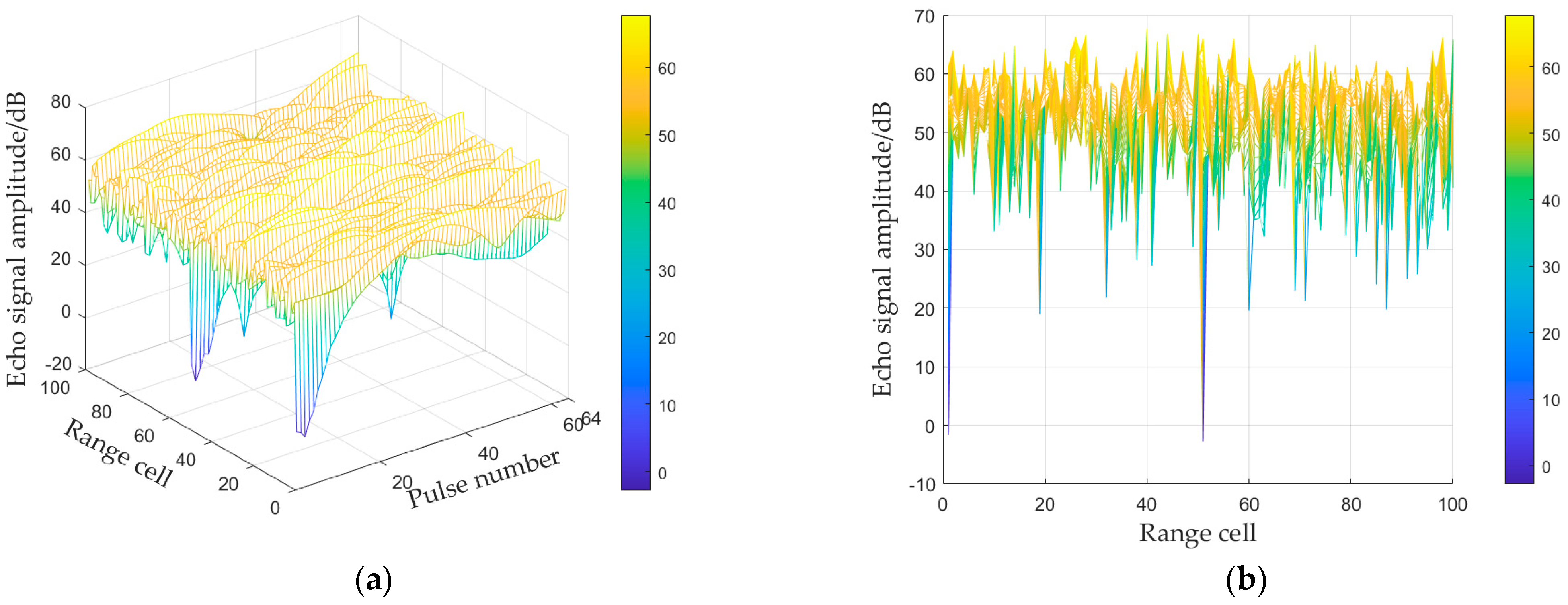
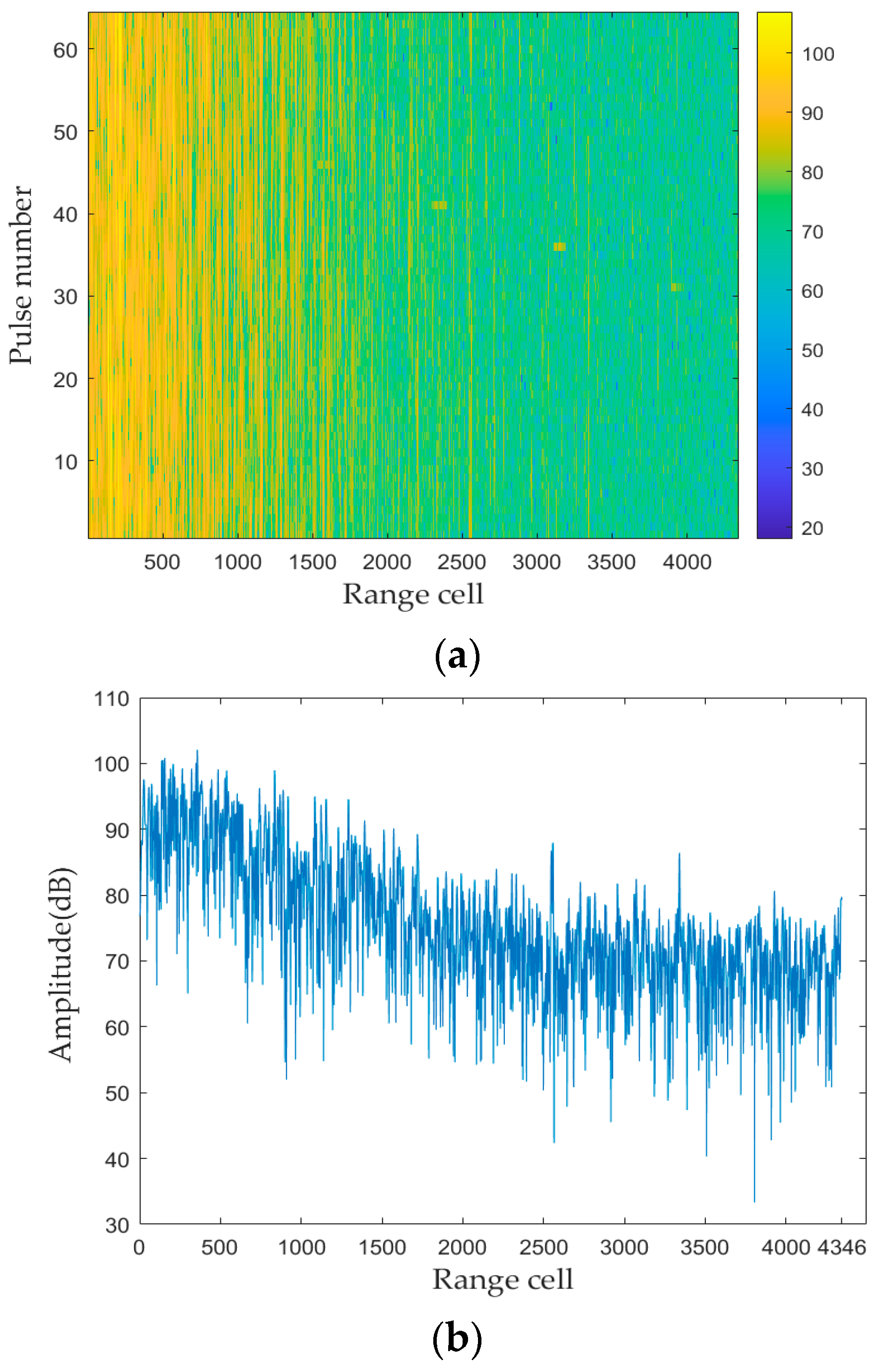
The 2D echo signal and the first pulse echo signal of the radar data are shown in Figure 8. For the 2D echo signal shown in Figure 8, the sea clutter amplitude in this data decreases with the increase in distance, and it can be roughly divided into three clutter regions: Clutter region 1: the first 1000 range cells are the strong sea clutter region, and the average power of the sea clutter is 90.3762 dB. Clutter region 2: 1001~2000 range cells are the clutter–noise mixing region, and the average power is 80.7891 dB. Clutter region 3: 2001~4346 range cells are essentially the noise region, and the average power is 70.974 dB.

Figure 8. Radar echo image before clutter suppression. (a) Two-dimensional echo signal view; (b) range dimension image of the first pulse.

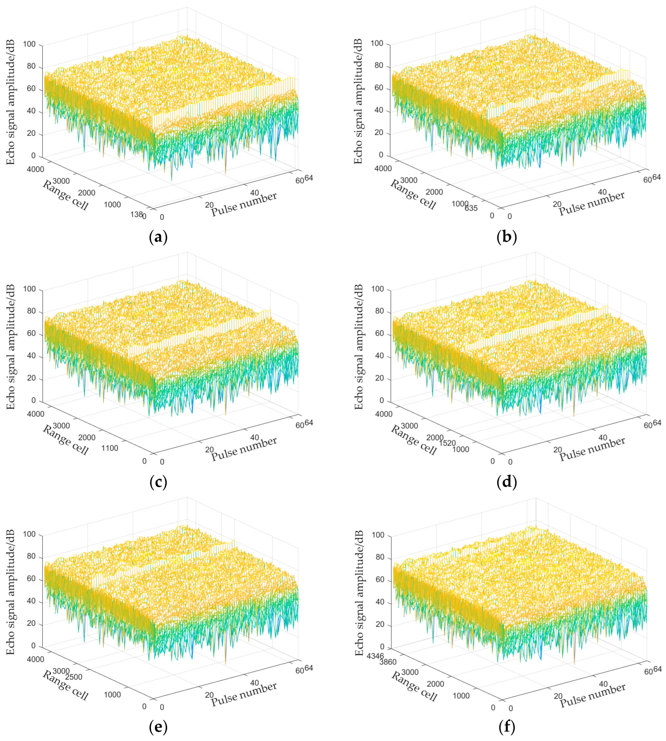
In this section, the experiments will test the clutter suppression effect of the four methods under different clutter intensity regions of the real data and the simulation target with an input SCNR of −10 dB, respectively. The 138th and 635th distance cells are selected to be added to the simulation target in the clutter region 1 where the average power of sea clutter is about 90 dB, the 1100th and 1520th distance cells are selected to be added to the simulation target in the clutter region 2 where the average clutter power is about 80 dB of clutter–noise mixing, and the 2500th and 3860th range cells are selected to be added to the simulation target in the noise region of clutter region 3 with an average power of about 70 dB. A total of six sets of experiments are conducted, and Figure 9 shows the results of the proposed method after clutter suppression.

Figure 9. Three-dimensional view of the proposed method after clutter suppression. (a) The simulation target is located at the 138th range cell. (b) The simulation target is located at the 635th range cell. (c) The simulation target is located at the 1100th range cell. (d) The simulation target is located at the 1520th range cell. (e) The simulation target is located at the 2500th range cell. (f) The simulation target is located at the 3860th range cell.

From Figure 9, it can be seen that the adaptive clutter suppression method based on DRL can still effectively suppress the sea clutter under different clutter intensity environments, but there are some differences in the clutter suppression effect of different range cells. In the strong sea clutter region and the clutter–noise mixing region, the clutter suppression effect is significantly better than in the noise region. This is because the sea clutter energy in clutter region 1 and clutter region 2 is higher than the target energy when the input SCNR is −10 dB, and the sea clutter spectral characteristics are more obvious. After obtaining the estimated clutter spectral center and the spectral width, the agent explores and exploits near the clutter spectral center to optimize the parameter settings of the filters and to change the width of the filters. In the case of minimizing the loss of the target signal, a notch is formed in the center of the clutter, and the sea clutter in that range cell is completely filtered out. Meanwhile, due to the different distribution of sea clutter in each range cell, the exploration and utilization strategies of agents will be different. For example, at range cell 138, the proposed method is able to achieve a higher output SCNR gain with a lower input SCNR. Meanwhile, in the clutter–noise mixing region, where both clutter and noise exist, the spectral analysis of this range cell is more complex, which makes the agent require more frequent and complex adjustments for exploration and exploitation, thus affecting the optimal parameter configuration of the filter. This leads to the difficulty of achieving the same optimization effect for agents in the hybrid noise and clutter region in the same training rounds. In the noise region, the energy is more dispersed, the spectrum of the clutter signal is not concentrated, the energy is low, and the spectral characteristics are not as obvious as in the strong sea clutter region and the clutter–noise mixing region. Moreover, the average clutter power in the noise region is 70.9746 dB, the energy of the clutter signal is lower than that of the target signal, and the spectra of the clutter and the target signal overlap more, so it is difficult to find obvious spectral characteristics to locate the center of the clutter, which leads to the clutter suppression effect not being as effective as in the strong sea clutter region and the clutter–noise mixing region.

Table 8 shows the statistics of SCNR before and after the clutter suppression of each method in different clutter strength environments. It can be seen that the MTI method is effective in different clutter environments, and the output SCNR is stabilized at about 7 dB. The effect of environments with different clutter strengths on the performance of the MTI method is not significant, which is due to the fact that the notch depth of the MTI filter cannot completely suppress the clutter component of this range cell, and there is a certain Doppler shift in the sea clutter, so the suppression effect is limited. The suppression performance of the SVD method shows a decrease in the output SCNR or even an invalid suppression of the clutter as the clutter environment changes. This is because the clutter signal is easily recognized and removed when the power of the clutter signal is much larger than the power of the target signal, so the singular value decomposition (SVD) method effectively separates the clutter signal and suppresses it in clutter region 1. In clutter region 2, the average power of the clutter is about 80 dB, and the energy of the target signal is close to that of the clutter signal, so it is difficult for the SVD method to clearly distinguish between the target signal and the clutter signal during the decomposition, which leads to a decrease in the effect of separating the signal from the clutter. Clutter region 3 is a noise region without obvious sea spikes, and the target signal energy is higher than the clutter energy, the target is mistakenly canceled as sea clutter, and the SVD method is invalid. Compared with the MTI method, the traditional eigenvector method increases the SCNR by about 2 dB in each clutter region, while the proposed method further increases the SCNR by adding a deep Q-network to interact with the environment and continuously learning, which makes the position of the filter notch “more accurate”, “deeper”, and “wider” and further improves the output SCNR to about 15 dB in average. Overall, the proposed method exhibits excellent SCNR in different clutter environments.

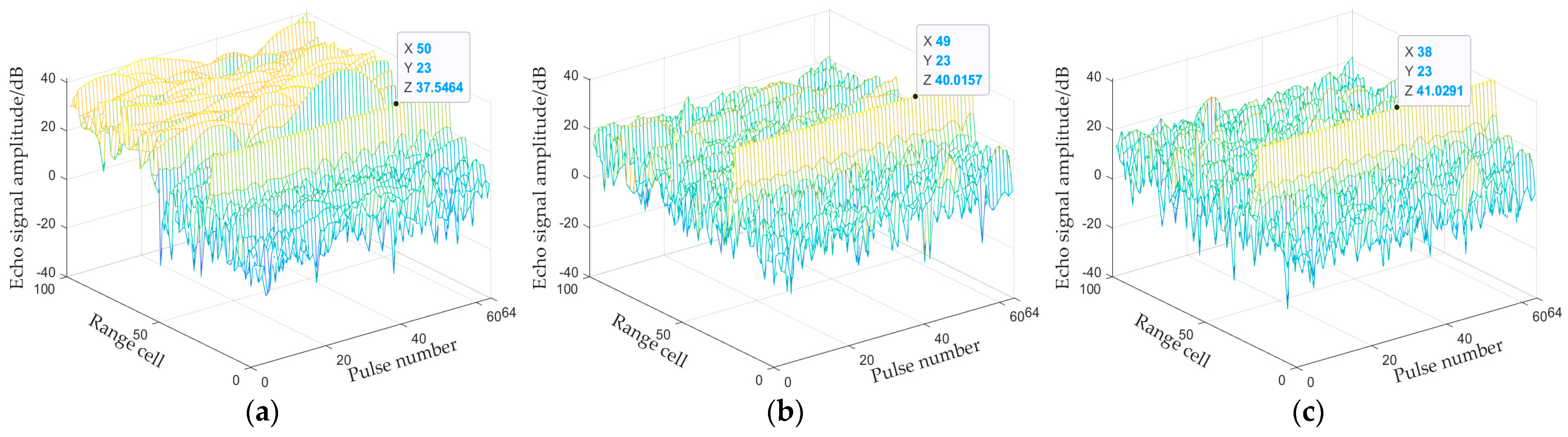
Table 8. Clutter suppression results of each method in different clutter intensity environments.

	Clutter Region 1		Clutter Region 2		Clutter Region 3
Average Clutter Power in Clutter Region	90.3762		80.7891		70.9746
Range cell of target	138	635	1100	1520	1520	3860
MTI method	7.5789	7.1721	7.0347	7.3106	6.9516	7.1702
SVD method	10.2088	8.0744	5.9770	4.2950	Invalid	Invalid
Traditional eigenvector method	8.3439	7.2806	9.1280	9.2615	9.0879	9.8341
Proposed method	16.0097	15.4120	15.8478	15.6033	14.3195	12.6496
Proposed method output SCNR gain	26.0097	25.4120	25.8478	25.6033	24.3195	22.6496

From Figure 4, it can be seen that when the target is located at the 23rd range cell and is in clutter region 1, the clutter center frequency is 0 Hz. At this time, the three-pulse MTI can suppress the clutter in clutter region 1. Since the target’s frequency is located at 440 Hz, which is farther away from the zero frequency, the target is not completely eliminated, but there is a loss of the target signal power, which is 37.5464 dB, and the target signal is reduced by 7.4536 dB. Due to the higher frequency of the clutter in clutter region 2, it can be seen that the clutter in this region is not completely suppressed in Figure 4a, but the clutter is attenuated after the three-pulse canceller. Figure 4b,c show the comparison of the clutter suppression of the traditional eigenvector method and the proposed method. Clutter 1 and 2 regions are suppressed because the two methods produce a depression in the center of the clutter frequency, so as to carry out the suppression of the clutter. The maximum power of the target after the processing of the two methods is 40.0157 dB and 41.0291 dB, respectively, the given target power is 45 dB, and the comparison of the data shows that the loss of target power is minimized after the clutter processing of the proposed method in this paper.

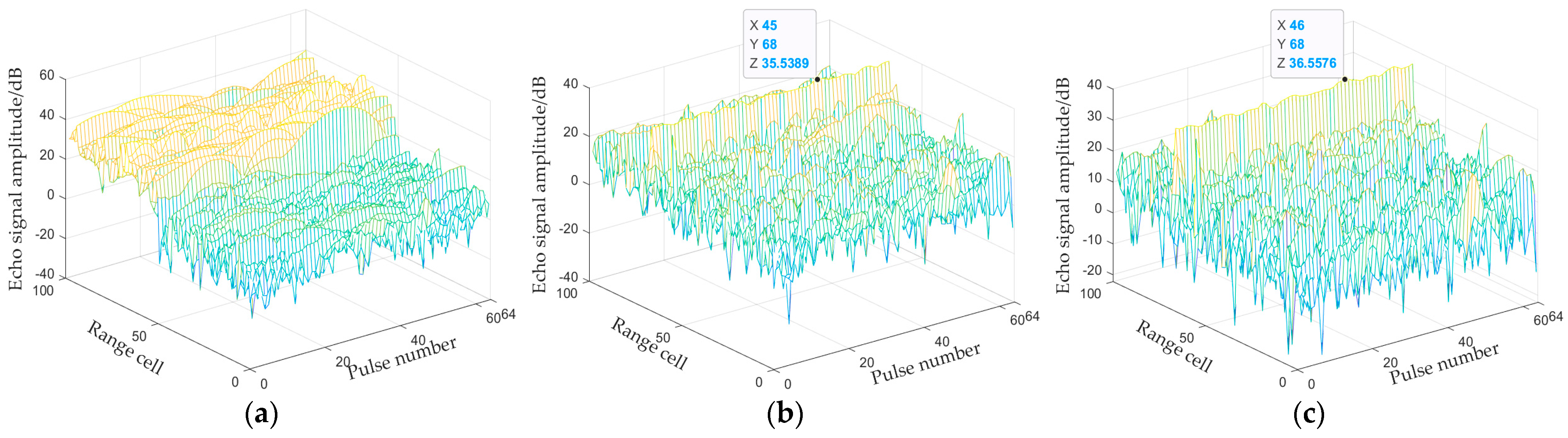
From Figure 5, it can be seen that for the clutter with a certain center frequency, the MTI method cannot effectively suppress the high-frequency clutter, and the target in clutter region 2 is still masked after the MTI three-pulse canceller. While the traditional eigenvector method and the proposed method are still effective in suppressing the clutter to highlight the target, the target signal power is reduced compared to the experimental results of the clutter at 0 center frequency. This is due to the clutter center frequency of clutter region 2 being at 150 Hz. When the feature vector method predicts the clutter center frequency and produces a depression at 150 Hz, while the target is located at 440 Hz, the target frequency is closer to the clutter center frequency, which inevitably attenuates the signal of the neighboring frequency, resulting in a reduction in the target signal power. The maximum power of the target is 35.5389 dB and 36.5576 dB, and the SCNRs are 21.2227 dB and 22.9845 dB, respectively. The filter designed by the proposed method in this paper still outperforms the traditional eigenvector method in clutter region 2.

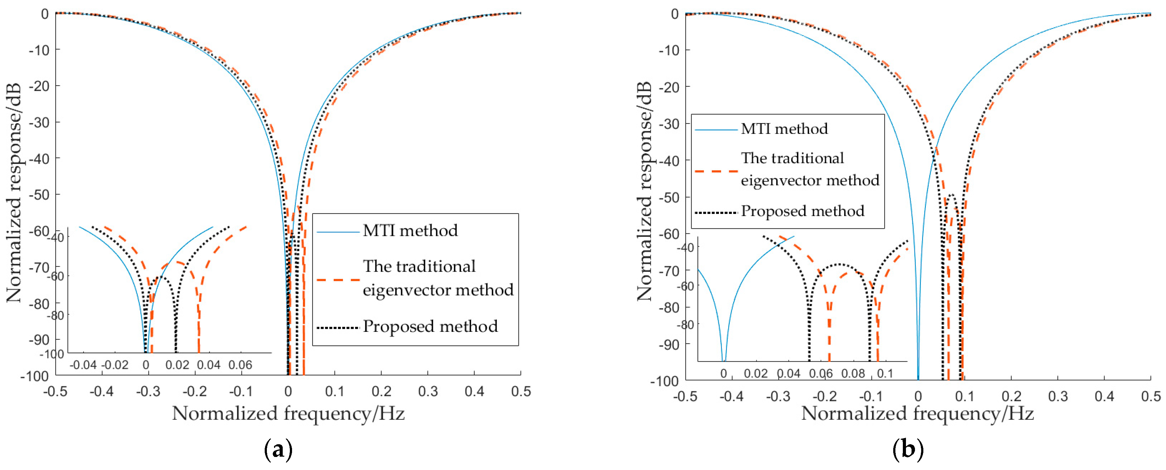
Figure 6a shows the filter response curves of the three methods when the target is located in the 23rd range cell. The MTI three-pulse canceller generates a notch at the zero frequency, and the depth of the notch meets the need for clutter suppression, but the width of its zero-frequency notch is insufficient to completely filter out the clutter. The traditional eigenvector method produces a notch at the center of the corresponding clutter frequency to suppress the clutter under the prediction of clutter information, which can completely filter out the clutter but inevitably loses part of the signal energy. The method proposed in this paper explores and exploits the same predicted clutter spectrum near the center, optimizes the parameter settings of the filter, and changes the filter width. It can be seen that the filter notch designed by the method proposed in this paper is much narrower and is able to completely suppress the clutter while having a higher amplitude-frequency response to signals at non-clutter frequencies, thus reducing the loss of the target signal. In Figure 6b, the conventional eigenvector method produces a notch near 150 Hz, on which the proposed method further optimizes the filter notch width and position to suppress clutter while reducing the target signal loss, while the three-pulse cancellation still produces a notch at the zero frequency, which is unable to suppress the non-zero-frequency clutter.

In conclusion, by analyzing the above four sets of experiments, it can be found that the proposed method in this paper outperforms the MTI three-pulse canceller and the traditional eigenvector method in terms of the combined performance of clutter suppression processing and the degree of target power loss.

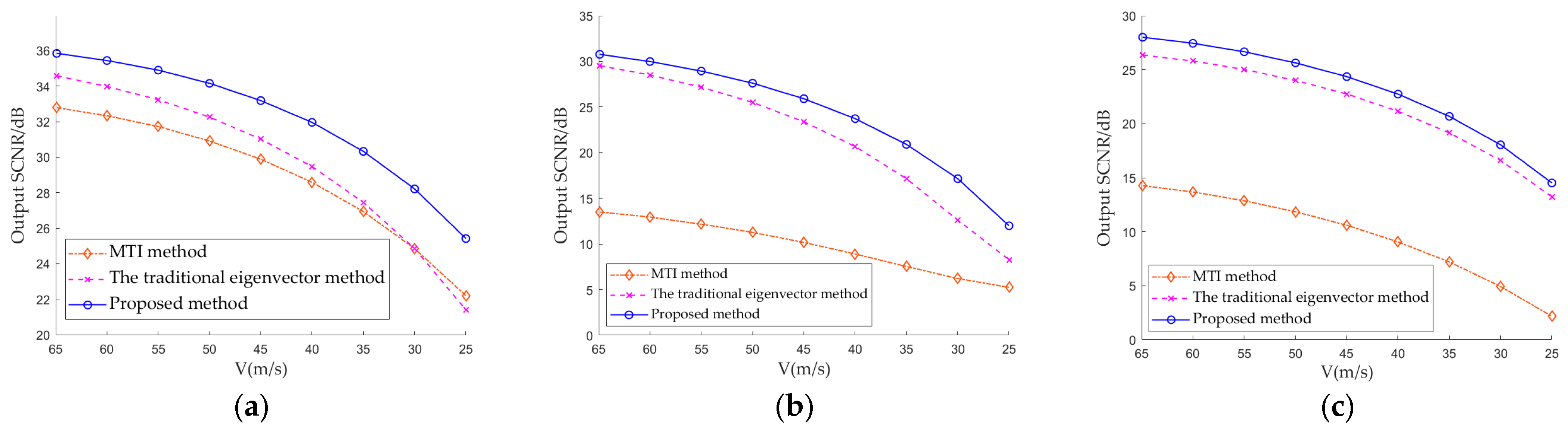
From Figure 7a, it can be seen that when the clutter is located at the zero frequency, the output SCNR of the three methods is significantly improved. As the target speed decreases, the output SCNR gradually decreases, due to the fact that the low-speed target is close to the zero frequency, which overlaps with the clutter frequency resulting in poorer clutter suppression. When the clutter is located at 150 Hz, it can be seen from Figure 7b that the notch generated by the MTI three-pulse canceller at zero frequency cannot completely suppress the clutter at 150 Hz, but the clutter is attenuated. In contrast, the traditional eigenvector method and the proposed method in this paper can move the notch of the filter to 150 Hz and suppress the clutter completely. As the speed decreases and the Doppler frequency of the target is close to 150 Hz, the clutter suppression effect of the two methods deteriorates, but the adaptive clutter intelligent suppression method based on DRL can still suppress the clutter while minimizing the loss of the target signal, and its output signal heterodyne noise is still higher than that of the traditional eigenvector method. When there are two clutter center frequencies of clutter at the same time, the suppression effects of the three methods are shown in Figure 7c, the MTI three-pulse method does not work for the non-zero-frequency clutter, and it still plays the role of clutter attenuation. Meanwhile, the traditional eigenvector method and the method proposed in this paper can generate double notches in the frequency domain according to the spectral centers of different clutter and generate notches at −150 Hz and 150 Hz at the same time, both of which can completely suppress the clutter, but the filter designed by the method proposed in this paper has a higher output SCNR and a lower loss of target power compared to the filter designed by the traditional eigenvector method.

In conclusion, the adaptive clutter intelligent suppression method based on DRL shows higher output SCNR and lower target power loss under different target speeds and different clutter frequencies, which proves its superior performance and strong adaptive ability in complex environments. In addition, through the dynamic adjustment and optimization of the filter parameters, the method can effectively respond to environmental changes, avoid the performance degradation caused by the complexity and uncertainty of the environment, and improve the stability of the system.

6. Conclusions

In the complex clutter background, the clutter center frequency is not fixed, and the spectral width is large, which leads to the performance degradation of the traditional adaptive clutter suppression method. To address the above problems, this paper proposes an intelligent clutter suppression method based on deep reinforcement learning (DRL). By constructing a filter parameter decision model of the deep Q-network (DQN), establishing a reward and punishment mechanism, and introducing a greedy strategy, the agent continuously interacts with the environment and uses the learning results to optimize the filter parameters in real time, so that the filter’s notch can be “more accurate”, “deeper”, and “wider” to adapt to different clutter strength environments. The experimental results show that the proposed algorithm can still effectively adapt to different clutter strength environments in the complex clutter background, thus significantly improving the clutter suppression effect, and the performance is better in the strong clutter.

Based on the research in this paper, future work will focus on further optimizing the compensation of the blind speed phenomenon. Specifically, we plan to introduce variable pulse repetition frequency (PRF) as an optimization method to address the impact of the blind speed phenomenon on the clutter suppression algorithm. By dynamically adjusting the pulse repetition frequency, we hope to be able to better adapt to changes in the target speed, thereby improving the adaptability and accuracy of the algorithm in complex environments.

In addition, it is worth pointing out that the clutter simulation data in this paper are modeled based on the parameters of the phased-array radar, and the corresponding experimental radar parameters also rely on the phased-array radar. The clutter suppression method is mainly applied to phased array radar and has a strong application background. However, our results are also generalizable, and it is expected that the method can be effectively applied to mechanically scanned radars and other types of radars. Regarding the adaptation to these radar systems, further testing and validation are required in future work. This will be an important direction for our further research.

References

- Borge, J.C.N.; Rodriguez, G.R.; Hessner, K. Inversion of Marine Radar Images for Surface Wave Analysis. J. Atmos. Ocean. Technol. 2004, 21, 1291–1300. [Google Scholar] [CrossRef]
- Barrick, D.E.; Headrick, J.M.; Bogle, R.W.; Crombie, D.D. Sea backscatter at HF: Interpretation and utilization of the echo. Proc. IEEE 1974, 62, 673–680. [Google Scholar] [CrossRef]
- Lipa, B.J.; Barrick, D.E. Extraction of sea state from HF radar sea echo: Mathematical theory and modeling. Radio Sci. 1986, 21, 81–100. [Google Scholar] [CrossRef]
- Ward, K.D.; Watts, S. Use of sea clutter models in radar design and development. IET Radar Sonar Navig. 2010, 4, 146–157. [Google Scholar] [CrossRef]
- Huang, Y.; Chen, X.L.; Guan, J. Property analysis and suppression method of real measured sea spikes. J. Radars 2015, 4, 334–342. [Google Scholar]
- Conte, E.; Lops, M.; Ricci, G. Asymptotically optimum radar detection in compound-Gaussian clutter. IEEE Trans. Aerosp. Electron. Syst. 1995, 31, 617–625. [Google Scholar] [CrossRef]
- Wang, G.; Xia, X.G.; Root, B.T.; Chen, V.; Zhang, Y.; Amin, M. Manoeuvring target detection in over-the-horizon radar using adaptive clutter rejection and adaptive chirplet transform. IEE Proc. Radar Sonar Navig. 2003, 150, 292–298. [Google Scholar] [CrossRef]
- Wei, N.; Li, X.; Li, T.C. An eigenvalue decomposition based method for suppressing multi-mode clutter. J. Radio Sci. 2016, 31, 85–90. [Google Scholar]
- Guan, Z.W.; Chen, J.W.; Bao, Z. A modified adaptive sea clutter suppression algorithm based on PSNR-HOSVD for skywave OTHR. J. Electron. Inf. Techn. 2019, 41, 1743–1750. [Google Scholar]
- Dong, Z.W.; Sun, J.; Sun, J.M. Marine weak moving target detection based on sparse dictionary learning. Syst. Eng. Electron. 2020, 42, 30–36. [Google Scholar]
- Lv, M.; Zhou, C. Study on Sea Clutter Suppression Methods Based on a Realistic Radar Dataset. Remote Sens. 2019, 11, 2721. [Google Scholar] [CrossRef]
- Zhou, Q.; Zheng, H.; Wu, X. Fractional Fourier Transform-Based Radio Frequency Interference Suppression for High-Frequency Surface Wave Radar. Remote Sens. 2020, 12, 75. [Google Scholar] [CrossRef]
- Chen, Z.; He, C.; Zhao, C.; Fei, X. Using SVD-FRFT Filtering to Suppress First-Order Sea Clutter in HFSWR. IEEE Geosci. Remote Sens. Lett. 2017, 14, 1076–1080. [Google Scholar] [CrossRef]
- Shi, Y.L.; Wang, L.; Li, J.H. CFAR detection for small targets on sea surface based on singular value decomposition in project space. Syst. Eng. Electron. 2022, 44, 512–519. [Google Scholar]
- Root, B.T. HF-over-the-horizon radar ship detection with short dwells using clutter cancelation. Radio Sci. 1998, 33, 1095–1111. [Google Scholar] [CrossRef]
- Root, B. HF radar ship detection through clutter cancellation. In Proceedings of the National Radar Conference, Dallas, TX, USA, 14 May 1998; pp. 281–286. [Google Scholar]
- Lee, M.J.; Lee, S.J.; Ryu, B.H. Reduction of False Alarm Rate in SAR-MTI Based on Weighted Kurtosis. IEEE Trans. Geosci. Remote Sens. 2021, 59, 3122–3135. [Google Scholar] [CrossRef]
- Schleher, D.C. MTI and Pulsed Doppler Radar with MATLAB; Artech House: Norwood, MA, USA, 2010. [Google Scholar]
- Sun, G.Z.; Bian, L.X. The technology of radar adaptive clutter suppression. Radar Ecm 2011, 31, 11–13+33. [Google Scholar]
- Li, S.; Chen, Y.J.; Jiang, J. Performance comparison of radar adaptive moving target indication filters. Ship Electron. Eng. 2023, 43, 77–83. [Google Scholar]
- Ding, H.; Dong, Y.L.; Liu, N.B. Overview and prospects of research on sea clutter property cognition. J. Radars 2016, 5, 499–516. [Google Scholar]
- Tang, X.H.; Li, D.; Su, J. An adaptive clutter intelligent suppression method based on AlexNet. J. Signal Process. 2020, 36, 2032–2042. [Google Scholar]
- Fan, Y.F.; Li, C.X.; Li, D.T. A Novel Sea Clutter Suppression Method based on Neural Network. In Proceedings of the 2021 IEEE 4th International Conference on Electronic Information and Communication Technology (ICEICT), Xi’an, China, 18–20 August 2021; pp. 437–440. [Google Scholar]
- Ge, F.X.; Meng, D.H.; Peng, Y.N. Clutter central frequency and bandwidth estimation methods. J. Tsinghua Univ. 2002, 42, 941–944. [Google Scholar]
- Dayan, P.; Daw, N.D. Decision theory, reinforcement learning, and the brain. Cogn. Affect. Behav. Neurosci. 2008, 8, 429–453. [Google Scholar] [CrossRef] [PubMed]
- Liu, Z.Y.; Mu, C.X.; Sun, C.Y. An overview on algorithms and applications of deep reinforcement learning. Chin. J. Intell. Sci. Technol. 2020, 2, 314–326. [Google Scholar]
- Liu, N.B.; Ding, H.; Huang, Y. Annual progress of the sea-detecting X-band radar and data acquisition program. J. Radars 2021, 10, 173–182. [Google Scholar]
- Liu, N.B.; Dong, Y.L.; Wang, G.Q. Sea-detecting X-band radar and data acquisition program. J. Radars 2019, 8, 656–667. [Google Scholar]