Optimized Discrete Nonlinear Control of Alternating Current Three-Phase Motors via an Industrial Variable Frequency Drive

Abstract

This article presents a suboptimal nonlinear control strategy to improve the dynamics of a three-phase alternating current (AC) motor. Using dynamic programming, the calculation of the Bellman function is avoided by determining a suboptimal control sequence that locally minimizes a quadratic performance index at each step. The motor’s fixed-frame nonlinear mathematical model controls the stator currents, rotor magnetic fluxes, and rotor angular speed by applying voltages to the stator. Experimental tests are conducted using a Delta VFD007EL11A variable frequency drive (VFD), demonstrating improved motor state behavior and performance compared to an optimal proportional integral (PI) control and a fixed reference input in the VFD. The experiments include set point changes and a comparative analysis of the energy consumption between both controllers considering two cases: free and with load on the motor shaft.

1. Introduction

Modern motor control methods are those that provide the power supply to the motor through a power converter that allows for the regulation of the supplied voltage and frequency. Induction motors can be viewed as complex nonlinear control systems, and there are mainly three control strategies: scalar control or V/F control, where the manipulated variables are the magnitude and frequency of each voltage or current supplied to the stator; the field oriented control (FOC), which allows one to regulate the electromagnetic torque generated by the motor; and modern control, which regulates all the states of the nonlinear or linear plant [1].

Some examples of scalar control applied to induction motors include ref. [2], where the control was implemented on the Compact RIO control board 9074, which was used along with a static frequency converter to supply the three-phase asynchronous motor with a squirrel cage rotor. Additionally, a fuzzy logic controller was developed in LabVIEW software for speed regulation, and its performance was compared to the speed control with a PI control. In ref. [3], simulations and experimental results were provided by applying a dual-mode adaptive robust controller to control the angular shaft speed of a three-phase induction motor. A microcomputer received the rotor speed using a tachometer, and Hall effect sensors were used to measure the currents of two phases of the motor. In ref. [4], LabVIEW software: https://studyatncepu.ncepu.edu.cn/docs/2023-12/d52f7540704649bdb7a1929e989190bd.pdf, accessed on 8 April 2024 running on a field programmable gate array, was used to design a V/F control. A general purpose inverter controller was used to control the speed of the induction motor with a pulse width modulation technique. MATLAB/Simulink, https://studyatncepu.ncepu.edu.cn/docs/2023-12/d52f7540704649bdb7a1929e989190bd.pdf, accessed on 8 April 2024 and LabVIEW tools were used for the simulations and experiments.

With respect to the field oriented control (FOC), in ref. [5], an adaptive indirect FOC based on a rotor flux observer was presented. Rotor flux estimation was based on the backstepping technique using the integral of tracking errors. It was implemented in real time using a dSPACE DS1104R&D board with a TMS320F240 digital signal processor and ControlDesk software: https://www.sciencedirect.com/science/article/abs/pii/S0888327017303801, accessed on 6 February 2024 for the control of the load torque and rotor speed of the 3 kW induction motor. In ref. [6], motor speed control via the FOC approach was synthesized, and constant flux control of a three-phase induction motor was calculated. It was performed using the discrete linearized three input–three output model (stator angular frequency, two components of the stator space voltage vector–rotor angular speed, and two components of the stator space flux linkage). Furthermore, a robust optimal preview control was proposed. The simulation and experimental results were presented using a dSpace DS 1104 control board.

Focusing on the developed advanced modern control techniques for three-phase induction motors, in some works, including ref. [7], a quasi-linearization approach was presented that converts the nonlinear optimal control problem of a three-phase induction motor (modeled as a third order nonlinear model) into a sequence of linear quadratic optimal control problems. The simulation results are presented. In ref. [8], the predictive control model approach was applied to the induction motor drive system that controls its torque and current. Using the linear state-space representation (currents were state variables), the simulation results were shown. In ref. [9], the implementation of an optimal control based on quadratic criteria was presented in a low-power electric drive with a three-phase induction motor. The dSPACE 1104 controller was used to obtain the optimal online solution of the Riccati matrix differential equation. A linear model was considered, and its state variables were the rotor speed and the angular position of the rotor field. Based on the optimal solution and the corresponding feedback signals, the optimal speed reference for the AC drive system was obtained and tracked by the Altivar 71 inverter. It was compared with the inner rotor field oriented control and the PI controller of the Altivar 71 inverter. Experimental results of speed and load torque regulation were presented. In ref. [10], a robust adaptive speed position tracking control was presented for a mathematical model of the linear fith-order induction motor mathematical model with unknown end effects and secondary resistance.

Other works related to the synthesis of advanced control strategies considering the full state (fifth-order) nonlinear model of the induction motor have been developed. For example, in ref. [11], a nonlinear predictive control was synthesized to regulate an induction motor in a water pumping system. This scheme was validated via simulations. Another similar work on predictive control is ref. [12], as well as applications of motor control such as ref. [13]. In ref. [14], a discrete-time sliding mode control of an induction motor was designed to regulate the rotor speed and stator current. Real-time experiments were carried out using a dSpace system with the DS1104 control board based on the TMS320F240 digital signal processor. In ref. [15], an indirect rotor flux oriented control and backstepping control of a five-phase induction motor drive were presented. The performance of both controllers was analyzed through experimental validation.

Most of the synthesized control strategies in the specialized literature were validated via simulation results [7,11] or by experiments using a test bench [2,3,4,5,6,10,14,15] without the use of an industrial inverter. In fact, there are few projects that use industrial VFDs that incorporate advanced control techniques [9], possibly because industrial VFDs generally have a closed architecture. For instance, in ref. [16], a remote control system for an induction motor was presented using a PLC OMRON CJ1M- CPU11-ETN21 (Kyoto, Japan) and LabVIEW software. A VFD OMRON SYSDRIVE 3G3MV-A2007 was used to change the speed control. The whole system was in an open loop since there was no practical data measurement from the actual output of the motor. In ref. [17], the VFD Altivar 71 was preconfigured to accept speed reference via the Modbus communication protocol from a Raspberry Pi board; however, there was no closed-loop system, and neither control strategy was mentioned. In ref. [18], an induction motor (three-phase, 380 V, 50 Hz, four-pole, low-voltage squirrel cage) drove a conveyor belt for a bottle filling plant. The open loop control of motor speed and direction control was performed using data sent through a PLC (Schneider Electric Modicon TM241CEC24R (Rueil-Malmaison, France)) connected for serial communication (RS485 port) to the VFD (ATV12H075M2), whose parameters (speed, direction, acceleration, and deceleration) were changed and monitored using the Modbus protocol to communicate with a SCADA server.

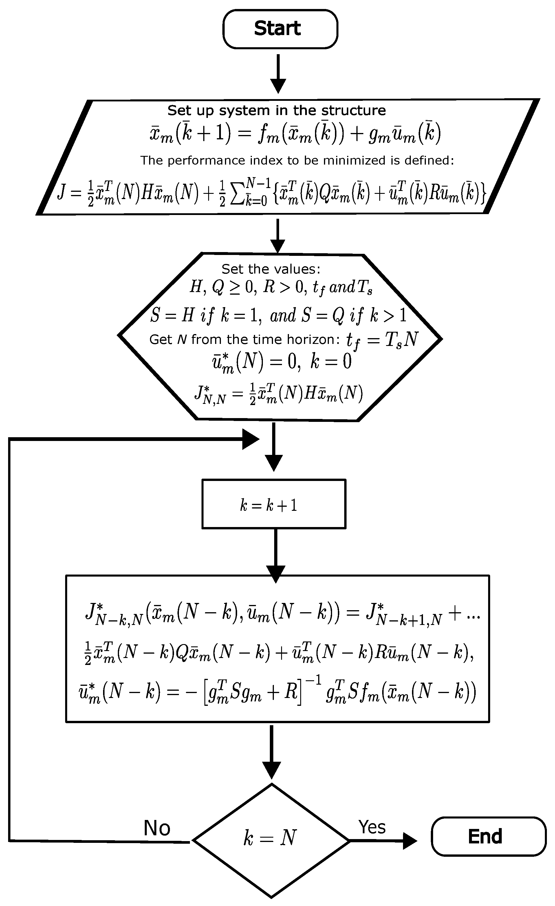
The dynamic programming approach was used as a base to develop the nonlinear control for the Baldor IDNM3534 induction motor, which was modeled using the Clarke transformation from three phases into two phases [1], leading to an equivalent representation given by an affine nonlinear fifth-order model. The main ideas of the dynamic programming approach exposed here were originally proposed in ref. [19]. This approach was applied to the unmanned aerial vehicle (UAV) in ref. [20], an autonomous soaring UAV in ref. [21], to a hybrid exoskeleton in ref. [22], and a tomato dehydrator modeled as discrete affine nonlinear systems with delayed input [23].

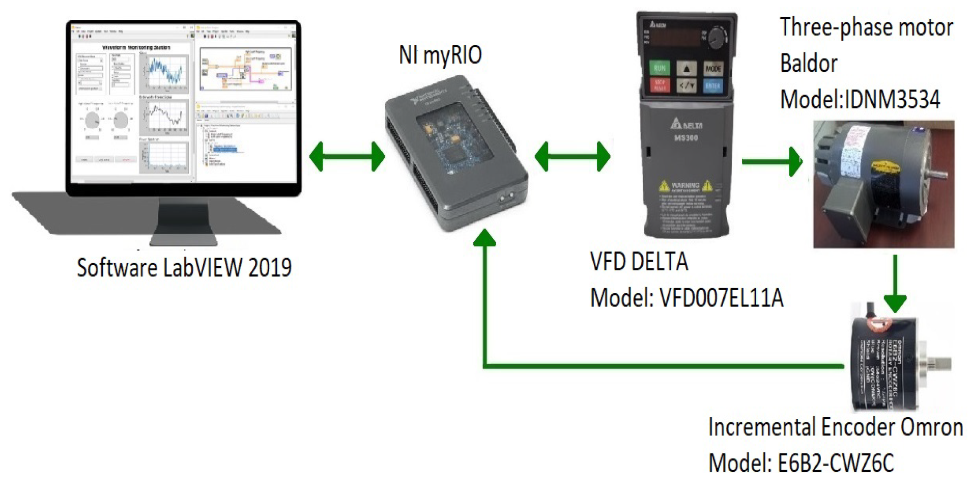
Since the rotor flux is not usually measurable, in some cases, it is obtained via an observer. However, in this proposal, the real-time reconstruction of the fluxes is carried out according to ref. [24]; that is, using measured variables and the mathematical model. These flux estimations, the stator currents (obtained from an industrial VFD Delta VFD007EL11A), and the rotor speed (measured from an encoder) are used for the computation of the proposed nonlinear discrete suboptimal control, which uses the plant model. The real-time experiments are made using a data acquisition NI MyRIO card, an industrial VFD, and LabVIEW software, in which a command interface is developed to set the setpoints (experimentally obtained), the penalty matrices for computation of the discrete suboptimal controller, and the nonlinear control strategy. The inner PID control of an industrial VFD, usually used to regulate the velocity of the rotor of the motor, is tuned (the proportional part is the unity, the integral and derivative parts are disabled) to allow the external control signal from the MyRIO card and the PC with LabVIEW software. The setpoint of the inner PID of the VFD is set to zero using the potentiometer available from the VFD. The internal PID control of the VFD is configured with positive feedback (the part of the process variable is positive and configured as an analog input of the VFD). In this analog input, the suboptimal nonlinear control signal, given by the MyRIO card (a root mean square voltage that is proportional to frequency, which guarantees the relation of V/F of the VFD) is introduced to the industrial VFD instead of the encoder signal. The encoder signal is read through the MyRIO card and processed using LabVIEW software. A comparison with an optimal PI controller using the VI LabVIEW PID of the Control toolkit is made.

The main contributions of the paper are summarized as follows:

• The experimental application of the discrete suboptimal controller for the nonlinear induction motor model is developed with a relatively low cost to regulate the five state variables of the biphasic system.
• An industrial VFD is used as interface between the nonlinear control and the AC motor by using a MyRIO card and LabVIEW software. The experiments were conducted with different sampling times.
• The real-time reconstruction of the rotor fluxes is obtained directly from the nonlinear model and is used to calculate the suboptimal nonlinear discrete control.
• Good tracking performance and robustness to unknown parameters is obtained when the set point is varying (without and with load on the motor shaft). The proposed suboptimal nonlinear discrete controller improves the operation of the V/F scalar control (currents and fluxes tracking) of the industrial VFD when compared with an optimal PI. It gives experimental evidence that the mathematical model used is a good approximation of the real behavior of the AC motor.

This paper is organized as follows. Section 2 is devoted to useful results for the implementation of the proposed scheme. In Section 3, the suboptimal sequence to regulate a transformed biphasic system is synthesized. The experimental results are presented in Section 4, and finally, in Section 5, concluding comments are presented.

2. Preliminares

2.1. Induction Motor Mathematical Model

The stator windings of electrical machines with AC are intended to generate a sinusoidally distributed conductor density, so the distributed density in the air gap will be sinusoidal. Considering a squirrel-cage rotor, the density in the bars is uniform; however, the currents present in the same bars produce a magnetomotive force (mmf), which is sinusoidally distributed, allowing, it to replace the stator and rotor windings of the induction motor, respectively, with an equivalent of sinusoidally distributed balanced three-phase windings [25,26].

To obtain the mathematical model considered, we consider the following assumptions.

• Magnetic circuits are linear and three-phase windings are balanced.
• The magnetic material in the stator and rotor operates in its linear region, and it has a very high value for the permeability factor; saturation, iron losses, end-windings, and slot-effects are ignored.
• The machine is symmetric.
• The stator resistance is constant.

According to these assumptions, based on the general equations that describe the mathematical model of the three-phase motor [27] (pp. 135, 170), [26], the Clarke transform is applied to convert from a three-phase system to a two-phase system, obtaining as a result a fifth-order model that describes the dynamics of a balanced induction motor. This model is expressed in a fixed reference frame attached to the stator $(a,b)$ [26] and is given as follows:

$${\displaystyle \frac{d\omega }{dt}}=\mu ({\psi }_{ra}{i}_{sb}-{\psi }_{rb}{i}_{sa})-{\displaystyle \frac{T_L}{J}},$$

$${\displaystyle \frac{d{\psi }_{ra}}{dt}}=-\alpha {\psi }_{ra}-\omega {\psi }_{rb}+\alpha L_m{i}_{sa},$$

$${\displaystyle \frac{d{\psi }_{rb}}{dt}}=-\alpha {\psi }_{rb}+\omega {\psi }_{ra}+\alpha L_m{i}_{sb},$$

$${\displaystyle \frac{d{i}_{sa}}{dt}}=-\gamma i_{sa}+{\displaystyle \frac{v_{sa}}{\sigma }}+\beta \alpha {\psi }_{ra}+\beta \omega {\psi }_{rb},$$

$${\displaystyle \frac{d{i}_{sb}}{dt}}=-\gamma i_{sb}+{\displaystyle \frac{v_{sb}}{\sigma }}+\beta \alpha {\psi }_{rb}-\beta \omega {\psi }_{ra},$$

(1)

where $\sigma =L_s-{\displaystyle \frac{{L_m}^2}{L_r}},$ $\beta ={\displaystyle \frac{L_m}{\sigma L_r}},$ $\gamma ={\displaystyle \frac{R_s}{\sigma }}+\beta \alpha L_m,$ $\alpha ={\displaystyle \frac{R_r}{L_r}},$ $\mu ={\displaystyle \frac{L_m}{J{L}_r}},$ $T_L$ is the load torque, $R_s$ and $R_r$, are the resistances of the stator and rotor, $L_s$ and $L_r$ the self-inductances of the stator and rotor, and $L_m$ is the mutual inductance. The state variables $[\omega ,{\psi }_{ra},{\psi }_{rb},i_{sa}$, and $i_{sb}]$ denote the speed of the rotor, the components of the rotor flux, and the rotor current, respectively, and the input variables $v_{sa},v_{sb}$ are the voltage input to the machine. The Clarke inverse transformation [26] is applied to obtain the three-phase signal in AC, then this signal is converted to a root mean square voltage, which is equivalent to the calculated control signal for each phase. Then, it is adjusted with a proportionality constant to maintain the V/F relation according to the characteristics of VFD Delta VFD007EL11A [28]. Although the VFD Delta VFD007EL11A cannot directly control the motor torque, the scalar control tries to maintain the maximum torque available based on the V/F relation [28].

2.2. Flux Reconstruction

If one wants to use modern control to synthesize the controls $v_{sa}$ and $v_{sb}$ to regulate all the states $[\omega ,{\psi }_{ra},{\psi }_{rb},i_{sa},i_{sb}],$ then the knowledge of all these state variables must be available. In this work, measurements of the speed rotor $\omega \left(t\right)$ (given by an incremental encoder) and $I_{sa}$ of the three-phase system (its root mean square value is given by the industrial VFD) are available. It is important to mention that the currents $i_{sa}$ and $i_{sb}$ are obtained via the Clarke transformation using the current $I_{sa}$. $I_{sb}$ and $I_{sc}$ are assumed to have the same magnitude as $I_{sa}$ with a phase change. Furthermore, since the motor is controlled without load torque, $T_L$ could be considered zero. However, measurements of the fluxes ${\psi }_{ra}\left(t\right)$ and ${\psi }_{rb}\left(t\right)$ are not available. Then, the reconstruction of the rotor fluxes is based on the estimation of the electrical parameters of the motor, the currents $i_{sa}$ and $i_{sb}$, and the angular velocity $\omega$. Consequently, a state observer is not necessary. Starting from the model (1), the fluxes can be expressed as the sum of the voltage vectors, current vectors, and current derivatives [24] from the fourth and fifth equations. After direct manipulations of these equations, we obtain the following expressions:

$$\left[\begin{array}{c}{\psi }_{ra}\left(t\right)\\ {\psi }_{rb}\left(t\right)\end{array}\right]={\displaystyle \frac{1}{\beta ({\alpha }^2+{\omega }^2)}}\left[\begin{array}{cc}\alpha & -\omega \\ \omega & \alpha \end{array}\right]\left[\begin{array}{c}{\displaystyle \frac{d{i}_{sa}}{dt}}+\gamma i_{sa}-{\displaystyle \frac{v_{sa}}{\sigma }}\\ {\displaystyle \frac{d{i}_{sb}}{dt}}+\gamma i_{sb}-{\displaystyle \frac{v_{sb}}{\sigma }}\end{array}\right].$$

(2)

In these expressions, the fluxes are a function of the available variables.

As is well known, the approximation must depend mainly on the structure and parameters of the model [29].

Here, the parameters of the mathematical model corresponding to the induction motor are identified by the recursive least squares matrix inverse (RLS) algorithm [30,31] due to its simplicity, which requires a relatively low computational cost. Furthermore, in ref. [32], the authors mentioned the feasibility of combining the optimal control approach with the RLS algorithm.

This algorithm was implemented using LabVIEW software, and the estimated parameters are used to synthesize the nonlinear control. This is described in the following section.

3. Suboptimally Controlled Induction Motor

This section is devoted to showing the application of the dynamic programming approach to synthesize suboptimal nonlinear control for an induction motor.

3.1. Discrete Model

The nonlinear model given by (1) is discretized using a Euler approximation. The uniform sampling time is defined as $T_s$ and $t=k{T}_s$, where $k=0,1,2,\dots ,N$. The dynamics of the state vector of the model given by (1) are approximated as follows:

$${\displaystyle \frac{d}{dt}}\left[\begin{array}{c}\omega \left(t\right)\\ {\psi }_{ra}\left(t\right)\\ {\psi }_{rb}\left(t\right)\\ i_{sa}\left(t\right)\\ i_{sb}\left(t\right)\end{array}\right]\approx {\displaystyle \frac{1}{T_s}}\left[\begin{array}{c}\omega (k+1)-\omega \left(k\right)\\ {\psi }_{ra}(k+1)-{\psi }_{ra}\left(k\right)\\ {\psi }_{rb}(k+1)-{\psi }_{rb}\left(k\right)\\ i_{sa}(k+1)-i_{sa}\left(k\right)\\ i_{sb}(k+1)-i_{sb}\left(k\right)\end{array}\right]$$

(3)

Then, the discretized nonlinear model given by (1) is expressed as follows:

$${\overline{x}}_m(k+1)=f_m\left({\overline{x}}_m\left(k\right)\right)+g_m{\overline{u}}_m\left(k\right),$$

(4)

where

$${\overline{x}}_m\left(k\right)={\left[\begin{array}{ccccc}\omega \left(k\right)& {\psi }_{ra}\left(k\right)& {\psi }_{rb}\left(k\right)& i_{sa}\left(k\right)& i_{sb}\left(k\right)\end{array}\right]}^T,$$

$$f_m\left({\overline{x}}_m\left(k\right)\right)=$$

$$\left[\begin{array}{c}\omega \left(k\right)+T_s\left[\mu ({\psi }_{ra}\left(k\right)i_{sb}\left(k\right)-{\psi }_{rb}\left(k\right)i_{sa}\left(k\right))\right]\\ (1-T_s\alpha ){\psi }_{ra}\left(k\right)-T_s\omega \left(k\right){\psi }_{rb}\left(k\right)+T_s\alpha L_m{i}_{sa}\left(k\right)\\ (1-T_s\alpha ){\psi }_{rb}\left(k\right)+T_s\omega \left(k\right){\psi }_{ra}\left(k\right)+T_s\alpha L_m{i}_{sb}\left(k\right)\\ (1-T_s\gamma )i_{sa}\left(k\right)+T_s\beta \alpha {\psi }_{ra}\left(k\right)+T_s\beta \omega \left(k\right){\psi }_{rb}\left(k\right)\\ (1-T_s\gamma )i_{sb}\left(k\right)+T_s\beta \alpha {\psi }_{rb}\left(k\right)+T_s\beta \omega \left(k\right){\psi }_{ra}\left(k\right)\end{array}\right],$$

$$f_m\left({\overline{x}}_m\left(k\right)\right)=\left[\begin{array}{c}{f}_1\left({\overline{x}}_m\left(k\right)\right)\\ f_2\left({\overline{x}}_m\left(k\right)\right)\\ f_3\left({\overline{x}}_m\left(k\right)\right)\\ f_4\left({\overline{x}}_m\left(k\right)\right)\\ f_5\left({\overline{x}}_m\left(k\right)\right)\end{array}\right],$$

(5)

$$g_m={\left[\begin{array}{ccccc}0& 0& 0& {\displaystyle \frac{T_s}{\sigma }}& 0\\ 0& 0& 0& 0& {\displaystyle \frac{T_s}{\sigma }}\end{array}\right]}^T,$$

(6)

and

$${\overline{u}}_m\left(k\right)={\left[\begin{array}{cc}{v}_{sa}\left(k\right)& v_{sb}\left(k\right)\end{array}\right]}^T.$$

The sampling time $T_s$ is adjusted to 1 ms (experiments without a load), 100 µs, and 50 µs (test with a load).

3.2. Synthesis of the Suboptimal Control for the AC Motor

In order to obtain the suboptimal control that regulates the discrete state ${\overline{x}}_m\left(k\right)$ of the nonlinear discrete system (4), first observe that the nonlinear map $f_m(.)$ is well defined with respect to its arguments. The origin is a fixed point of the system given by (4), which means $f_m\left(0\right)=0$ when the control vector ${\overline{u}}_m\left(k\right)\in {\mathbb{R}}^2$ is equal to zero and $k=0,1,\dots ,N$ for some $N\in \mathbb{N}$.

Consider the following definition about controllability for discrete systems.

Definition 1.

The pair $({\overline{x}}_{m0},{\overline{x}}_{m1})$ is controllable if there exists an admissible control sequence ${\overline{u}}_m\left(k\right)$ such that the system defined by (4) is transferred from ${\overline{x}}_{m0}$ to ${\overline{x}}_{m1}$ in N finite number of steps.

It is not difficult to demonstrate that the system given by (4) is locally controllable. In fact, one can linearize the system given by (4) around the fixed point zero and verify that the linear discrete system is controllable. Therefore, the system given by (4) is controllable according to Definition 1, at least in the local sense (see, for example, ref. [8]).

The main ideas of the dynamic programming approach exposed in the following were originally exposed in ref. [19]. Here, the algorithm is adapted to be applied to regulate all the states of the nonlinear model given by (4). Next, the performance index is defined as a quadratic form to be locally minimized with respect to the control sequence ${\overline{u}}_m\left(k\right)$ subject to the trajectories of the system given by (4). In fact, the following quadratic index is considered:

$$J={\displaystyle \frac{1}{2}}{\overline{x}}_m^T\left(N\right)H{\overline{x}}_m\left(N\right)+{\displaystyle \frac{1}{2}}\sum _{k=0}^{N-1}\left\{{\overline{x}}_m^T\left(k\right)Q{\overline{x}}_m\left(k\right)+{\overline{u}}_m^T\left(k\right)R{\overline{u}}_m\left(k\right)\right\},$$

(7)

where $H, Q\ge 0$ and $R>0$ are square matrices of appropriate dimensions, and $t_f=T_{s}N$ defines the horizon. As in the linear quadratic regulator (LQR), matrices H and Q penalize the state convergence, and R penalizes the energy applied to the system.

The optimization problem could be established as follows:

Problema 1.

To find a suboptimal sequence ${\overline{u}}_m\left(k\right)$ that minimizes (in the local sense) to the performance index given by (7), along the trajectories of the system given by (4).

The problem of finding a global optimal control sequence that minimizes the performance index given by (7) involves the solution of the Hamilto–Jacobi–Bellman (HJB) equation in its discrete version. However, finding the solution of the HJB equation for nonlinear systems represents a very difficult problem [32].

The following proposition gives a solution to Problem 1.

Proposition 1.

Consider the system given by (4) and the quadratic performance index given by (7). A suboptimal sequence ${\overline{u}}_m\left(k\right)$, which causes the performance index (7) to reach a minimum in the local sense, is described by the following entries:

$$\begin{array}{c}{v}_{sa}^{\ast }(N-k)=-\sigma T_s\left({\displaystyle \frac{f_1\left({\tilde{x}}_m(N-k)\right)s_{41}+f_2\left({\tilde{x}}_m(N-k)\right)s_{42}+f_4\left({\tilde{x}}_m(N-k)\right)s_{44}}{r_{11}{\sigma }^2+s_{44}{T}_s^2}}\right),\\ v_{sb}^{\ast }(N-k)=-\sigma T_s\left({\displaystyle \frac{f_1\left({\tilde{x}}_m(N-k)\right)s_{51}+f_2\left({\tilde{x}}_m(N-k)\right)s_{52}+f_5\left({\tilde{x}}_m(N-k)\right)s_{55}}{r_{22}{\sigma }^2+s_{55}{T}_s^2}}\right),\end{array}$$

(8)

where $s_{ij}=h_{ij}$ if $k=1$, $s_{ij}=q_{ij}$ if $k=2,\dots ,N$, and the matrices H, Q, and R are given as follows:

$$H=\left[\begin{array}{ccccc}{h}_{11}& 0& 0& h_{14}& h_{15}\\ 0& h_{22}& 0& h_{24}& h_{25}\\ 0& 0& h_{33}& 0& 0\\ h_{41}& h_{42}& 0& h_{44}& 0\\ h_{51}& h_{52}& 0& 0& h_{55},\end{array}\right],$$

$$Q=\left[\begin{array}{ccccc}{q}_{11}& 0& 0& q_{14}& q_{15}\\ 0& q_{22}& 0& q_{24}& q_{25}\\ 0& 0& q_{33}& 0& 0\\ q_{41}& q_{42}& 0& q_{44}& 0\\ q_{51}& q_{52}& 0& 0& q_{55}\end{array}\right],$$

(9)

and

$$R=\left[\begin{array}{cc}{r}_{11}& 0\\ 0& r_{22}\end{array}\right].$$

(10)

The entries of the matrices are such that H and Q are symmetric positive semidefinite matrices, and R is a symmetric positive definite matrix.

Proof. 

The proof is based on the dynamic programming approach and is given in the Appendix A. □

Remark 1.

These particular structures of the three matrices, H, Q, and R, guarantee that the controllers $v_{sa}^{\ast }$ and $v_{sb}^{\ast }$ involve all the state variables of ${\overline{x}}_m$.

Remark 2.

According to the proof of Proposition 1 given in Appendix A, the procedure exposed there avoids the solution of the HJB equation by using sufficient conditions of the optimality on the variational calculus approach [33].

Figure 1 shows the flow diagram that summarizes the proposed control.

Both controllers $v_{sa}^{\ast }$ and $v_{sb}^{\ast }$ are constructed considering errors, which means ${\tilde{x}}_m\left(k\right)={\overline{x}}_m\left(k\right)-{\overline{x}}_{m,ss}\left(k\right)$, where ${\overline{x}}_{m,ss}\left(k\right)$ is the desired state. Stable state values are experimentally obtained for both controllers and set points (${\overline{x}}_{m,ss}\left(k\right)$) for state variables. The fluxes are estimated using the formula given in (2) in its discretized version using the Euler approximation for the derivatives of $i_{sa}$ and $i_{sb}$. The controllers given by (8) are programmed in the LabVIEW software. The details of their implementation are given in the following section.

4. Experimental Results

4.1. Global Architecture Scheme

The control loop consists of a PC with LabVIEW software, a MyRIO acquisition card, an AC three-phase motor Baldor IDN M3534, St. Louis, MI, USA, an incremental encoder E6B2-CWZ6C, an industrial VFD Delta VFD007EL11A, and a switch S202-K4 ABB.

Table 1. Parameters of the AC motor Baldor. Source: Baldor Electric Company (St. Louis, MO, USA) [34].

CAT NO	IDNM3534
FRAME	56C
Rated Output (HP)	0.33
Volts	230/460
Full Load Amps	1.1/0.55
R.P.M.	1750
Hz	60
Phase	3

and

Table 2. Parameters of the VFD Delta. Source: Delta Electronics, INC [28].

MODEL:	VFD007EL11A
INPUT	1 PH 100–120 V 50/60 Hz
OUTPUT	3 PH 0–240 V 4.2 A 0.75 kW/1 HP
FREQUENCY RANGE	0.1–600 Hz

describe the main characteristic parameters of the AC motor and the Delta industrial VFD, respectively.

Figure 2 displays the interconnection between the devices.

4.2. Implementation of the Suboptimal Control

This section describes how signal processing was performed to implement suboptimal control. Figure 3 illustrates the proposed scheme. The following is the proposed implementation method:

(1) The off-line part consists of considering the general equations rewritten by the Clarke transform and subsequently its discretization. Finally, the recursive least squares method exposed in Section 2.2 is applied to identify the parameters of the discretized nonlinear system.

(2) In the online part of the proposed scheme, which uses the dynamic programming approach in the discrete time domain considering a quadratic performance index, a suboptimal finite-horizon control sequence is obtained using the algorithm presented in Section 3.2. Applying the inverse Clarke transform, it is possible to return to a three-phase system, and since the system is balanced, only one phase of it is considered. For the said phase (stator voltage), its effective value (RMS) is calculated, and based on the operating principle of the scalar control system, the conversion to a frequency reference signal (control signal) is performed. This control signal is sent through the myRIO board to the VFD. The system feedback is the rotor speed measured through an incremental encoder and the stator current provided by the VFD. Both signals are connected to the myRIO board (see Figure 3).

Figure 4 shows the proposed control scheme.

It could be described as follows. The inner PID control of an industrial VFD, usually used to regulate the velocity of the rotor of the motor, is tuned as follows: the proportional part is the unity, and the integral and derivative parts are disabled (parameters 10.02, 10.03, and 10.04 in the VFD, respectively, see

Table 3. VFD Delta VFD007EL11A parameters.

Parameter	Explanation	Setting
01.09	Acceleration time 1 (s)	0.1
01.10	Deceleration time 1 (s)	0.1
02.00	Source of first master frequency command	4
02.01	Source of first operation command	0
02.02	Stop method	1
03.03	Analog output signal selection	1
10.00	PID set point selection	1
10.01	Input terminal for PID feedback	0
10.02	Proportional gain (P)	1
10.03	Integral time (I)	0.00
10.04	Derivative control (D)	0.00
10.19	PID calculation mode selection	1

). It allows an external control signal to enter to the VFD from the MyRIO card and the PC with the LabVIEW software. The setpoint of the inner PID of the VFD is set to zero by the VFD menu configuration by setting the available knob to the dispositive. The inner PID comparator of the VFD is configured with positive feedback: The part of the process variable is positive. In the only analog input available in the VFD, the suboptimal nonlinear control signal, given by the MyRIO card, is introduced. A root mean square voltage, which is equivalent to the calculated voltage for each phase, is introduced to the industrial VFD in the input terminal for the PID feedback of the VFD. The encoder signal is read through the MyRIO card and processed in LabVIEW software. To evaluate the efficiency of the proposed controller, the acceleration and deceleration times are adjusted to the minimum value available in the VFD. A parallel configuration of the inner PID was programmed in the VFD. The adjustment of the VFD Delta VFD007EL11A parameters is shown in Table 3.

It is important to clarify that the set points for each tested operation zone were obtained via a previous step response experiment, and they are taken as the stable state values of each state variable. The stable state values are calculated for the controllers and depend on the values of the system parameters and the setpoints. These stable state values of $v_{sa}$ and $v_{sb}$ are added to the suboptimal controllers given by (8).

Despite the fact that the control loop does not have torque feedback, the torque given by the motor is maximized by the frequency inverter using the V/F control approach of the VFD [28].

4.3. Real Time Experiments Using Nonlinear Discrete Control and Optimal PI Control

Three experiments were conducted using the inner PID of the industrial VFD configured with the proportional gain as one and the integral and derivative parts set to zero:

(1) The suboptimal nonlinear discrete control signal plus offset was sent to the VFD using an analog input and the software LabVIEW (without and with a load).

(2) An optimal PI control was implemented using the virtual instrument PID of LabVIEW, and its control signal was sent to the VFD via an analog input without and with a load.

(3) A constant signal was introduced to the industrial VFD. This constant represents the RMS voltage in a stable state (the offset of the first experiment described here) to maintain the velocity of the motor shaft at a specific setpoint.

First, all experiments were carried out without a load on the shaft, and we selected four different setpoints: 800 RPM, 600 RPM, 400 RPM, and 300 RPM. These setpoint changes were made to test the performance of both controllers in different operating zones and to observe possible overshoots and undershoots in each change and the settling time of the process variable.

Table 4. Set points (SP) and stable state values for the controllers without a load.

SP (Rotor Speed)	SP Stator Current (${\mathit{I}}_{\mathit{sa}}$, Three-Phase System)	SP Flux (${\mathbf{\Psi }}_{\mathit{ra}}$, Three-Phase System)	Stable State Stator Voltage (${\mathit{V}}_{\mathit{sa}}$, Three-Phase System)
800 RPM	0.78 A	0.013 Wb	97.5 ${\mathrm{VAC}}_{r}ms$
600 RPM	0.81 A	0.019 Wb	73.2 ${\mathrm{VAC}}_{r}ms$
400 RPM	0.82 A	0.028 Wb	49 ${\mathrm{VAC}}_{r}ms$
200 RPM	0.85 A	0.059 Wb	24 ${\mathrm{VAC}}_{r}ms$

shows the setpoint values used in the experiments and the stable-state stator voltage for each setpoint of the rotor speed.

The horizon of the performance index given by (7) was fixed at $N=\mathrm{140,000}$, which corresponds to a time of 140 s, with a sampling time of 0.001 s. The following numerical values were chosen for the matrices Q, H, and R:

$$H=\left[\begin{array}{ccccc}10& 0& 0& 3& 1\\ 0& 10& 0& 1& 1\\ 0& 0& 10& 0& 0\\ 3& 1& 0& 10& 0\\ 1& 1& 0& 0& 10,\end{array}\right],$$

$$Q=\left[\begin{array}{ccccc}10& 0& 0& 1& 1\\ 0& 10& 0& 1& 1\\ 0& 0& 10& 0& 0\\ 1& 1& 0& 10& 0\\ 1& 1& 0& 0& 10\end{array}\right],$$

and

$$R=\left[\begin{array}{cc}0.009& 0\\ 0& 0.009\end{array}\right].$$

(11)

A profile of the rotor speed was previously established and is shown in Figure 5. To compare the performance of the controllers given by (8), an optimal PI was implemented (see ref. [35]) considering a first-order plant for each set point of the rotor speed. Based on this strategy, the penalization matrices $Q_{He}$ and $R_{He}$ were chosen according to the desired performance of the system response (for some maximum overshoot and settling time). The gains obtained were introduced into the PID block function of the LabVIEW software. These gains were $K_p=0.1$ and $K_i=0.08$.

Figure 5 shows the response of the rotor speed when both schemes (suboptimal nonlinear control and optimal PI) were used. A smooth response can be seen when the suboptimal nonlinear control was used: no overshoot was shown, and both controllers displayed an undershoot when the rotor speed setpoint was lower in the time instants of 20, 40, and 60 s. The undershoot can be explained, because the motor does not have a break system. However, the suboptimal control presents less undershoot compared to the optimal PI.

Figure 6 shows the control signal $V_{sa}$ calculated using the LabVIEW software and sent to the VFD. A smoother control signal can be seen when the suboptimal nonlinear control is applied; this implies a behavior with fewer oscillations in the rotor speed (see Figure 5).

Figure 7 depicts the error signal of the rotor speed. A light advantage of the suboptimal nonlinear control can be seen; this advantage is greater with the changes in the setpoint.

Figure 8 shows the tracking of the stator current $I_{sa}$ given for the VFD. A clear advantage can be observed when using the suboptimal nonlinear control. In fact, the convergence of all state variables to the set points is better, in the sense that they do not present large oscillations. This implies energy savings, resulting in less deterioration of the rotor windings [36].

The estimated flux ${\Psi }_{ra}$ of the three-phase system is shown in Figure 9. Similar to the stator current $I_{sa}$, a significant advantage is shown when the suboptimal control is used compared to the optimal PI control. On the one hand, notice that if an overflux occurs, it may cause saturation of the magnetic core of the stator and rotor. Saturation causes overheating and can lead to motor failure [37]. On the other hand, when the magnetic flux is reduced, it reduces the torque capability and affects the motor’s ability to handle the load [36].

Finally, another experiment without a load is conducted. In fact, the stable-state voltage for each setpoint of rotor speed is introduced in the analog input of the VFD via the software LabVIEW and the MyRIO card, which means that the scheme is in am “open loop”. However, the industrial VFD has an inner V/F control. The results of this comparison with respect to the rotor speed are shown in Figure 10. Clearly, the suboptimal control outweighs the “open loop” signal.

Figure 11 shows the stator current for the three-phase system. Clearly, the initial transitory peak of the current is greater than the one produced by the suboptimal control and the optimal PI.

Figure 12 shows the flux for the three-phase system. Important variations occur when the “open loop” signal is applied, in contrast to the suboptimal control, which is smoother.

Remark 3.

The use of modern control along with industrial VFDs for AC motors is not common in the specialized literature (please see the cited references in the Introduction). Due to the good performance of the proposed control scheme, this could be a potential complement to a variable frequency driver (VFD) with inner V/F control, which allows for suboptimal regulation of the all states (currents, fluxes, and angular velocity), which is not possible with the PID available in the industrial VFDs.

Table 5. Overshoot, undershoot, and settling time for each of the setpoints: 800 RPM, 600 RPM, 400 RPM, and 200 RPM.

Operation Region	Controller	${\mathit{M}}_{\mathit{p}}$/${\mathit{U}}_{\mathit{s}}$ (%)	${\mathit{T}}_{\mathit{s}}$ (s)
800 RPM	Suboptimal	−/−	1.41
	Optimal PI	$5.00$/−	1.71
600 RPM	Suboptimal	−/$0.83$	0.6
	Optimal PI	−/$4.33$	1.1
400 RPM	Suboptimal	−/$2.00$	0.7
	Optimal PI	−/$6.75$	1.3
200 RPM	Suboptimal	−/−	0.5
	Optimal PI	−/$11.75$	1.0
400 RPM	Suboptimal	−/−	0.9
	Optimal PI	$5.5$/−	1.3
600 RPM	Suboptimal	−/−	0.6
	Optimal PI	$3.3$/−	1.2
800 RPM	Suboptimal	−/−	0.5
	Optimal PI	$3.12$/−	1.3

compares the overshoot ($M_p$), undershoot ($U_s$), and the settlement time for the setpoints of 800 RPM, 600 RPM, and 400 RPM between both controllers, the suboptimal nonlinear discrete control and optimal PI control, in the time interval [0, 80] corresponding to decreasing set points and (80, 140] corresponding to increasing set points of the programmed trajectory tracking task.

According to the results given in Table 5, the suboptimal discrete nonlinear control (SDNC) provides a better performance compared to the optimal PI (OPI). This is because SDNC does not produce overshoots, and it presents a response with lower undershoots than those produced by OPI.

Table 6. IAE of $\omega$, $I_{sa}$, and ${\Psi }_{ra}$: energy consumption.

Controller	IAE $\mathit{\omega }$	IAE ${\mathit{I}}_{\mathit{sa}}$	IAE ${\mathbf{\Psi }}_{\mathit{ra}}$	Energy (Wh)
Suboptimal	13.37	8.85	7.50	2.08
Optimal PI	15.47	30.91	46.85	2.12

shows the integral absolute errors (IAE) of the angular velocity of the motor shaft ($\omega$), the stator current ($I_{sa}$), and the rotor flux (${\Psi }_{ra}$). The energy consumption is calculated based on the current measurements $I_{sa}$ and the voltage $V_{sa}$ during all the experiments and is shown in Table 6.

The experiments described in this section were carried out on a three-phase motor with a free load and a sampling time of 1 ms. In the next section, load experiments are presented. In these new tests, the sampling time is fixed to 50 µs and 100 µs to guarantee precise sampling of the measurements.

4.4. Real-Time Experiments Using a Load on the AC Motor

In this section, load experiments are presented considering a 5.25 kg metallic piece on the motor shaft. Both controllers are used to conduct the experiments. Figure 13a shows the metal piece. The metallic piece coupled to the motor shaft is shown in Figure 13b.

Figure 14 shows the angular velocity when a load is coupled to the motor shaft. When the loaded motor shaft is at rest and a set point of 400 RPM is requested, the optimal PI response presents an important overshoot, in contrast to non-linear suboptimal control.

Figure 15 shows the error of the angular velocity for both controllers when a load on the motor shaft is considered.

Figure 16 shows the currents for both controllers when a load is considered in the motor shaft.

An important overshoot of current is seen when the motor is in rest and starts the motor shaft spin. Figure 17 shows the estimate of the flux rotor for both controllers when a load is considered.

The calculated control signals are shown in Figure 18.

In general, the control signal presents higher energy consumption when an optimal PI is used.

Table 7. Overshoot, undershoot, and settling time for each of the setpoints: 400 RPM and 200 RPM. (Sampling time: 50 µs).

Operation Region	Controller	${\mathit{M}}_{\mathit{p}}$/${\mathit{U}}_{\mathit{s}}$ (%)	${\mathit{T}}_{\mathit{s}}$ (s)
400 RPM	Suboptimal	−/−	3.9
	Optimal PI	$47.25$/−	4.1
200 RPM	Suboptimal	−/−	1.1
	Optimal PI	$11.5$/13	2.7
400 RPM	Suboptimal	−/−	0.6
	Optimal PI	$8.92$/−	1.8
200 RPM	Suboptimal	−/−	0.5
	Optimal PI	$17.9$/$14.3$	3.3

shows the performance comparison of both controllers when a sampling time of 50 µs is considered.

Table 8. IAE of $\omega$, $I_{sa}$, and ${\Psi }_{ra}$: energy consumption (sampling time: 50 µs).

Controller	IAE $\mathit{\omega }$	IAE ${\mathit{I}}_{\mathit{sa}}$	IAE ${\mathbf{\Psi }}_{\mathit{ra}}$	Energy (Wh)
Suboptimal	12,239.85	68.36	1.95	0.72
Optimal PI	14,158.27	141.38	16.74	0.99

shows the integral absolute errors (IAE) of the angular velocity of the motor shaft ($\omega$), the stator current ($I_{sa}$), and the rotor flux (${\Psi }_{ra}$). The energy consumption is calculated based on the current measurements $I_{sa}$ and the voltage $V_{sa}$ during all experiments.

Figure 19 shows the angular velocity when a sampling time of 100 µs and a load of 5.25 kg are considered.

A clear advantage can be appreciate when the SNDC is used. Figure 20 shows the error of the angular velocity for both controllers. The error is greater when there is a change in the set point.

Figure 21 shows the currents for both controllers when a load is considered in the motor shaft.

Again, an overshoot of the current in the beginning of the experiment can be observed. Figure 22 shows the estimate of the flux rotor for both controllers when a load is considered, with a sampling time of 100 µs.

The calculated control signals are shown in Figure 23 when a load in the motor shaft is considered.

The control signal corresponding to the SNDC is softer when it is compared with the control signal of the OPI.

Table 9. Overshoot, undershoot, and settling time for each of the setpoints: 400 RPM and 200 RPM. (Sampling time: 100 µs).

Operation Region	Controller	${\mathit{M}}_{\mathit{p}}$/${\mathit{U}}_{\mathit{s}}$ (%)	${\mathit{T}}_{\mathit{s}}$ (s)
400 RPM	Suboptimal	−/−	4.33
	Optimal PI	$48.8$/−	4.4
200 RPM	Suboptimal	−/$4.65$	1.4
	Optimal PI	$29.7$/14	3
400 RPM	Suboptimal	−/−	1.7
	Optimal PI	$7.32$/−	2.1
200 RPM	Suboptimal	−/$5.45$	0.6
	Optimal PI	$18.15$/$10.15$	3.4

shows the performance comparison of both controllers when a sampling time of 100 µs is considered.

Table 10. IAE of $\omega$, $I_{sa}$, and ${\Psi }_{ra}$: energy consumption (sampling time: 100 µs).

Controller	IAE $\mathit{\omega }$	IAE ${\mathit{I}}_{\mathit{sa}}$	IAE ${\mathbf{\Psi }}_{\mathit{ra}}$	Energy (Wh)
Suboptimal	13,900.54	68.66	1.78	1.25
Optimal PI	17,199.96	138.98	15.73	1.667

shows the integral absolute errors (IAE) of the angular velocity of the motor shaft ($\omega$), the stator current ($I_{sa}$), and the rotor flux (${\Psi }_{ra}$). The energy consumption is calculated based on the current measurements $I_{sa}$ and the voltage $V_{sa}$ during all the experiments.

The SNDC performs better across all state variables and with respect to energy consumption than the OPI control when a load is considered in the motor shaft.

Remark 4.

Some possible error sources on the implementation of proposed scheme are as follows:

On the one hand, the choice of the H, Q, and R matrices and the correct estimation of the plant parameters are crucial issues to obtain a good performance of the closed-loop system. On the other hand, mechanical vibration sources should be avoided. It is advisable that the load has a uniform mass distribution and a correct coupling to the motor shaft to obtain good measurements of the encoder dispositive. Mechanical vibration produces errors in the measurements and estimation of state variables.

5. Conclusions

Based on the dynamic programming approach, a suboptimal nonlinear sequence was synthesized and experimentally applied (without and with a load on the motor shaft) to an induction motor using a Delta industrial VFD VFD007EL11A. The proposed control scheme improves the performance of the inner V/F control of the VFD when the proposed control is compared to an optimal PI controller and a fixed external signal. A good performance of the suboptimal nonlinear discrete control is exhibited, and the five state variables of the transformed system are regulated. The advantages of SNDC extend to energy consumption, even when a load on the shaft is considered. The dimensionality issue of the dynamic programming approach is avoided by finding a local minimum on each step. Then, the proposed scheme is liable to being implemented in a low-cost digital system because it requires a relatively low memory space and its structure involves simple arithmetic operations. The suboptimal nonlinear control uses a nonlinear model of the three-phase motor, and it allows for a better performance of the controlled variables (fluxes, currents, and angular velocity of the motor shaft) on a wide operation zone, in contrast with previous results that use a linear model of the plant. Some factors that influence the effectiveness of the proposed algorithm in improving motor performance are the following: The proposed control is an optimized controller, and this implies a relative low energy consumption and consequently a smooth response of the controlled variables, with an adequate selection of the penalty matrices $Q, H$, and R. The use of an industrial-grade VFD guarantees adequate behavior of the regulated variables, together with the proposed control scheme. Finally, an adequate parameter identification model allows for the correct performance of the proposed control, which is synthesized via the mathematical model. In fact, the comparative analysis made in the previous section provides experimental evidence of the effectiveness of the proposal, despite the presence of a load on the motor shaft. Future work includes the implementation of the optimal vector control to compare with the suboptimal control.

References

1. Marino, R.; Tomei, P.; Verrelli, C.M. Induction Motor Control Design; Springer Science & Business Media: Greer, SC, USA, 2010. [Google Scholar]
2. Livinti, P. Speed control of the asynchronous motor using LabVIEW. Int. J. Adv. Appl. Sci. 2021, 8, 59–66. [Google Scholar] [CrossRef]
3. Cunha, C.D.; Araujo, A.D.; Barbalho, D.S.; Mota, F.C. A dual-mode adaptive robust controller applied to the speed control of a three-phase induction motor. Asian J. Control 2005, 7, 197–201. [Google Scholar] [CrossRef]
4. Ahmed, A.; Shaikh, A.M.; Shaikh, M.F.; Shaikh, S.A.; Soomro, J.B. Experimental Study of Various Parameters during Speed Control of Three-phase Induction Motor Using GPIC and LabVIEW. Ann. Emerg. Technol. Comput. 2021, 5, 51–62. [Google Scholar] [CrossRef]
5. Regaya, C.B.; Farhani, F.; Zaafouri, A.; Chaari, A. A novel adaptive control method for induction motor based on Backstepping approach using dSpace DS 1104 control board. Mech. Syst. Signal Process. 2018, 100, 466–481. [Google Scholar] [CrossRef]
6. Negm, M.M.; Bakhashwain, J.M.; Shwehdi, M.H. Speed control of a three-phase induction motor based on robust optimal preview control theory. IEEE Trans. Energy Convers. 2006, 21, 77–84. [Google Scholar] [CrossRef]
7. Tamimi, J.; Jaddu, J. Nonlinear optimal controller of three-phase induction motor using quasilinearization. In Proceedings of the Second International Symposium on Communications, Control and Signal Processing, Marrakech, Morroco, 13–15 March 2006. [Google Scholar]
8. Farah, N.; Talib, H.N.; Ibrahim, Z.; Abdullah, Q. Analysis and investigationof different advanced control strategies for high-performance induction motor drives. Telkomnika 2020, 18, 3303–3314. [Google Scholar] [CrossRef]
9. Gaiceanu, M.; Rosu, E.; Munteanu, T.; Dumitriu, T.; Paduraru, R.; Dache, C. Optimal control for AC drive with quadratic criteria. In Proceedings of the IEEE 2009 13th European Conference on Power Electronics and Applications, Barcelona, Spain, 8–10 September 2009; pp. 1–10. [Google Scholar]
10. Lian, K.Y.; Hung, C.Y.; Chiu, C.S.; Fu, L.C. Robust adaptive control of linear induction motors with unknown end-effect and secondary resistance. IEEE Trans. Energy Convers. 2008, 23, 412–422. [Google Scholar] [CrossRef]
11. Massaq, Z.; Abounada, A.; Mohamed, R. Robust non-linear control of a hybrid water pumping system based on induction motor. Int. J. Power Electron. Drive Syst. 2020, 11, 1995–2006. [Google Scholar] [CrossRef]
12. Kawai, H.; Zhang, Z.; Kennel, R.; Doki, S. Direct speed control based on finite control set model predictive control with voltage smoother. IEEE Trans. Ind. Electron. 2022, 70, 2363–2372. [Google Scholar] [CrossRef]
13. Liu, C.; Yao, J.; Jia, Y. Vehicle height control based on active suspension with permanent magnet synchronous linear motor. Proc. Inst. Mech. Eng. Part D J. Automob. Eng. 2024, 238, 1191–1200. [Google Scholar] [CrossRef]
14. Chihi, A.; Azza, H.B.; Jemli, M.; Sellami, A. Nonlinear discrete-time integral sliding mode control of an induction motor: Real-time implementation. Stud. Inform. Control 2017, 26, 23–32. [Google Scholar] [CrossRef]
15. Echeikh, H.; Trabelsi, R.; Iqbal, A.; Bianchi, N.; Mimouni, M.F. Comparative study between the rotor flux oriented control and non-linear backstepping control of a five-phase induction motor drive—An experimental validation. IET Power Electron. 2016, 9, 2510–2521. [Google Scholar] [CrossRef]
16. Barsoum, N.; Chin, P.R. Ethernet control AC motor via PLC using LabVIEW. J. Intell. Control Autom. 2011, 2, 330–339. [Google Scholar] [CrossRef]
17. Filipović, F.; Petronijevixcx, M.; Mitrovixcx, N.; Bankovixcx, B. Affordable Virtual Laboratory for Remote Control of Variable Speed Drives. In Proceedings of the 52nd International Scientific Conference on Information, Communication and Energy Systems and Technologies (ICEST), Niš, Serbia, 28–30 June 2017; pp. 354–357. [Google Scholar]
18. Engin, D.; Engin, M.; Pınar, S.; Candan, M. PLC and SCADA Based Real-Time Monitoring and Control of Networked Processes. J. Multidiscip. Eng. Sci. Technol. 2021, 8, 14070–14080. [Google Scholar]
19. Kirk, D.E. Optimal Control Theory: An Introduction, Dever Books on Electricarl Engineering Series; Dover Publications: New York, NY, USA, 2004. [Google Scholar]
20. Santos-Sánchez, O.; García, O.; Romero, H.; Salazar, S.; Lozano, R. Finite horizon nonlinear optimal control for a quadrotor: Experimental results. Optim. Control Appl. Methods 2021, 42, 54–80. [Google Scholar] [CrossRef]
21. Ángeles-Rojas, D.; Santos-Sánchez, O.J.; Salazar, S.; Lozano, R. Finite Horizon Nonlinear Suboptimal Control for an Autonomous Soaring UAV. In Mathematical Problems in Engineering; Wiley: Hoboken, NJ, USA, 2022. [Google Scholar]
22. Castillo, F.; López-Gutíerrez, R.; Santos-Sánchez, O.J.; Osorio, A.; Salazar, S.; Lozano, R. Finite Horizon Nonlinear Energy Optimizing Control in a Force Augmenting Hybrid Exoskeleton for the Elbow Joint. IEEE Trans. Control Syst. Technol. 2019, 28, 2681–2688. [Google Scholar] [CrossRef]
23. Rodríguez-Guerrero, L.; Santos-Sánchez, O.J.; Cervantes-Escorcia, N.; Romero, H. Real-time discrete suboptimal control for systems with input and state delays: Experimental tests on a dehydration process. ISA Trans. 2017, 71, 448–457. [Google Scholar] [CrossRef]
24. Stephan, J.; Bodson, M.; Chiasson, J. Real-time estimation of the parameters and fluxes of induction motors. IEEE Trans. Ind. Appl. 1994, 30, 746–759. [Google Scholar] [CrossRef]
25. Mohan, N. Advanced Electric Drives: Analysis, Control, and Modeling Using MATLAB/Simulink; John Wiley & Sons, Inc.: Hoboken, NJ, USA, 2014. [Google Scholar]
26. Marino, R.; Peresada, S.; Tomei, P. Global Adaptive Output Feedback Control of Induction Motors with Uncertain Rotor Resistance. IEEE Trans. Autom. Control 1999, 44, 967–983. [Google Scholar] [CrossRef]
27. Krause, P.C. Analysis of Electric Machinely; McGraw-Hill: New York, NY, USA, 1986. [Google Scholar]
28. Delta Electronics, INC. VFD-EL User Manual; 2ELE, V1.02, Delta, Inc. 2008. Available online: https://www.realimpeks.co.rs/downloaddelta-vfd-el.pdf (accessed on 8 April 2024).
29. Yassine, K. Recursive identification of induction motor parameters. Simul. Model. Pract. Theory 2004, 12, 363–381. [Google Scholar]
30. Wellstead, P.E.; Zarrop, M.B. Selt-Tuning System: Control and Signal Processing; Wiley Editorial: Chichester, UK, 1991. [Google Scholar]
31. Brosch, A.; Hanke, S.; Wallscheid, O.; Böcker, J. Data-driven recursive least squares estimation for model predictive current control of permanent magnet synchronous motors. IEEE Trans. Power Electron. 2020, 36, 2179–2190. [Google Scholar] [CrossRef]
32. Luo, R.; Peng, Z.; Hu, J. On model identification based optimal control and it’s applications to multi-agent learning and control. Mathematics 2023, 11, 906. [Google Scholar] [CrossRef]
33. Dyer, P.; McReynolds, S.R.; Eggleston, D.M. The Computation and Theory of Optimal Control; Academic Press: New York, NY, USA, 1972. [Google Scholar]
34. Baldor Electric Company. Product Information Package IDNM3534 Engine. 33 HP 1750 RPM NEMA 56C; Baldor, 2023; Available online: https://www.electricmotorwholesale.com/BALDOR-IDNM3534/ (accessed on 8 April 2024).
35. He, J.B.; Wang, Q.G.; Lee, T.H. PI/PID controller tuning via LQR approach. Chem. Eng. 2000, 55, 2429–2439. [Google Scholar] [CrossRef]
36. Brun, K.; Kurz, R. (Eds.) Compression Machinery for Oil and Gas; Gulf Professional Publishing, Elsevier: Houston, TX, USA, 2018. [Google Scholar]
37. Tang, H.; Di, J.; Wu, Z.; Li, W. Temperature analysis for the asymmetric six-phase permanent magnet synchronous motor in healthy and fault-tolerant modes. IEEE Trans. Ind. Electron. 2023, 70, 6482–6493. [Google Scholar] [CrossRef]
Figure 1. Flow diagram of the suboptimal discrete nonlinear control.
Applsci 14 06355 g001
Figure 2. Hardware used for the experimental platform.
Applsci 14 06355 g002
Figure 3. Proposed suboptimal control sequence.
Applsci 14 06355 g003
Figure 4. Integration of the proposed control scheme.
Applsci 14 06355 g004
Figure 5. Rotor speed ω ( k ) .
Applsci 14 06355 g005
Figure 6. Stator voltage V s a ( k ) .
Applsci 14 06355 g006
Figure 7. Rotor speed error.
Applsci 14 06355 g007
Figure 8. Stator electric current I s a ( k ) .
Applsci 14 06355 g008
Figure 9. Estimated rotor flux Ψ r a .
Applsci 14 06355 g009
Figure 10. Rotor speed ω ( k ) with external control and with suboptimal control.
Applsci 14 06355 g010
Figure 11. Electric current of the stator I s a ( k ) with external control and with suboptimal control.
Applsci 14 06355 g011
Figure 12. Estimated rotor flux Ψ r a with external control and with suboptimal control.
Applsci 14 06355 g012
Figure 13. Metal piece coupled to the motor shaft. (a) Metallic piece weighing 5.25 kg. (b) Metallic piece coupled to the motor shaft.
Applsci 14 06355 g013
Figure 14. Angular velocity for both controllers with loads (sampling time: 50 µs).
Applsci 14 06355 g014
Figure 15. Error for the angular velocity for both controllers with loads (sampling time: 50 µs).
Applsci 14 06355 g015
Figure 16. Current for both controllers with loads on the motor shafts (sampling time: 50 µs).
Applsci 14 06355 g016
Figure 17. Estimated fluxes for both controllers with loads on the motor shafts (sampling time: 50 µs).
Applsci 14 06355 g017
Figure 18. Control signals for both controllers with loads on the motor shafts (sampling time: 50 µs).
Applsci 14 06355 g018
Figure 19. Angular velocity for both controllers considering a load of 5.25 kg (sampling time: 100 µs).
Applsci 14 06355 g019
Figure 20. Error for the angular velocity for both controllers with loads (sampling time: 100 µs).
Applsci 14 06355 g020
Figure 21. Current for both controllers with loads on the motor shafts (sampling time: 100 µs).
Applsci 14 06355 g021
Figure 22. Estimated fluxes for both controllers with loads on the motor shafts (sampling time: 100 µs).
Applsci 14 06355 g022
Figure 23. Control signals for both controllers with loads on the motor shafts (sampling time: 100 µs).
Applsci 14 06355 g023