A Variational Mode Decomposition–Grey Wolf Optimizer–Gated Recurrent Unit Model for Forecasting Water Quality Parameters

Abstract

Water is a critical resource globally, covering approximately 71% of the Earth’s surface. Employing analytical models to forecast water quality parameters based on historical data is a key strategy in the field of water quality monitoring and treatment. By using a forecasting model, potential changes in water quality can be understood over time. In this study, the gated recurrent unit (GRU) neural network was utilized to forecast dissolved oxygen levels following variational mode decomposition (VMD). The GRU neural network’s parameters were optimized using the grey wolf optimizer (GWO), leading to the development of a VMD–GWO–GRU model for forecasting water quality parameters. The results indicate that this model outperforms both the standalone GRU model and the GWO–GRU model in capturing key information related to water quality parameters. Additionally, it shows improved accuracy in forecasting medium to long-term water quality changes, resulting in reduced root mean square error (RMSE) and mean absolute percentage error (MAPE). The model demonstrates a significant improvement in the lag of forecasting water quality parameters, ultimately boosting forecasting accuracy. This approach can be applied effectively in both monitoring and forecasting water quality parameters, serving as a solid foundation for future water quality treatment strategies.

1. Introduction

In parallel with the intensification of human activities, the deterioration of water quality and the associated ecological damage have become more pronounced [1]. As a result, one of the most important ways to protect water resources is through real-time water quality monitoring and wastewater treatment [2]. In the last few years, a great deal of research has been conducted to monitor and forecast water quality parameters such as turbidity, transparency, potential of hydrogen (pH), chemical oxygen demand (COD), dissolved oxygen (DO), total phosphorus (TP), and others. Researchers have employed a variety of methodologies in their investigations [3,4,5], with the objective of developing a rapid and accurate prediction of water quality parameters, which will enable water supply companies or water treatment companies to identify the trends of water quality deterioration and to implement timely treatments of abnormal water [6].

Traditional mechanistic models and emerging, data-driven, non-mechanistic-based models are the main approaches for forecasting water quality parameters. However, traditional mechanistic modeling methods are very complex and less generalizable [7], so non-mechanistic water quality forecasting models are now commonly used to forecast long-term and short-term trends in water quality parameters [8]. Among the most frequently employed methodologies are the grey system model method, regression analysis method, time series domain analysis method, and machine learning (ML) forecasting method. For instance, Fan et al. [9] aim to forecast the long-term effects of rapid population growth on the quality of a river water body in the near future using a deformed-derivative, cumulative, grey, multi-convolution model. In order to improve the accuracy of their model, they incorporated the accumulation of deformed derivatives. Research on the grey model has shown that the model is faster at forecasting small samples of data, yet the methodology employs a limited quantity of sample data, rendering it challenging to discern the long-term characteristics of the water quality parametric data. Huang et al. [10] devised a method for assessing changes in water quality parameters and turning points in trends by integrating segmented regression and locally weighted polynomial regression methods. Good prediction results were obtained and the research records demonstrated that the method was efficient. Regression analysis is a highly scalable technique, but it does have a significant drawback: it necessitates the utilization of a substantial quantity of sample data, and it cannot be guaranteed that it will yield accurate results when forecasting long-term series [11]. As a matter of fact, water quality parameters are a dynamically changing time series with historical characteristics, and their prediction process is progressive, with strong correlation between current and historical water quality parameters [12]. Among time series domain forecasting methods, traditional methods such as the autoregressive integrated moving average (ARIMA) and modern machine learning methods such as the transformer each play their respective roles. A water quality prediction method combining ARIMA and clustering models was employed by Wu Jiang et al. [13]. Their prediction object was selected to be the water quality TP index, and ARIMA was utilized for forecasting the water quality parameters, resulting in satisfactory water quality prediction outcomes. To enhance the accuracy and reliability of time series prediction, Sarkar et al. introduced an integrated learning model known as GATE [14]. This model addresses overfitting in deep learning by optimizing parameters within the integrated structure. It utilizes sample loss and weight update functions, along with unsupervised learning strategies, to guide network output. Empirical findings demonstrate that the GATE model outperforms existing models when dealing with long-term prediction tasks.

Recent research findings have indicated that machine learning and deep learning models are significantly impacting the realm of time series prediction, particularly in the context of forecasting water quality parameters. Furthermore, the integration of machine learning and deep learning techniques with traditional methods to construct hybrid models has emerged as a prominent trend in advancing water quality prediction. By incorporating self-attention mechanisms and intricate network structures, these models excel at capturing long-term dependencies and complex patterns, making them well suited for handling high-dimensional and intricate time series data. Despite their increased computational requirements, these models typically outperform traditional methods in terms of predictive accuracy, particularly in scenarios involving long time series and high-dimensional data [15,16]. To forecast the quantity of detrimental cyanobacterial cells in a body of water, Ahn and colleagues integrated a convolutional neural network (CNN) and transformer algorithms to develop a consolidated predictive model [17]. They utilized algal water quality data collected from 2012 to 2021 to train the model and compared the results with a temporal fusion transformer (TFT), and the efficacy of the approach was validated with data from 2022. As one of the important branches of machine learning and deep learning, artificial neural networks have obvious advantages in handling time series prediction problems. General recurrent neural networks (RNNs) are susceptible to the challenges of gradient vanishing and gradient explosion when utilized [18]. To address these limitations, long short-term memory (LSTM) neural networks have been developed as potential solutions. Tan et al. [19] constructed a fusion model of a CNN and LSTM model to forecast the dissolved oxygen parameters of water quality based on the seasonal and nonlinear characteristics of the water quality’s parametric variations. The CNN extracts local features from preprocessed water quality parametric data and feeds these sequences into an LSTM model for forecasting. This approach yields good prediction results. Peng et al. collected five-year historical monitoring data of chemical oxygen demand (COD) and ammonia nitrogen indicators in water bodies within the Fenjiang River Basin, China. They then established a single-factor water quality prediction model based on long short-term memory (LSTM) and utilized the wavelet packet denoising (WPD) technique for noise reduction in the dataset. The results of their study demonstrated that the model yield satisfactory resulted in predicting the impacts of COD and ammonia nitrogen indicators on the water quality of the river [20]. In order to overcome the limitations associated with the conventional LSTM neural network in hyperparametric selection, a significant number of scholars have employed sophisticated optimization algorithms with the objective of identifying an optimal solution for hyperparameters and thereby achieving enhanced prediction outcomes [21]. For instance, Liu et al. used an improved particle swarm optimization (PSO) algorithm to optimize the hyperparameters of the LSTM neural network [22]. The mean absolute precision error (MAPE) metric of the optimized final model was reduced by 8.993% to 25.996%, while experimental outcomes indicated that hyperparametric optimization could enhance the network’s prediction performance. In order to improve model training efficiency and model performance while conserving computing power, numerous scholars have adopted the GRU neural network [23,24,25], which exhibits comparable predictive capabilities to the LSTM neural network and a more streamlined structure. Moreover, the use of intelligent bionic optimization algorithms for adaptive optimization in the selection of hyperparameters for the GRU model is very helpful in improving the performance of the model [26]. Yang et al. employed an improved whale optimization algorithm (IWOA) for the optimization of the GRU model in order to provide a reference for modeling water quality prediction models [27]. The IWOA–GRU was then compared with other prediction models, including the random forest (RF) model, RNN model, CNN model, and LSTM model. The findings of their experiment demonstrated that the model’s predictive accuracy and generalization capabilities surpassed those of the comparison models. Among the above-mentioned optimization algorithms, the improved PSO algorithm emulates the foraging habits of a bird flock, considering each candidate solution as a particle. This algorithm features a straightforward structure and a rapid convergence rate, making it suitable for real-time applications. Nonetheless, with continuous iterations, particles may assimilate too much, thereby reducing their exploratory abilities. On the other hand, the IWOA algorithm models the search process based on the predatory behavior of whales and incorporates dynamic adjustment parameters to boost search efficacy. While this algorithm excels in high-dimensional and complex search spaces, it is computationally intensive and challenging to implement. The grey wolf optimizer (GWO) algorithm has been a focal point of interest among researchers in recent years because of its impressive convergence capabilities, minimal parametric requirements, and straightforward implementation. Its effectiveness in optimizing complex problems has made it a popular choice for academics and professionals alike [28,29].

In the field of water quality parametric prediction, the latest research results also include signal decomposition and noise reduction in unstable and noisy water quality parametric data to improve the accuracy of the established prediction model, especially the modal decomposition method for historical water quality parameters. After decomposing the data, a multi-modal component combination prediction model is established to significantly enhance the prediction effect [30,31]. Currently, the widely used signal decomposition algorithms are the empirical mode decomposition (EMD) algorithm [32], principal component analysis [33], wavelet transform (WT), etc. Zhang et al. [34] combined a data preprocessing module based on EMD with a prediction model based on LSTM neural networks in order to improve the accuracy of their modeling approach. In order to address the limitations of existing EMD signal decomposition methods, which are prone to endpoint effects and modal overlap [35], as well as the challenges associated with WT, which involve selecting an appropriate decomposition scale, Khadiri et al. proposed an EWT method that combines EMD and WT. The results verified the effectiveness of this method in removing noise and performed better than other denoising algorithms in locating different parts of abnormal biomedical signal data [36]. Researchers have also completed a lot of work to improve EMD. Rezaiy et al. used ensemble empirical mode decomposition (EEMD) combined with the ARIMA method to establish a drought forecasting model, and their results showed that using the EEMD–ARIMA model significantly improved the accuracy of their drought forecast [37]. Roushangar et al. used CEEMD combined with the LSTM method to establish a prediction model for the DO indicator of water pollution [38]. The introduction of the CEEMDAN method increased their modeling accuracy by 35%. On the other hand, a variational mode decomposition (VMD) method that can also solve the shortcomings of EMD was proposed by Konstantin et al. The VMD is distinguished by its quasi-orthogonality, non-recursive properties, and strong auto-adaptive capability [39]. Hu et al. introduced a technique for spectral sample generation utilizing variational mode decomposition in conjunction with a generative adversarial network [40], and the method’s efficiency was assessed by constructing a regression model and forecasting the COD in real water samples. In order to improve the accuracy of water quality prediction, He et al. [41] utilized the VMD to reduce noise in the datasets of total nitrogen and total phosphorus gathered from four online monitoring stations surrounding a lake. Through the implementation of this approach, accurate final data regarding water quality parameters for every element are successfully anticipated. Their evaluation yielded advantageous outcomes with regards to the forecasting of water quality.

According to the research presented above, to thoroughly analyze the patterns of change over time in water quality parameter data and enhance the precision of the forecasting model, this study focuses on DO, a crucial water quality parameter. A novel hybrid model, named VMD–GWO–GRU, is proposed to forecast water quality parameters by employing the VMD technique for data feature extraction and signal denoising, along with the GWO to upgrade the conventional GRU model. Unlike conventional neural networks, this approach addresses the issue of challenging parameter tuning, aiming to boost the forecasting accuracy of water quality parameters. The findings of this research will facilitate the forecasting of important water quality metrics and provide essential assistance to water treatment organizations in improving their capacity to observe and regulate water quality.

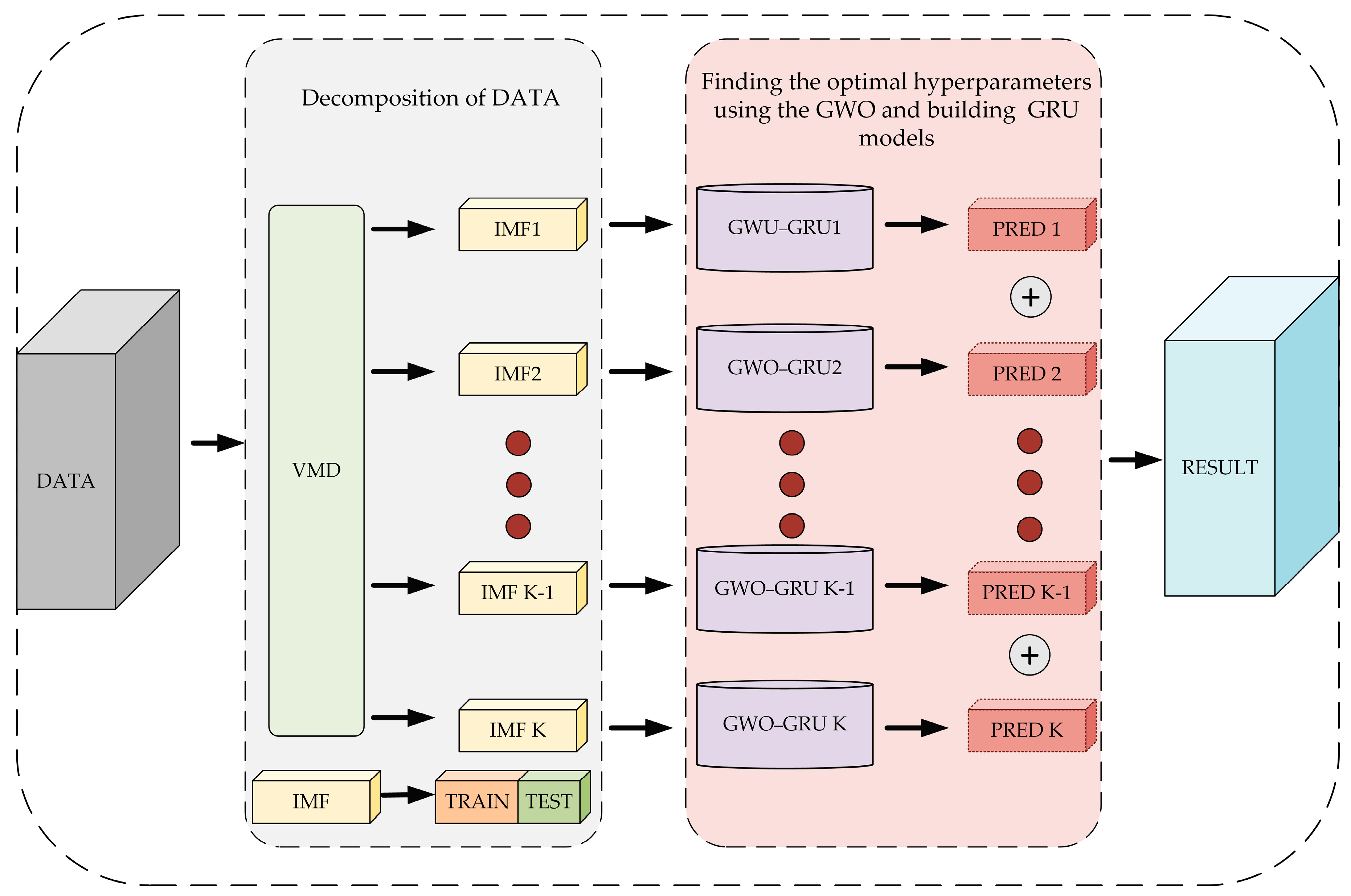
The experiment scheme of this study can be seen in Figure 1. Initially, the raw data were processed in advance to obtain a dataset, which was then divided into K different modal components using the VMD technique, which are represented as intrinsic mode function (IMF)1 to IMF K in Figure 1. Each modal component was divided into a training dataset and a test dataset. The training dataset was used to train the model, and the test dataset was used to evaluate the effectiveness of the model. After that, a GRU neural network was built for each component, and the parameters of each GRU model were adjusted using the GWO algorithm during the training process. These models are represented as GWO–GRU1 to GWO–GRU K in Figure 1. Finally, the prediction results PRED 1 to PRED K of each part were superposed and calculated to obtain the final prediction result.

This paper is structured in a systematic manner to provide a comprehensive overview of the study conducted. The sources of water quality parametric data acquisition are discussed in Section 2, along with the initial processing of the acquired data to ensure a quality dataset. Following this, Section 3 delves into the methodology and theoretical basis used in this study, offering a detailed description of the approach taken. Moving on to Section 4, the experimental procedure and results of the water quality parametric forecasting models are presented, accompanied by a comparison of the outcomes of each model. The effectiveness and reliability of the models were thus thoroughly analyzed and evaluated. Furthermore, Section 5 examines the limitations of the research presented in this paper, while also highlighting potential avenues for future research and development in this field. Lastly, in Section 6, a summary of the entire paper is provided, encapsulating the conclusions drawn from this study.

2. Data Acquisition and Preprocessing

2.1. Data Acquisition

The data for this study were collected from a water quality parameter monitoring system at a water treatment company situated in Changchun, which is in Jilin Province in the northeastern part of China. The study sites and data sources are shown in Figure 2. This system utilizes sensors to sample and detect the water in the water treatment tank and upload the water quality parametric data to a water quality monitoring platform for monitoring and obtaining the water quality parameters, including the pH, DO, COD, among other relevant factors.

Among the common water quality parameters, the dissolved oxygen value is a fundamental indicator of the self-purification capacity of water. The recovery and stability of dissolved oxygen in a water body indicates its self-purification capacity. Concurrently, dissolved oxygen is a fundamental requisite for the survival of aquatic organisms. Consequently, the monitoring and forecasting of the dissolved oxygen value of a water body is of paramount importance for a water treatment plant to formulate water quality treatment measures [42]. In this paper, we employed 900 sets of acquired dissolved oxygen data to construct a forecasting model for water quality parameters. The sampling frequency of the data was one hour, and the data were subjected to analysis and forecasting. Furthermore, the acquired data underwent preprocessing to enhance their suitability for the establishment of forecasting models.

2.2. Data Cleaning

Abnormalities in the acquisition of parameters, delivery of data, and external environmental fluctuations can result in the occurrence of missing data and obvious outliers in the obtained water quality parameter data. Consequently, it is essential that data cleansing is in place prior to model building. In this paper, we identified and removed outliers from the raw data using the box plot technique. When a data value exceeded the maximum value or was lower than the minimum value, it was regarded as an outlier. In the original dataset arranged in ascending order, the lower quartile (Q1) and upper quartile (Q3) correspond to the 25th and 75th percentiles, respectively, while the median is denoted as Q2. Figure 3 and

Table 1. Methods of identifying outliers.

Standard of Judgment	Verdict
x > Q3 + 1.5 (Q3 − Q1) or x < Q1 − 1.5 (Q3 − Q1)	Outlier
x > Q3 + 3 (Q3 − Q1) or x < Q1 − 3 (Q3 − Q1)	Extreme

provide further details on this methodology.

In order to maintain the integrity and validity of the data, we employed the box plot technique to identify and eliminate six obvious outliers in the dissolved oxygen dataset utilized in this investigation, and these outliers were eliminated in order to provide a quality dataset for the subsequent training of the model. The specific elimination process is illustrated in Figure 4, with the red dots representing the screened out obvious outliers.

Once the values were eliminated using the box plot, the empty data points were replaced with interpolated values, following the equation presented as Formula (1):

$$x_k=x_h+\frac{(x_b-x_h)(k-h)}{b-k}$$

(1)

where $x_k$ denotes the missing data to be filled in, $x_h$ denotes the data at the previous sampling point, and $x_b$ denotes the data at the subsequent sampling point. $k$, $h$, and $b$ denote the locations of the sampling points corresponding to the data. The results of 900 sets of DO data after data cleaning are shown in Figure 5.

2.3. Data Normalization

To expedite the rate at which the data gradient declined during the training phase of the water quality parameter forecasting model, it was essential to preprocess the data. This involved normalizing all values to fall within the [0, 1] range. Subsequently, 70% of this normalized dataset served as the training set, while the remaining 30% was designated as the test set. The training set was employed to calibrate the model, optimizing the model parameters within the defined bounds. The test set was then utilized to evaluate the model’s predictive accuracy. Upon completing the predictions, the data were reverted to their original scale. If $X_{\max }$ and $X_{\min }$ represent the highest and lowest values of the dissolved oxygen sequence, respectively, the normalized value for an original value $X$ in the dissolved oxygen sequence is denoted as $x$. The method of normalizing data was carried out using the following equation:

$$x=\left(X-X_{\min }\right)/\left(X_{\max }-X_{\min }\right)$$

(2)

3. Theory and Methods

3.1. Modal Decomposition Methods

3.1.1. Empirical Mode Decomposition (EMD)

EMD, a method for processing signals in the time–frequency domain, is suitable for signals that are both nonlinear and non-stationary. This approach eliminates the need for defining basis functions and instead separates signals based on their time-scale properties. Through the EMD technique, time series data are broken down into multiple intrinsic mode function (IMF) sequences and a single RES sequence sorted by frequency, starting from the highest to the lowest. Each IMF series captures unique characteristics of the original data at varying frequencies, while the RES sequence captures the overall trend. The decomposition process of EMD for a given time series data includes the following steps:

Step 1. Obtain the maximum value and minimum value of the original sequence, use the interpolation function to fit the original sequence, obtain the upper envelope and lower envelope, record the mean values of the upper envelope and the lower envelope as $m(t)$, and convert the original sequence subtracted $m(t)$ from $x(t)$ to get the new sequence $h_1(t)$. The formula for $h_1(t)$ is the following:

$$h_1(t)=x(t)-m(t)$$

(3)

Step 2. The $h_1(t)$ sequence also needs to be verified, so verify that the number of extreme points and zero-crossing points of the entire sequence is equal, and verify whether the average values of the upper envelope and lower envelope are zero. If the above conditions are met, $h_1(t)$ is the first IMF component. If not, the first step needs to be repeated until the conditions are met.

Step 3. Subtract $h_1(t)$ from $x(t)$ to get the new sequence as the original sequence and repeat the above steps until the final IMF sequence is a monotonic sequence. The decomposition result is expressed as the following:

$$x(t)={\displaystyle \sum _1^n{h}_i(t)}+res(t)$$

(4)

where $n$ denotes the number of decompositions, $h_i(t)$ is the $i-th$ IMF component, and $res(t)$ is the residual sequence.

We used the EMD method to decompose the DO data used in this article, obtain eight IMF components and one RES component, and draw their spectrum diagrams to facilitate our comparison with the decomposition results of the VMD method. The EMD decomposition results and the spectrum diagrams corresponding to each component are shown in Figure 6.

3.1.2. Variational Mode Decomposition (VMD)

The nonlinearity and volatility of water quality parametric data are key characteristics. In this study, the VMD method was utilized for decomposing the changes in water quality parametric data. VMD, which stands for variational mode decomposition, is based on solid theoretical principles. Unlike the EMD method, VMD employs a non-recursive strategy to extract signal components. By iteratively adjusting the center frequency and bandwidth, VMD effectively resolves challenges such as error transmission and modal overlap which are commonly encountered in traditional modal decomposition methods. The fundamental mathematical formulations of the VMD method are presented as the following:

$$\underset{\left\{u_k\right\}\left\{{\omega }_k\right\}}{\min }\left\{{\displaystyle \sum _k\Vert {\partial }_t\left[\left(\delta (t)+\frac{j}{\pi t}\right)\ast u_k(t)\right]e^{-j{\omega }_{k}t}\Vert \begin{array}{c}2\\ 2\end{array}}\right\}$$

(5)

$$\mathrm{s}.\mathrm{t}.{\displaystyle \sum _k{u}_k=f}$$

(6)

where $u_k(t)=\left\{u_1,u_2,\cdots u_k\right\}$ is the decomposed K modes, ${\omega }_k$ denotes the central frequency of each modal component, ${\partial }_k$ denotes the partial derivation of moment $\mathrm{t}$, ${\delta }_k$ denotes the impulse function, $j$ represents an imaginary unit, and the sum of the signals of every modal component is denoted as $f$.

Figure 7 presents the results of the component modes obtained from the VMD decomposition of the DO data and the frequency spectra for each component. Key factors in using VMD include determining the penalty parameter α and the number of modes K. Despite the VMD algorithm’s strong performance in signal decomposition, it has several notable limitations. VMD is highly sensitive to parametric choices, making it difficult to determine optimal values for α and K, which directly impacts the quality of the decomposition. Additionally, VMD’s computational demands are high, especially when processing high-frequency complex signals, which can result in extended computation times. It is also susceptible to noise and initial conditions, potentially causing mode mixing or generating spurious components, thereby affecting the decomposition accuracy. This study calculated the central frequencies for each mode after decomposing the original water quality data using VMD. When the central frequencies of the decomposed modes are very close, this suggests that the number of modes has reached the desired level. Using the central frequency method, the number of decomposed modes was determined to be K = 8, with α set to 2500.

Mode mixing means that in EMD, the spectra of different IMFs overlap each other, resulting in the inability of each IMF to be clearly separated, resulting in a poor decomposition effect. This phenomenon can clearly be observed in Figure 6b,d,f in Section 3.1.1, where the spectrum overlap of each IMF component is serious. The VMD method improves the problem of mode mixing by introducing regularization terms and parametric adjustment mechanisms. VMD can separate each IMF more accurately, making the decomposition results more accurate. The examples shown as Figure 7b,d well proved this result. The overlap degree of the spectrum of the eight IMF components obtained by VMD decomposition significantly improved, which was beneficial to the data modeling prediction.

3.2. Neural Network Methods

3.2.1. LSTM Neural Network

An LSTM neural network is derived from enhancing an RNN model. In comparison to the RNN model, LSTM integrates three gating units including an input gate, a forget gate, and an output gate. The input gate is responsible for reading data, while the forget gate filters and transmits data, and the output gate manages backward passes and data outputs. These units address the gradient-vanishing issue encountered in RNN training, leading to a significant enhancement in learning accuracy. Additionally, the memory unit within an LSTM effectively handles the intricate patterns within time series data. Figure 8 illustrates the model structure of the LSTM, where $f_t$ denotes the output value of the forget gate, $X_t$ is the input value at moment $t$, $h_{t-1}$ denotes the state value of the hidden layer at moment $t-1$, $i_t$ denotes the state value of the input gate, $C_t$ denotes the internal memory unit, $O_t$ denotes the output value of the output gate, and $\sigma$ and $\tanh$ denote the activation function and hyperbolic tangent function, respectively.

The forget gate determines whether to retain the memory information of the previous moment and the amount of previous moment information that needs to be retained at the current moment. It determines what information is important and what information can be ignored through weights. The specific formula of the forgetting gate is the following:

$$f_t=\sigma \left(W_f\cdot \left[h_{t-1},X_t\right]+b_f\right)$$

(7)

where $W_f$ is the weight matrix of $f_t$ at moment $t$ and $b_f$ is the bias.

The input gate determines how much new information is added to the memory unit at the current time. The calculation formulas of the input gate and memory unit candidate state ${\tilde{C}}_t$ are the following:

$$i_t=\sigma \left(W_i\cdot \left[h_{t-1},X_t\right]+b_i\right)$$

(8)

$${\tilde{C}}_t=\tanh \left(W_C\cdot \left[h_{t-1},X_t\right]+b_c\right)$$

(9)

where $W_i$ is the weight matrix of $i_t$ at moment $t$, $W_c$ is the weight matrix of ${\tilde{C}}_t$ at moment $t$, and $b_f$ and $b_c$ are the biases. “[]” denotes the connection of two matrices.

The function of the output gate is to filter the contents of the memory unit so that only the part that passes through the output gate will be output to the hidden state. The calculation formula of the output gate is the following:

$$O_t=\sigma \left(W_o\left[h_{t-1},x_t\right]+b_o\right)h_t$$

(10)

where $W_o$ is the weight matrix of $O_t$ at moment $t$ and $b_o$ is the bias.

3.2.2. GRU Neural Network

The internal structure of an LSTM neural network is more complex, and it is difficult to adjust its parameters, which leads to longer time spent on model training. CHO et al. proposed a simplified version of an LSTM called GRU. The cell structure of a GRU neural network is shown in Figure 9.

Figure 9 illustrates that the GRU’s model architecture is comparatively more straightforward than that of the LSTM model. In practice, the GRU model requires less training time than the LSTM model, offering similar predictive accuracy. GRU integrates the input gate and forget gate of LSTM into a single update gate, reducing the memory module to only two gating components: the update gate and the reset gate. The update gate, represented as $Z_t$, manages the degree to which previous data state information is incorporated into the current state. A higher value of the update gate indicates that the present neuron retains more historical information, while the previous neuron retains comparatively less. The primary function of the update gate is to refresh the memory and discern long-term patterns in the water quality data sequence. The formula for the update gate to capture information can be expressed as the following:

$$Z_t=\sigma \left(W_Z\cdot \left[h_{t-1},X_t\right]\right)$$

(11)

The reset gate, denoted as $R_t$, plays a crucial role in assessing the extent of historical information retention. A lower reset gate value signifies a higher retention of past historical data, which is conducive to capturing the short-term patterns in the water quality parametric data. The formula for the reset gate to obtain information is the following:

$$R_t=\sigma \left(W_r\cdot \left[h_{t-1},X_t\right]\right)$$

(12)

where $h_t$ denotes the output state of the unit at moment $t$ and ${\tilde{h}}_t$ denotes the implied state value of $h_t$. This value is utilized for storing the data of the present unit and transmitting it to the subsequent unit, while the estimated value for the previous moment’s output is computed as

$${\tilde{h}}_t=\tanh \left(W_{\tilde{h}}\cdot \left[r_t\ast h_{t-1},X_t\right]\right)$$

(13)

The forecasted outcomes of the water quality parameter data can be expressed as

$$h_t=\left(1-Z_t\right)\ast h_{t-1}+Z_t\ast {\tilde{h}}_t$$

(14)

where $X_t$ denotes the input data value at the current moment $t$, $h_{t-1}$ is the output value of the water quality parameter data in the memory cell at moment $t-1$, $W_z$, $W_r$, and $W_{\tilde{h}}$ denote the weight matrix in the cell, “[]”denotes the connection of two matrices, “$\ast$” denotes the matrix product, $\sigma$ is the activation function, and $\tanh$ is the bisecting curve of the activation function.

3.3. Grey Wolf Optimizer (GWO)

Within the GRU model, specific parameters function as internal variables that are capable of automatic modification and refinement throughout the training phase. On the other hand, external variables, known as model hyperparameters, play a crucial role in achieving distinct goals and must undergo continual adjustments. Manually altering these hyperparameters is clearly not recommended. In this study, a technique is suggested for intelligently modifying the hyperparameters of the GRU model with the application of the grey wolf optimizer. The grey wolf optimizer utilizes the root mean square error (RMSE) as its fitness function and finetunes the hyperparametric values of the model to enhance the prediction accuracy to its optimal level. GWO, an intelligent optimization algorithm introduced by Australian researcher Mirjalili, is founded on grey wolves’ group predatory actions, enabling the attainment of an equilibrium between local optimization and wide-ranging exploration. The algorithm simulates the competitive and cooperative behaviors of grey wolves in their populations, whose strict adherence to a social hierarchy provides inspiration for the algorithm. The structure of the GWO first mimics the social hierarchy of the pack by grading the wolves differently, with the highest-ranked $\alpha$ wolf being the leader of the pack and in charge of decision-making within the pack, followed by the $\beta$ and $\delta$ wolves, which correspond to the three best-adapted parameters, respectively, and the rest of the grey wolves labeled as $\omega$. The society ranks of the grey wolf population are shown in Figure 10.

The iterative process of the algorithm guides the movement of ω wolves through $\alpha$, $\beta$, and $\delta$ wolves to achieve global optimization. The hunting behavior of the grey wolves’ group is shown as the following:

$$\overrightarrow{D}=\left|\overrightarrow{C}\cdot {\overrightarrow{X}}_P(t)-\overrightarrow{X}(t)\right|$$

(15)

$$\overrightarrow{X}(t+1)={\overrightarrow{X}}_P(t)-\overrightarrow{A}\cdot \overrightarrow{D}$$

(16)

where ${\overrightarrow{X}}_P$ denotes the current location vector of the prey, $\overrightarrow{D}$ denotes the location gap between the grey wolf and prey, $\overrightarrow{X}(t)$ denotes the current location vector of the individual grey wolf, $\overrightarrow{X}(t+1)$ denotes the direction of the next movement of the individual grey wolf, and $\overrightarrow{A}$ and $\overrightarrow{C}$ denote the coefficient vectors. The coefficient vectors are shown as the following:

$$\overrightarrow{A}=2\overrightarrow{a}\cdot {\overrightarrow{r}}_1-\overrightarrow{a}$$

(17)

$$\overrightarrow{C}=2{\overrightarrow{r}}_2$$

(18)

$$\overrightarrow{a}(t)=2(1-t/M)$$

(19)

where ${\overrightarrow{r}}_1$ and ${\overrightarrow{r}}_2$ are randomly generated vectors in [0, 1], $\overrightarrow{a}$ is a linear convergence factor whose number decreases linearly from 2 to 0 with constant iterations, and $M$ is the largest number of iterations. Suppose $\alpha$, $\beta$, and $\delta$ are the three optimal solutions obtained during the iterative process of GWO, such that the $\omega$ wolf updates its position based on the positions of the first three wolves. The location update formula is the following:

$$\{\begin{array}{c}{\overrightarrow{D}}_{\alpha }=\left|{\overrightarrow{C}}_1\cdot {\overrightarrow{X}}_{\alpha }-\overrightarrow{X}\right|\\ {\overrightarrow{D}}_{\beta }=\left|{\overrightarrow{C}}_2\cdot {\overrightarrow{X}}_{\beta }-\overrightarrow{X}\right|\\ {\overrightarrow{D}}_{\delta }=\left|{\overrightarrow{C}}_3\cdot {\overrightarrow{X}}_{\delta }-\overrightarrow{X}\right|\end{array}$$

(20)

$$\{\begin{array}{c}{\overrightarrow{X}}_1={\overrightarrow{X}}_{\alpha }-{\overrightarrow{A}}_1\cdot {\overrightarrow{D}}_{\alpha }\\ {\overrightarrow{X}}_2={\overrightarrow{X}}_{\beta }-{\overrightarrow{A}}_2\cdot {\overrightarrow{D}}_{\beta }\\ {\overrightarrow{X}}_3={\overrightarrow{X}}_{\delta }-{\overrightarrow{A}}_3\cdot {\overrightarrow{D}}_{\delta }\end{array}$$

(21)

where ${\overrightarrow{D}}_{\alpha }$, ${\overrightarrow{D}}_{\beta }$, and ${\overrightarrow{D}}_{\delta }$ are the positional gaps between $\alpha$, $\beta$, $\delta$, and other individuals, ${\overrightarrow{X}}_{\alpha }$, ${\overrightarrow{X}}_{\beta }$, and ${\overrightarrow{X}}_{\delta }$ are the positions of $\alpha$, $\beta$, and $\delta$, respectively, and ${\overrightarrow{C}}_{\alpha }$, ${\overrightarrow{C}}_{\beta }$, and ${\overrightarrow{C}}_{\delta }$ are the associated random vectors. ${\overrightarrow{X}}_1$, ${\overrightarrow{X}}_2$, and ${\overrightarrow{X}}_3$ denote the direction and distance of movement toward $\alpha$, $\beta$, and $\delta$, respectively, and ${\overrightarrow{A}}_1$, ${\overrightarrow{A}}_2$, and ${\overrightarrow{A}}_3$ are vectors of coefficients. From the above equation, the latest position of $\omega$ is expressed as

$$\overrightarrow{X}(t+1)=({\overrightarrow{X}}_1+{\overrightarrow{X}}_2+{\overrightarrow{X}}_3)/3$$

(22)

3.4. VMD–GWO–GRU-Based Forecasting Model for Water Quality Parameters

The VMD–GWO–GRU method was implemented to build the model in this paper. Firstly, the preprocessed water quality parametric sequences were decomposed into K modal functions, and then these K modal functions were input into the GRU model, which was enhanced through the GWO algorithm, to individually create predictive models. The resulting predictions were combined linearly to obtain the final forecasted water quality parameters. Figure 11 illustrates the process of determining the optimal hyperparameters for the GRU neural network using the GWO algorithm.

The detailed steps involved in constructing the model are outlined below.

Step 1. Obtain water quality parametric data and perform data preprocessing, including outlier removal and missing value supplementation.

Step 2. Applying the VMD technique for modal decomposition in the denoising of parameters related to water quality, utilize the method of central frequency to establish the decomposition of the sequence of water quality parameters into eight distinct sequences showcasing varying frequency attributes. Consequently, a total of eight modal components can be derived.

Step 3. Set the population size and determine the iteration count for GWO. Set the initial values of the GRU network parameters and the range of hyperparametric values, with the hyperparameters of each model carried out by the GWO to find the optimal parameters, and use the values corresponding to the optimal fitness values as the hyperparameters of the model for model training.

Step 4. Divide the training set and test set of each component, and build a GWO–GRU model separately for training and prediction. The prediction results for each component can be obtained, and the model’s evaluation metrics can be calculated.

Step 5. Superimpose the prediction results of each component to obtain the final prediction result, and calculate the evaluation index of the final prediction result.

In this paper, we chose a group of fundamental parameters that were substantiated by various research for their forecasting impacts, such as the quantity of input layers, the quantity of output layers, the quantity of completely connected layers, the decreasing factor for the learning rate, the regularization factor, the algorithm for gradient descent, and the function for activation, and the specific parameters are detailed in

Table 2. Basic parameters of the GRU model.

Parameter	Value
Input layer	15
Output layer	1
Fully connected layer	1
Regularization factor	0.001
Learning rate drop factor	0.2
Gradient descent algorithm	Adam
Activation function	ReLU

.

Meanwhile, the GRU neural network presents numerous hyperparameters open to optimization. The GWO algorithm was employed to pinpoint key parameters affecting model accuracy, including the hidden layer unit count, initial learning rate, and iteration quantity. The GWO algorithm’s population size was fixed at 5, with 20 iterations set for optimization. Refer to

Table 3. Optimization intervals for model hyperparameters.

Parameter	Value
Number of hidden layer units	[50, 200]
Iterations	[200, 500]
Initial learning rate	[0.001, 0.02]

for details on the optimization intervals for the aforementioned hyperparameters.

3.5. Principles of Evaluation of the Model

To assess the performance of the prediction model for water quality parameters in this paper, and to quantitatively analyze the deviation between the predicted values and the actual values of the obtained water quality parameters, the model evaluation indexes utilized in this paper included the RMSE and MAPE, and the formulas for the mentioned evaluation indicators are presented as the following:

$$RMSE=\sqrt{\frac{1}{n}{\displaystyle \sum _{i=1}^n{({\tilde{y}}_i-y_i)}^2}}$$

(23)

$$MAPE=\frac{1}{n}{\displaystyle \sum _{i=1}^n\frac{\left|{\tilde{y}}_i-y_i\right|}{y_i}}\times 100\%$$

(24)

where $n$ denotes the number of sample points at which the data were collected, $y_i$ denotes the original actual value of the DO data, and ${\tilde{y}}_i$ denotes the predicted value of the DO data.

4. Comparisons and Results

4.1. Simulation Comparison of LSTM Model and GRU Model

To verify that the GRU model selected in this study trained faster than the LSTM model, as well as to confirm that both the GRU and LSTM models yielded similar prediction results for water quality parameters, we constructed individual LSTM and GRU models for comparison. We utilized 900 preprocessed DO datasets for training and testing purposes. The basic parameters for both models were kept constant, as depicted in Table 2, where the number of iterations was set to 400, the hidden layer units were configured to 100, and the initial learning rate was established at 0.001.

Figure 12 displays the test set prediction outcomes of the two individual models. The original data are represented by the black curve, while the prediction results and absolute error curves of the LSTM model are shown in red, and the prediction results and absolute error curves of the GRU model are in blue. As can be seen from Figure 12, under the same parameters, the independent GRU model was closer to the real value than the independent LSTM model for the DO data, the lag of the prediction results was weaker, the absolute error between the predicted value and the real value was smaller, and the fitting prediction effect on water quality parameters was better.

According to

Table 4. Evaluation indicators for LSTM and GRU.

Model	RMSE	MAPE	Training Duration
LSTM	0.49517	4.3764%	65.23 s
GRU	0.40713	3.4169%	36.35 s

, the GRU model exhibited a modeling speed 44.3% faster than the LSTM model, while GRU showed a significant advantage over LSTM in training speed, primarily due to its simpler structure with only two gate mechanisms: a reset gate and update gate. In contrast, LSTM includes an input gate, forget gate, and output gate, along with additional cell state updates. GRU has fewer parameters because its gate mechanisms share some parameters and only update their hidden state, whereas each gate mechanism in LSTM has independent weight matrices. Furthermore, the GRU model demonstrated a decreased RMSE and MAPE of 17.8% and 21.9%, respectively, compared to the LSTM model, indicating its suitability for predicting water quality parametric data. It is worth noting that when building a single GRU model, we manually input the hyperparameters of the GRU model based on experience. This was obviously uneconomical and may have had an impact on the final prediction results of the GRU model. Introducing intelligent optimization algorithms for hyperparametric or parametric optimization can improve this shortcoming.

4.2. Simulation Comparison of GRU, GWO–GRU, and GWO–LSTM Models

This study presents a new approach for optimizing the hyperparameters of the GRU model and the LSTM model using a grey wolf optimizer. A dataset comprising 900 preprocessed DO datasets was utilized to train the GRU, GWO–GRU, and GWO–LSTM models separately. The prediction results are visualized in Figure 13, with the original data curve shown in black, the prediction results and absolute errors of the GRU model in blue, the prediction results and absolute errors of the GWO–GRU model in purple, and the prediction results and absolute errors of the GWO–LSTM model in green.

By employing GWO to finetune the GRU and LSTM model parameters, including the number of hidden layer units, the initial learning rate, and the number of iterations, the best parameter set [101, 0.005426, 392] was identified after 20 iterations. Specifically, the optimal number of hidden layer units was 101, the most effective initial learning rate was 0.005426, and the ideal number of iterations was 392. The best parameter set [98, 0.008426, 389] for LSTM was identified after 20 iterations. Implementing these parameters in the GRU model and the LSTM model led to a substantial enhancement in model performance. The evaluation indicators presented in

Table 5. Evaluation indicators for the GRU, GWO–GRU, and GWO–LSTM models.

Model	RMSE	MAPE
GRU	0.40713	3.4169%
GWO–LSTM	0.41804	3.8265%
GWO–GRU	0.34507	2.8886%

compared the performance of the GRU model with that of the GWO–GRU model and the GWO–LSTM model. The GWO–GRU model demonstrated superior results, with a 22.2% decrease in RMSE and a 22.3% decrease in MAPE compared to the standalone GRU model. The RMSE and MAPE of the GWO–LSTM model in Table 5 decreased by 16.5% and 12.6%, respectively, compared with the LSTM model in Table 4. These findings underscore the efficacy of leveraging the GWO algorithm for parameter optimization in enhancing the predictive accuracy of the GRU model and the LSTM model. In the course of this experiment, it was found that when using the GWO to adaptively adjust the hyperparameters of the GRU model, the modeling time of the GWO–GRU model increased significantly. The reason for this shortcoming is that when using the grey wolf optimization algorithm to iterate, in order to improve the prediction performance of the model and obtain more accurate prediction results, the number of iterations will affect the modeling speed of the model.

4.3. Simulation Comparison of GWO–GRU Model and VMD–GWO–GRU Model

To enhance the predictive performance of the water quality parametric model, this study employed the VMD method to decompose the DO dataset. This decomposition allowed for a more accurate representation of the variations in DO characteristics. After fully decomposing the DO dataset using the VMD method, eight components were obtained, and then GRU models were established for the eight obtained components. Each GRU model used the GWO algorithm to find the optimal hyperparameters to establish eight GWO–GRU models. The prediction results obtained by each component were superimposed to obtain the final prediction result. The population size and number of iterations of GWO remained the same as above and were also set to 5 and 20. The hyperparametric combinations of each GWO–GRU model after optimization by the GWO algorithm are shown in

Table 6. Hyperparameters for each component model.

Component	Number of Hidden Layer Units	Initial Learning Rate	Iterations
VMD-IMF 1	121	0.01645	313
VMD-IMF 2	94	0.00723	365
VMD-IMF 3	104	0.00649	378
VMD-IMF 4	91	0.00775	432
VMD-IMF 5	113	0.00622	500
VMD-IMF 6	50	0.00576	474
VMD-IMF 7	85	0.00365	447
VMD-IMF 8	102	0.01032	442

.

The combined prediction results, as shown in Figure 14, highlight a significant improvement in the predictive accuracy of the water quality parameter model. The original data are represented by the black curve, while the purple curve shows the predictions and absolute errors of the GWO–GRU model, and the orange curve displays the predictions and absolute errors of the VMD–GWO–GRU model. As can be seen in Figure 14a, the VMD–GWO–GRU model we proposed significantly improved the lag of the prediction results. The prediction results were closer to the real monitoring data. It was better at predicting some mutation values, but it was found that unfortunately, the predictive effect was not good at the 100th to 125th sampling points. This may have been caused by the VMD method’s insufficient decomposition of the original data. However, the method we proposed has obvious advantages in overall prediction accuracy. It can be seen that the absolute error of the predicted value of the VMD–GWO–GRU model relative to the true value is smaller in Figure 14b.

Table 7. Evaluation indicators for the GWO–GRU and VMD–GWO–GRU models.

Model	RMSE	MAPE
GWO–GRU	0.34507	2.8886%
VMD–GWO–GRU	0.20227	1.8811%

displays the RMSE and MAPE outcomes for both the VMD–GWO–GRU model and the GWO–GRU model. In contrast to the GWO–GRU model, the VMD–GWO–GRU model demonstrated a reduction of 23.9% and 25.9% in its RMSE and MAPE, correspondingly. The experimental results show that the VMD method can be used to decompose original data into multiple components and effectively extract the change characteristics of a water quality parametric sequence. This helps the GWO–GRU model to fully learn the change characteristics of each component. The data in Table 7 support the effectiveness of the VMD method we introduced in the data processing stage, and more accurate prediction results for future data values of water quality parameters were obtained.

5. Discussion

The VMD–GWO–GRU model adopted in this paper integrates the GWO algorithm, VMD algorithm, and GRU neural network, which fully exploit the feature information hidden in the dissolved oxygen data and enhance the precision of water quality parametric prediction, but there are some aspects that need to be further discussed and improved.

In this paper, we employed the VMD decomposition technique to further break down dissolved oxygen data, thereby fully capturing the water quality parameters’ trends. The findings indicate that the VMD approach offers significant advantages in data decomposition, addressing the modal aliasing issue present in conventional signal decomposition algorithms, and enhancing the prediction accuracy of dissolved oxygen data. Additionally, we utilized the central frequency method to determine the number of decompositions, specifically eight. Future research can explore the use of intelligent optimization algorithms (such as PSO and GWO) to automatically adjust key parameters of the VMD algorithm, such as α and K, overcoming the difficulties of manual parameter tuning. By selecting appropriate objective functions as the basis for optimization, signal loss due to insufficient decomposition can be avoided, thereby enhancing the robustness and efficiency of VMD in practical applications.

Some hyperparameters of the GRU neural network were obtained by the grey wolf optimizer, and the experimental results showed that the GRU model established by applying the combination of these hyperparameters achieved a good predictive effect on the dissolved oxygen data. The number of experiments could be increased in future research to find better hyperparametric optimization intervals, reduce the number of iterations of GWO, and increase the speed of modeling. Meanwhile, the VMD–GWO–GRU model proposed in this paper currently focuses on predicting only one parameter, the DO level, with both model inputs and outputs being DO. Future research could explore the modeling prediction of more water quality parameters (including ammonia nitrogen level and pH) to improve the overall generalizability of the model. In addition, future studies should focus more on exploring the linkages between these water quality parameters, using more parameters as auxiliary variables for predicting a particular water quality parameter to improve the performance of the prediction model, and investigating the effectiveness of the model proposed in this paper in different regions and water body environments to provide a more reliable tool for water quality monitoring and treatment.

6. Conclusions

In this study, a VMD–GWO–GRU model for predicting water quality parameters was developed based on the historical correlation and fluctuation characteristics of these parameters. The main conclusions drawn are the following:

(1)

Box plots and linear interpolation were utilized to remove and supplement anomalous data, the raw water quality parametric data were decomposed using the VMD decomposition algorithm, and the main changed characteristics of the water quality parameter series were extracted.

(2)

Aiming at the problem that the traditional GRU model needs to manually adjust its model parameters, good results were achieved by using the grey wolf optimizer for adaptive optimization of the model parameters, modeling and predicting the dissolved oxygen data after VMD decomposition, respectively, and inputting the optimal hyperparameters into the model.

(3)

The VMD–GWO–GRU water quality parametric prediction model developed in this paper achieved better results in both the RMSE and MAPE evaluation indexes, indicating that the model has lower error and a higher prediction accuracy in water quality parametric prediction compared to the unoptimized model. Moreover, the lag of the water quality parametric prediction model was significantly improved.

The model VMD–GWO–GRU proposed in this study can offer superior predictive performance for anticipating water quality parameters. It is capable of forecasting the trajectory of these parameters, offering dependable guidance for water treatment companies to enhance their capacity and efficiency.

References

1. Han, D.; Currell, M.J.; Cao, G. Deep challenges for China’s war on water pollution. Environ. Pollut. 2016, 218, 1222–1233. [Google Scholar] [CrossRef] [PubMed]
2. Lowe, M.; Qin, R.; Mao, X. A review on machine learning, artificial intelligence, and smart technology in water treatment and monitoring. Water 2022, 14, 1384. [Google Scholar] [CrossRef]
3. Zulkifli, C.Z.; Garfan, S.; Talal, M.; Alamoodi, A.; Alamleh, A.; Ahmaro, I.Y.; Sulaiman, S.; Ibrahim, A.B.; Zaidan, B.; Ismail, A.R.J.W. IoT-based water monitoring systems: A systematic review. Water 2022, 14, 3621. [Google Scholar] [CrossRef]
4. Namugize, J.; Jewitt, G. Sensitivity analysis for water quality monitoring frequency in the application of a water quality index for the uMngeni River and its tributaries, KwaZulu-Natal, South Africa. Water SA 2018, 44, 516–527. [Google Scholar] [CrossRef]
5. Neale, P.A.; Escher, B.I.; de Baat, M.L.; Dechesne, M.; Deere, D.A.; Enault, J.; Kools, S.A.; Loret, J.-F.; Smeets, P.W.; Leusch, F.D. Effect-based monitoring to integrate the mixture hazards of chemicals into water safety plans. J. Water Health 2022, 20, 1721–1732. [Google Scholar] [PubMed]
6. Volf, G.; Sušanj Čule, I.; Žic, E.; Zorko, S. Water Quality Index Prediction for Improvement of Treatment Processes on Drinking Water Treatment Plant. Sustainability 2022, 14, 11481. [Google Scholar] [CrossRef]
7. Li, T.; Lu, J.; Wu, J.; Zhang, Z.; Chen, L. Predicting aquaculture water quality using machine learning approaches. Water 2022, 14, 2836. [Google Scholar] [CrossRef]
8. Schellart, A.; Tait, S.; Ashley, R. Towards quantification of uncertainty in predicting water quality failures in integrated catchment model studies. Water Res. 2010, 44, 3893–3904. [Google Scholar] [CrossRef] [PubMed]
9. Fan, F.; Qiao, Z.; Wu, L. Using a grey multivariate model to predict impacts on the water quality of the Zhanghe River in China. Water Sci. Technol. 2021, 84, 777–792. [Google Scholar] [CrossRef]
10. Huang, H.; Wang, Z.; Xia, F.; Shang, X.; Liu, Y.; Zhang, M.; Dahlgren, R.A.; Mei, K. Water quality trend and change-point analyses using integration of locally weighted polynomial regression and segmented regression. Environ. Sci. Pollut. Res. 2017, 24, 15827–15837. [Google Scholar] [CrossRef]
11. Ilić, M.; Srdjević, Z.; Srdjević, B. Water quality prediction based on Naïve Bayes algorithm. Water Sci. Technol. 2022, 85, 1027–1039. [Google Scholar] [CrossRef] [PubMed]
12. Hmoud Al-Adhaileh, M.; Waselallah Alsaade, F. Modelling and prediction of water quality by using artificial intelligence. Sustainability 2021, 13, 4259. [Google Scholar] [CrossRef]
13. Wu, J.; Zhang, J.; Tan, W.; Lan, H.; Zhang, S.; Xiao, K.; Wang, L.; Lin, H.; Sun, G.; Guo, P. Application of time serial model in water quality predicting. Comput. Mater. Contin. 2023, 74, 67–82. [Google Scholar] [CrossRef]
14. Sarkar, M.R.; Anavatti, S.G.; Dam, T.; Ferdaus, M.M.; Tahtali, M.; Ramasamy, S.; Pratama, M. GATE: A guided approach for time series ensemble forecasting. Expert Syst. Appl. 2024, 235, 121177. [Google Scholar] [CrossRef]
15. Wu, H.; Xu, J.; Wang, J.; Long, M. Autoformer: Decomposition transformers with auto-correlation for long-term series forecasting. Adv. Neural Inf. Process. Syst. 2021, 34, 22419–22430. [Google Scholar]
16. Sarkar, M.R.; Anavatti, S.G.; Dam, T.; Pratama, M.; Al Kindhi, B. Enhancing wind power forecast precision via multi-head attention transformer: An investigation on single-step and multi-step forecasting. In Proceedings of the 2023 International Joint Conference on Neural Networks (IJCNN), Gold Coast, Australia, 18–23 June 2023; pp. 1–8. [Google Scholar]
17. Ahn, J.M.; Kim, J.; Kim, H.; Kim, K. Harmful Cyanobacterial Blooms forecasting based on improved CNN-Transformer and Temporal Fusion Transformer. Environ. Technol. Innov. 2023, 32, 103314. [Google Scholar] [CrossRef]
18. Ehteram, M.; Ahmed, A.N.; Sherif, M.; El-Shafie, A. An advanced deep learning model for predicting water quality index. Ecol. Indic. 2024, 160, 111806. [Google Scholar] [CrossRef]
19. Tan, W.; Zhang, J.; Wu, J.; Lan, H.; Liu, X.; Xiao, K.; Wang, L.; Lin, H.; Sun, G.; Guo, P. Application of CNN and long short-term memory network in water quality predicting. Intell. Autom. Soft Comput. 2022, 34, 1943–1958. [Google Scholar] [CrossRef]
20. Pang, J.; Luo, W.; Yao, Z.; Chen, J.; Dong, C.; Lin, K. Water quality prediction in urban waterways based on wavelet packet Denoising and LSTM. Water Resour. Manag. 2024, 38, 2399–2420. [Google Scholar] [CrossRef]
21. Jiange, J.; Liqin, Z.; Senjun, H.; Qianqian, M. Water quality prediction based on IGRA-ISSA-LSTM model. Water Air Soil Pollut. 2023, 234, 172. [Google Scholar] [CrossRef]
22. Liu, X.; Shi, Q.; Liu, Z.; Yuan, J. Using LSTM neural network based on improved PSO and attention mechanism for predicting the effluent COD in a wastewater treatment plant. IEEE Access 2021, 9, 146082–146096. [Google Scholar] [CrossRef]
23. Yan, Y.; Zhang, W.; Liu, Y.; Li, Z. Simulated annealing algorithm optimized GRU neural network for urban rainfall-inundation prediction. J. Hydroinform. 2023, 25, 1358–1379. [Google Scholar] [CrossRef]
24. Chi, D.; Huang, Q.; Liu, L. Dissolved oxygen concentration prediction model based on WT-MIC-GRU—A case study in Dish-Shaped lakes of poyang Lake. Entropy 2022, 24, 457. [Google Scholar] [CrossRef]
25. Xu, J.; Wang, K.; Lin, C.; Xiao, L.; Huang, X.; Zhang, Y. FM-GRU: A time series prediction method for water quality based on seq2seq framework. Water 2021, 13, 1031. [Google Scholar] [CrossRef]
26. Lin, C.; Weng, K.; Lin, Y.; Zhang, T.; He, Q.; Su, Y. Time series prediction of dam deformation using a hybrid STL–CNN–GRU model based on sparrow search algorithm optimization. Appl. Sci. 2022, 12, 11951. [Google Scholar] [CrossRef]
27. Yang, H.; Liu, S. Water quality prediction in sea cucumber farming based on a GRU neural network optimized by an improved whale optimization algorithm. PeerJ Comput. Sci. 2022, 8, e1000. [Google Scholar] [CrossRef]
28. Tikhamarine, Y.; Souag-Gamane, D.; Ahmed, A.N.; Kisi, O.; El-Shafie, A. Improving artificial intelligence models accuracy for monthly streamflow forecasting using grey Wolf optimization (GWO) algorithm. J. Hydrol. 2020, 582, 124435. [Google Scholar] [CrossRef]
29. Bao, X.; Jiang, Y.; Zhang, L.; Liu, B.; Chen, L.; Zhang, W.; Xie, L.; Liu, X.; Qu, F.; Wu, R. Accurate Prediction of Dissolved Oxygen in Perch Aquaculture Water by DE-GWO-SVR Hybrid Optimization Model. Appl. Sci. 2024, 14, 856. [Google Scholar] [CrossRef]
30. Wang, Z.; Qiu, J.; Li, F. Hybrid models combining EMD/EEMD and ARIMA for long-term streamflow forecasting. Water 2018, 10, 853. [Google Scholar] [CrossRef]
31. Jiao, J.; Ma, Q.; Huang, S.; Liu, F.; Wan, Z. A hybrid water quality prediction model based on variational mode decomposition and bidirectional gated recursive unit. Water Sci. Technol. 2024, 89, 2273–2289. [Google Scholar] [CrossRef]
32. Boudraa, A.-O.; Cexus, J.-C. EMD-based signal filtering. IEEE Trans. Instrum. Meas. 2007, 56, 2196–2202. [Google Scholar] [CrossRef]
33. Zare, A.; Ozdemir, A.; Iwen, M.A.; Aviyente, S. Extension of PCA to higher order data structures: An introduction to tensors, tensor decompositions, and tensor PCA. Proc. IEEE 2018, 106, 1341–1358. [Google Scholar] [CrossRef]
34. Zhang, Y.; Li, C.; Jiang, Y.; Sun, L.; Zhao, R.; Yan, K.; Wang, W. Accurate prediction of water quality in urban drainage network with integrated EMD-LSTM model. J. Clean. Prod. 2022, 354, 131724. [Google Scholar] [CrossRef]
35. Wang, W.; Chau, K.; Qiu, L.; Chen, Y. Improving forecasting accuracy of medium and long-term runoff using artificial neural network based on EEMD decomposition. Environ. Res. 2015, 139, 46–54. [Google Scholar] [CrossRef] [PubMed]
36. El Khadiri, K.; Elouaham, S.; Nassiri, B.; El Melhaoui, O.; Said, S.; El Kamoun, N.; Zougagh, H. A Comparison of the Denoising Performance Using Capon Time-Frequency and Empirical Wavelet Transform Applied on Biomedical Signal. Int. J. Eng. Appl. 2023, 11, 358. [Google Scholar] [CrossRef]
37. Rezaiy, R.; Shabri, A. Enhancing drought prediction precision with EEMD-ARIMA modeling based on standardized precipitation index. Water Sci. Technol. 2024, 89, 745–770. [Google Scholar] [CrossRef]
38. Roushangar, K.; Davoudi, S.; Shahnazi, S. Temporal prediction of dissolved oxygen based on CEEMDAN and multi-strategy LSTM hybrid model. Environ. Earth Sci. 2024, 83, 158. [Google Scholar] [CrossRef]
39. Seo, Y.; Kwon, S.; Choi, Y. Short-term water demand forecasting model combining variational mode decomposition and extreme learning machine. Hydrology 2018, 5, 54. [Google Scholar] [CrossRef]
40. Hu, Y.; Dai, B.; Yang, Y.; Zhao, D.; Ren, H. Sample Generation Method Based on Variational Modal Decomposition and Generative Adversarial Network (VMD–GAN) for Chemical Oxygen Demand (COD) Detection Using Ultraviolet Visible Spectroscopy. Appl. Spectrosc. 2023, 77, 1173–1180. [Google Scholar] [CrossRef]
41. He, M.; Wu, S.; Huang, B.; Kang, C.; Gui, F. Prediction of total nitrogen and phosphorus in surface water by deep learning methods based on multi-scale feature extraction. Water 2022, 14, 1643. [Google Scholar] [CrossRef]
42. Feng, D.; Han, Q.; Xu, L.; Sohel, F.; Hassan, S.G.; Liu, S. An ensembled method for predicting dissolved oxygen level in aquaculture environment. Ecol. Inform. 2024, 80, 102501. [Google Scholar] [CrossRef]
Figure 1. Research plan chart.
Applsci 14 06111 g001
Figure 2. (a) Changchun’s geographical location and (b) on-site acquisition equipment.
Applsci 14 06111 g002
Figure 3. Structure of box plot.
Applsci 14 06111 g003
Figure 4. Box plot of DO data.
Applsci 14 06111 g004
Figure 5. Preprocessed dissolved oxygen data.
Applsci 14 06111 g005
Figure 6. EMD decomposition results for DO data: (a) IMF1–IMF4 sequences, (b) IMF1–IMF4 spectrum diagrams, (c) IMF5–IMF8 sequences, (d) IMF5–IMF8 spectrum diagrams, (e) IMF9 sequence, and (f) IMF9 spectrum diagram.
Applsci 14 06111 g006aApplsci 14 06111 g006b
Figure 7. VMD decomposition results for DO data: (a) IMF1–IMF4 sequences, (b) IMF1–IMF4 spectrum diagrams, (c) IMF5–IMF8 sequences, and (d) IMF5–IMF8 spectrum diagrams.
Applsci 14 06111 g007
Figure 8. Schematic structure of the LSTM neural network.
Applsci 14 06111 g008
Figure 9. Structure of the GRU model.
Applsci 14 06111 g009
Figure 10. Society ranks of the grey wolf population.
Applsci 14 06111 g010
Figure 11. Flowchart of optimization of the VMD–GWO–GRU model.
Applsci 14 06111 g011
Figure 12. (a) LSTM and GRU prediction results, and (b) LSTM and GRU absolute errors.
Applsci 14 06111 g012
Figure 13. (a) GRU and GWO–GRU and GWO–LSTM prediction results, and (b) GRU and GWO–GRU and GWO–LSTM prediction absolute errors.
Applsci 14 06111 g013
Figure 14. (a) GWO–GRU and VMD–GWO–GRU prediction results, and (b) GWO–GRU and VMD–GWO–GRU prediction absolute errors.
Applsci 14 06111 g014