Evaluating the Accuracy of the Reverse Engineering Process of Worn, Non-Standard Spur Gears—Pilot Studies

Abstract

For years, gears have been self-made by many industrial plants as substitutes (custom spare parts) for original parts from the manufacturer. This common practice uses a process called reverse engineering (RE). However, in the available scientific database, it is difficult to find articles about the accuracy of such a process. And while it is obvious that in order to obtain the most accurate quality of such a process, modern measurement techniques (coordinate, optical) should be used, most companies cannot afford to purchase such equipment. Reproducing gear geometry is difficult. But the issue of RE of non-standard gears seems to be even more difficult. This is why the authors undertook pilot studies to assess the accuracy of the RE process of worn, non-standard spur gears using conventional techniques and measuring instruments. Eight gears were tested, the module of which ranges from 1.020 to 4.98 mm. The key parameter was selected to estimate the accuracy of the process—the base pitch. The goal is to determine the value of the profile angle. Eleven models were proposed to estimate the nominal tolerance field, using various types of random data distribution. The tested gears were made in IT grade: 6, 7, 8, and 9 according to DIN 3961. Vernier disk micrometers were used for research. It has been shown that the nominal module does not have to be treated as a random variable in the population. Equation of identity was developed, allowing conversion of any gear with specific values of geometric parameters into an identical gear with alternative values of these parameters. The most effective estimating model was selected taking into account the symmetric Student–Fisher distribution with a confidence level of 60%. However, it is not possible to correctly reproduce the geometry of the gear wheel in that way. The following aspects should be taken into account: type and degree of mode of failure, number of load cycles, rotational speed, direction of rotation, material, type of thermochemical treatment, and torque. A simulation using FEM should be performed to determine the fatigue plastic deformations and diagnose their impact on the geometric dimensions of the gear wheel.

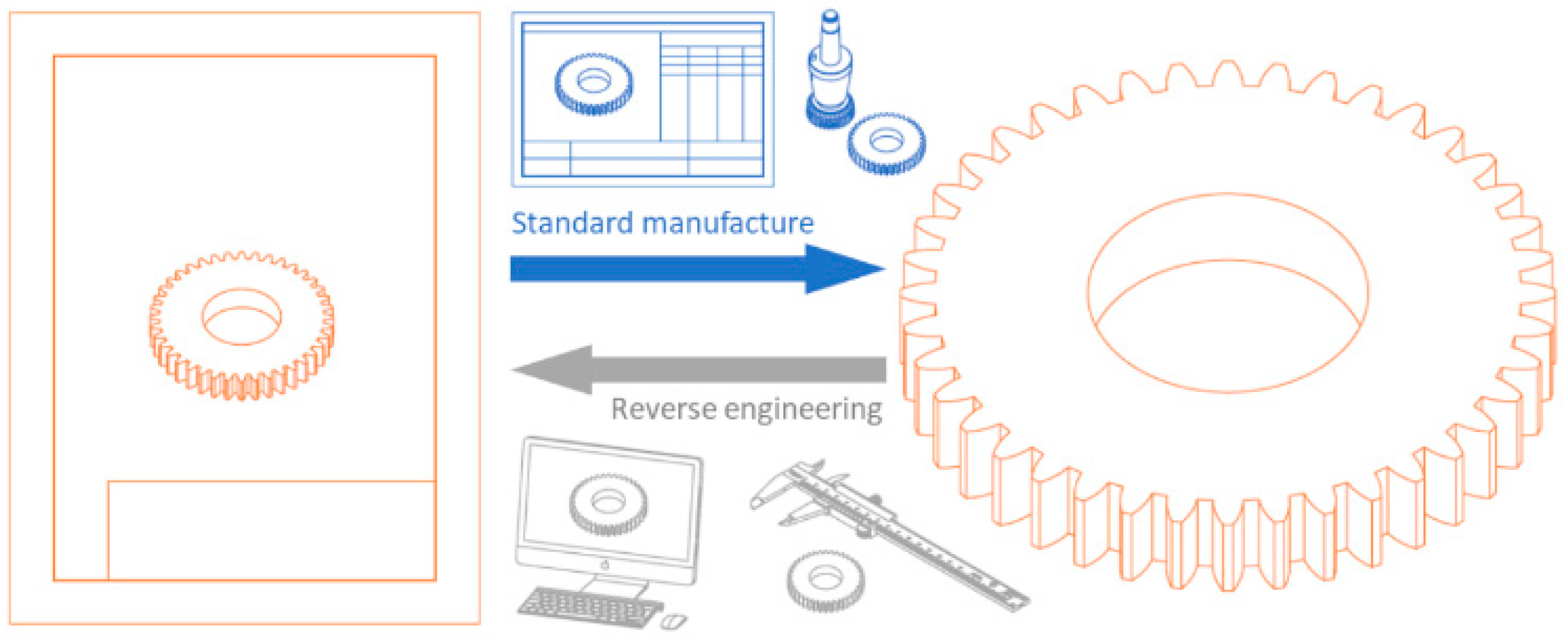
1. Introduction

Although RE is used in many branches of modern industry, in gear engineering, it particularly concerns the preparation of a technical drawing of a physically existing gear to be measured. On the basis of the technical documentation prepared in this way, it is possible to reproduce this part as a spare part (Figure 1).

The need to make a spare part for the gear wheel on your own may be caused by the lack of availability of the original spare part in the manufacturer’s service box.

Although this practice is known and widely used all over the world, there are no publications in the available scientific databases and literature that indicate the possibility of unambiguously reproducing the geometry of a spur gear with straight teeth using only conventional techniques and measuring instruments. Modern measuring machines (e.g., a specialized four-axis coordinate measuring machine for measuring gears) have built-in modules for reverse engineering. Based on the measurement of the left and right side profiles of the tooth, it is possible to generate the basic geometric parameters of the tested gear. Conventional instruments and techniques are those that do not require the use of modern optical and coordinate measuring machines. This group includes the following: disk micrometer for span measuring (across n teeth), modular caliper for measuring tooth thickness, standard caliper for measuring the addendum diameter and the dedendum diameter, and various types of simple conversion techniques for individual geometric relationships in a gear wheel. In such a process, the aim is to reduce the cost and time associated with measurements. In this work; however, the authors went a step further and touched on the topic of RE for non-standard spur gears. The key issue for this topic is tolerance assignment in RE. Krogstie et al. [1] pay particular attention to the great importance of tolerance engineering for increasing efficiency in designing and manufacturing mechanical parts.

Figure 1. Illustration of the idea of RE for a spur gear [2].

Figure 1. Illustration of the idea of RE for a spur gear [2].

M.A. Sáenz-Nuño et al. [3] presented a useful approach to setting tolerances that are practical for the industry for any mechanical part within RE. The measurements of the parts were made by sufficiently qualified students. Each geometric parameter of the parts tested was measured N times, where the number N varies depending on the part being measured, one of the three: for PR 06 $N\in 〈16 ;32〉$, for PR 08 $N\in 〈5 ;12〉$, and for PR 05 $N\in 〈4 ;7〉$. This is an important suggestion in the context of selecting the type of data dispersion in a statistical study. The four key parameters for developing the results in the cited work were: (i) Average, (ii) Median, (iii) Disper, and (iv) Range. In Section 3.2, IT specification of the cited work, the authors conclude that it is more effective to use the median as the nominal dimension rather than the average. In their analysis, the authors assigned a symmetrical tolerance JS/js according to ISO 286 [4] to each measurement. In the case of gear wheels, there is a specific analogy because the deviations of the geometric parameters of gear wheels are also symmetrical. However, they themselves state in their publication that the scope of the proposed strategy is to be a simple and quick IT estimation procedure, which is why complex estimations of the normal distribution of measurements were not addressed. The classical principle is also preserved in the work cited: $MPE\le 10\%·IT$. In the case of this work, this may not necessarily be maintained due to the much higher precision of gears used in the aviation industry compared to the relatively large error limits of disk micrometers.

The works of George J. Kaisarlis et al. [5,6,7] describe an extensive approach to the allocation of tolerances for test parts (hole and shaft) within RE. They presented a method based on five steps: Step (a) consists of determining the direction of analysis of measurements of diameter, geometric deviations, and surface roughness and determining the measurement uncertainty in relation to the ISO 286 (Fundamental Deviation) standard and/or the ISO 2768 (General Tolerances) standard [8]; Step (b) consists of designating the Sets of candidate IT grades; Step (c) consists of designating the Sets of suggested fits; Step (d), in which the set of suggested fits is limited to obtain the Sets of preferred fits; and Step (e) of selecting the best tolerance match relative to production costs. This work contains many mathematical dependencies that determine the zero-one type of behavior (meeting one condition determines a further action, meeting an alternative condition determines a different action). However, you must pay attention to the following facts: (i) gears are tolerated according to other specialized standards regarding the specific method of dimensioning and tolerating the macro- and microgeometry of gears; (ii) gears cannot be referred to as a male or female member of the assembly against which fits are determined; (iii) the issue of the possibility of using statistical techniques to determine the dispersion of measurement data should also be raised; and (iv) the cited work includes measurements using CMM. Therefore, there is a need to formulate an adequate tolerance allocation model for gears, using conventional techniques and measuring instruments.

Another publication by the same authors, George J. Kaisarlis et al. [9] talks about the use of a knowledge-based system (KBS) for tolerance allocation in RE and also in relation to the use of CMM in measurements. However, the cited work contains a specific algorithm for assigning tolerances for the tested parts within RE (Figure 3 on page 531), which is the inspiration for the authors of this work to create a tolerance allocation model for gears within RE. An aspect contained in the cited work, which the authors considered potentially troublesome in the study of gears, is the use of increments of 0.5 and 0.1 (left side of the algorithm, Figure 3 on page 531 in the cited work) with respect to the NS. Even minor manipulations of the base pitch value of the order of thousandths of a millimeter significantly affect the accuracy of recreating the geometry of the tested wheel. Moreover, conventional measuring instruments have much larger error limits than CMMs.

In [10] by Zhaohui Geng et al., scientists rightly point out that since all parts were received from the original supplier or dismantled from the machines, they have certainly passed quality control by the manufacturer. Therefore, the areas defined by the upper and lower limits of the dimensional values tested should be at least within the original tolerance specifications. However, these types of estimates are conservative because the estimated tolerance areas may be too narrow, which could unnecessarily require high-precision RE manufacturing processes. Four standardized boundary estimators were used to examine a part with nine symmetrically tolerated dimensions and five geometric tolerances: (i) ASME Estimator, (ii) ISO Range Estimator, (iii) ISO 6σ Estimator and (iv) ISO PCR Estimator. As in one of the previously cited works, here the measurements were made using a CMM, by which the researchers indicate that the measurement error of a coordinate measuring machine can be approximated by the DGPPR (datum-guided partial Procrustes registration) method proposed by Geng and Bidanda [11], which is much smaller than the variability between parts. Therefore, measurement errors can be ignored in the study of the tolerance estimation of original manufacturing processes. The presentation of the estimated tolerance fields in the RE process is provided in Tables 1 and 2 of the cited work. Table 2 calculates the ratios of the estimated tolerance fields to the original tolerance fields included in the manufacturing drawing of the tested part. Values are given as percentages. The estimator ratio is not determined (“–” in the table) if both extreme values of the estimated tolerance field are not within the range of the original tolerance field. For example, in the ISO PCR Estimator (Ratio) for Size 1 in Table 2 of the cited work, there is an error. The value should be 0.5%, not 0.05%. Evidence: for Size 3 $={0.550}^{″}\pm {0.001}^{″}$ (according to Figure 9), the original tolerance zone is equal $T_{true}={0.002}^{″}$. The ISO Range Estimator shows an estimated tolerance zone of $T_{desig}={0.55000}^{″}-{0.54999}^{″}={0.00001}^{″}$ (according to

Table 1. Basic geometric parameters of the gears tested.

No.	Mark	z	m	α	y	x	c*
1	16	13	3.020	21.018°	0.9924	−0.0421	0.1675
2	13	18	4.980	26.325°	0.7950	+0.0695	0.3830
3	2	42	4.029	21.104°	1.0189	+0.4184	0.1463
4	2	42	4.029	21.104°	1.0189	+0.4184	0.1463
5	3	30	4.410	25.572°	0.9012	−0.5423	0.5196
6	5	29	1.020	22.888°	0.9283	−0.5263	0.3002
7	11	17	4.980	19.358°	1.0065	−0.0641	0.1958
8	6	18	4.980	26.325°	0.8632	+0.0695	0.2525

). And so:

$$ISO Range Estimator \left(Ratio\right)=\frac{{0.00001}^{″}}{{0.00200}^{″}}·100\%=0.5\%$$

(1)

However, both the value of 0.05% and the corrected value of 0.5% indicate a very narrow overlap (interference) of the tolerance fields, which would require increasing the machining accuracy of the re-manufactured part by several classes. In the work cited, the scientists assumed that the data distribution was normal and symmetric, and the average value was approximately equal to the unknown nominal value, which is why they used the coefficient $C_p$ instead of the coefficient $C_{pk}$. They also adopted a standard coefficient value of 1.33. In the cited work, the scientists presented a wide range of discussions and conclusions related to the estimators of the ASME [12] and ISO [13] standards. The authors will apply the same selected estimators here to verify the applicability to non-standard gears.

The aim of this work is to initially check whether it is possible to correctly recreate the geometry of a worn, non-standard spur gear using conventional techniques and measuring instruments commonly available in most design offices and laboratory workshops. The most effective model should be selected among the available statistical models that allow the estimation of the tolerance zone. The available scientific database does not contain appropriate models determining the accuracy of the reverse engineering process of gears. None of them discusses the issue of correctly reproducing the IT grade of the tested gear and, therefore, the permissible errors.

2. Materials and Methods

2.1. Tested Gear Wheels

The study examined worn, non-standard spur gears obtained from the aviation industry under an agreement. Due to legal restrictions, it is not possible to show the original technical drawing. The photos of the wheels were also cropped so that it was not possible to graphically associate the tested wheels with any commercial product (Figure 2).

The word non-standard here refers to different aspects: normal, high, or low teeth; a relatively small profile shift factor; an unusual value of the profile angle; a custom module value; the value of the radial clearance coefficient exceeding the commonly accepted range (Table 1). The wheels are worn to varying degrees, but none of them have noticeable chipped teeth (without scoring or pitting).

2.2. Conventional Measuring Instruments Used

A regular electronic caliper was used for the preliminary measurements to identify the modulus value. For further measurements, Vernier disk micrometers with various measurement ranges were used, depending on the size of the gear wheel: 25–50 mm, 50–75 mm, and 75–100 mm. All of the above-mentioned devices belong to the category of conventional, commonly used measuring devices. It is about reducing costs and time in the reverse engineering process, as well as the practicality of this process in the everyday design approach.

2.3. Conventional Measurement Techniques Used

Regarding the initial measurements with a standard caliper to determine the modulus value, the following measurements were taken:

• measurement of the tip diameter and measurement of the root diameter in the case of gears with an even number of teeth,
• measurement of the distance AB from the tip of the tooth to the bottom of the opposite root in the cases of gears with an odd number of teeth.

These are classic methods of recreating the geometry used in the case of cylindrical gears. In the second case, the following formula was necessary:

$$\overline{AB}=\left(\frac{d}{2}+h_a\right)+\left(\frac{d}{2}-h_f\right)$$

(2)

In the case of determining the base pitch using a disk micrometer, span measurements were made across n and n + 1 teeth, previously determining the optimal number of teeth using the following formula:

$$n=\frac{1}{\pi }\left[\sqrt{{\left(\frac{z+2x}{\cos \alpha }\right)}^2-z^2}-z\mathrm{inv}\alpha -2x\tan \alpha \right]+0.5$$

(3)

It was also checked whether, for gears with a relatively small number of teeth and a large module, it is possible to measure across n + 1 teeth by checking the maximum number of teeth for span measurement using the following formula:

$$n_{max}=\frac{1}{\pi }\left[\frac{\sqrt{d_a^2-d_b^2}}{m\cos \alpha }-z\mathrm{inv}\alpha -2x\tan \alpha \right]+0.5$$

(4)

In future research, this will be related to the need to use a workshop microscope, which will change the MPE of the device and, consequently, the final measurement uncertainty.

The measurement methodology and the metrological steps taken as part of it coincide with those presented by K. Konecki et al. in [14].

Measurements were made of 10 randomly selected teeth of each gear in a random cross-sectional plane across the width of the gear. Total $8\times 10\times 2=160$ measurements.

2.4. The Model Used Compares the Nominal Gear with the Recreated Gear

In order to estimate the accuracy of reverse engineering, a key geometric parameter of the gear wheel, which is the base pitch, was selected to determine the correctness of the geometry reconstruction. This position of the involute, which unwinds from the base circle on which the tested base pitch is measured, is crucial for the quality of reproducing the geometry of the gear wheel. The original values of this parameter were compared with their recreated values. Recreating the value of the shift factor, which plays an equally important role in the context of tooth thickness, is left for a future article.

2.5. The Model Used for the Statistical Analysis of the Results

The following models were used in the work to estimate the tolerance field of the basic pitch:

Model 0 is implicitly the nominal dimension and its deviations (the original tolerance zone).

Model I assumes a normal, symmetric distribution. The ISO estimator will be here $\pm 3\sigma$, also called estimator $6\sigma$. Average is used as NS:

$$p_{b_{design}}=\overline{X}=\frac{1}{N}·\sum _{i=1}^N{X}_i$$

(5)

Model II assumes a symmetrical normal distribution. The ISO estimator here will be PCR. Average is used as NS. The estimated tolerance zone is calculated according to the following formula:

$$T_{desig}=6·\sigma ·C_p$$

(6)

where the $C_p$ coefficient is equal to 1.33.

Model III is the Disper parameter calculated according to the following formula:

$$Disper=2·\max \left[\left(Max-Average\right),\left(Average-Min\right)\right]$$

(7)

The half Disper is the upper and lower deviations of the base pitch. Average is used as NS.

Model IV and Model V are the Range parameters calculated according to the formula:

$$R=Max-Min$$

(8)

Half-Range is the upper and lower deviation of the base pitch. As NS, Median:

$$p_{b_{design}}=Med=\frac{X_{i_{max}}+X_{i_{min}}}{2}$$

(9)

and Average are used for the models.

From Model VI to Model XI, it is the adoption of a symmetric S-F distribution. The ISO estimator will be $\pm t_{N, \alpha }{\sigma }_r$. The confidence level was assumed appropriately for the models: $\alpha =99\%$, $\alpha =95\%$, $\alpha =90\%$, $\alpha =80\%$, $\alpha =60\%$ and $\alpha =40\%$. Average is used as NS.

The standard deviation was calculated in various ways. When a symmetric Gaussian distribution was adopted, the standard deviation for the sample was calculated according to the following formula:

$$\sigma =\sqrt{\frac{1}{N}·\sum _{i=1}^N{\left(X_i-\overline{X}\right)}^2}$$

(10)

When a symmetric S-F distribution was adopted, the standard deviation of the sample was calculated according to the formulas:

$${\sigma }_{t-S}={\sigma }_r·t_{N,\alpha }$$

(11)

$$S=\sqrt{\frac{1}{N-1}·\sum _{i=1}^N{\left(X_i-\overline{X}\right)}^2}$$

(12)

$${\sigma }_r=\frac{S}{\sqrt{N}}$$

(13)

The value of Student’s t-coefficient depends on the adopted confidence level.

The data necessary to present the results were calculated according to the following formulas:

$$T_{true}=USL-LSL$$

(14)

$$Estimator \left(Ratio\right)=\frac{T_{desig}}{T_{true}}·100\%$$

(15)

The measurement uncertainty of the disk micrometer should be added to each estimated zone; however, in order to determine the value of the base pitch, measurements were made twice: first across n + 1 teeth and then across n teeth. Each of these measurements is burdened with the MPE of the micrometer. The uncertainty of a micrometer measurement is the geometric sum of such components [15] as:

• micrometer screw and nut error $F=\pm 3 \mathsf{\mu }\mathrm{m}$,
• flatness error of the anvil and spindle $T_p=\pm 0.9 \mathsf{\mu }\mathrm{m}$,
• parallelism error of the anvil and spindle measuring surfaces $T_r=2 \mathsf{\mu }\mathrm{m}$,
• perpendicularity error of the spindle measuring surfaces relative to its axis $T_v=1 \mathsf{\mu }\mathrm{m}$,
• error in the lower measurement range $f_A=2 \mathsf{\mu }\mathrm{m}$,
• bow deformation error for $P=10 N\approx 2 \mathsf{\mu }\mathrm{m}$,
• error related to the elastic deformation of the measured object $\approx 1 \mathsf{\mu }\mathrm{m}$,
• error related to immobilizing the spindle with a clamp $\approx 2 \mathsf{\mu }\mathrm{m}$,
• roughness error of the measurement surfaces $\le 0.08 \mathsf{\mu }\mathrm{m}$,
• parallax error $\approx 1 \mathsf{\mu }\mathrm{m}$,
• temperature error (for steel and $\Delta T=\pm 5 °\mathrm{C}$ negligible),
• micrometer setting error $\approx 1 \mathsf{\mu }\mathrm{m}$.

In this study, it was assumed that the limit error for a single measurement with a disk micrometer was equal to $\delta =\pm 4 \mathsf{\mu }\mathrm{m}$ for the measurement range $25÷50 \mathrm{m}\mathrm{m}$, $\delta =\pm 4 \mathsf{\mu }\mathrm{m}$ for the measurement range $50÷75 \mathrm{m}\mathrm{m}$, and $\delta =\pm 5 \mathsf{\mu }\mathrm{m}$ for the measuring range $75÷100 \mathrm{m}\mathrm{m}$, for the device used during the tests according to DIN 863 and DIN 863-1 [16], factory marked 40 SM [17,18].

All guidelines for the course of calculations, based on the above-mentioned principles, were taken from the monograph by Jezierski J. [19], which is a classic bibliographic position for Polish scientists, metrologists, and designers.

3. Additional Observation

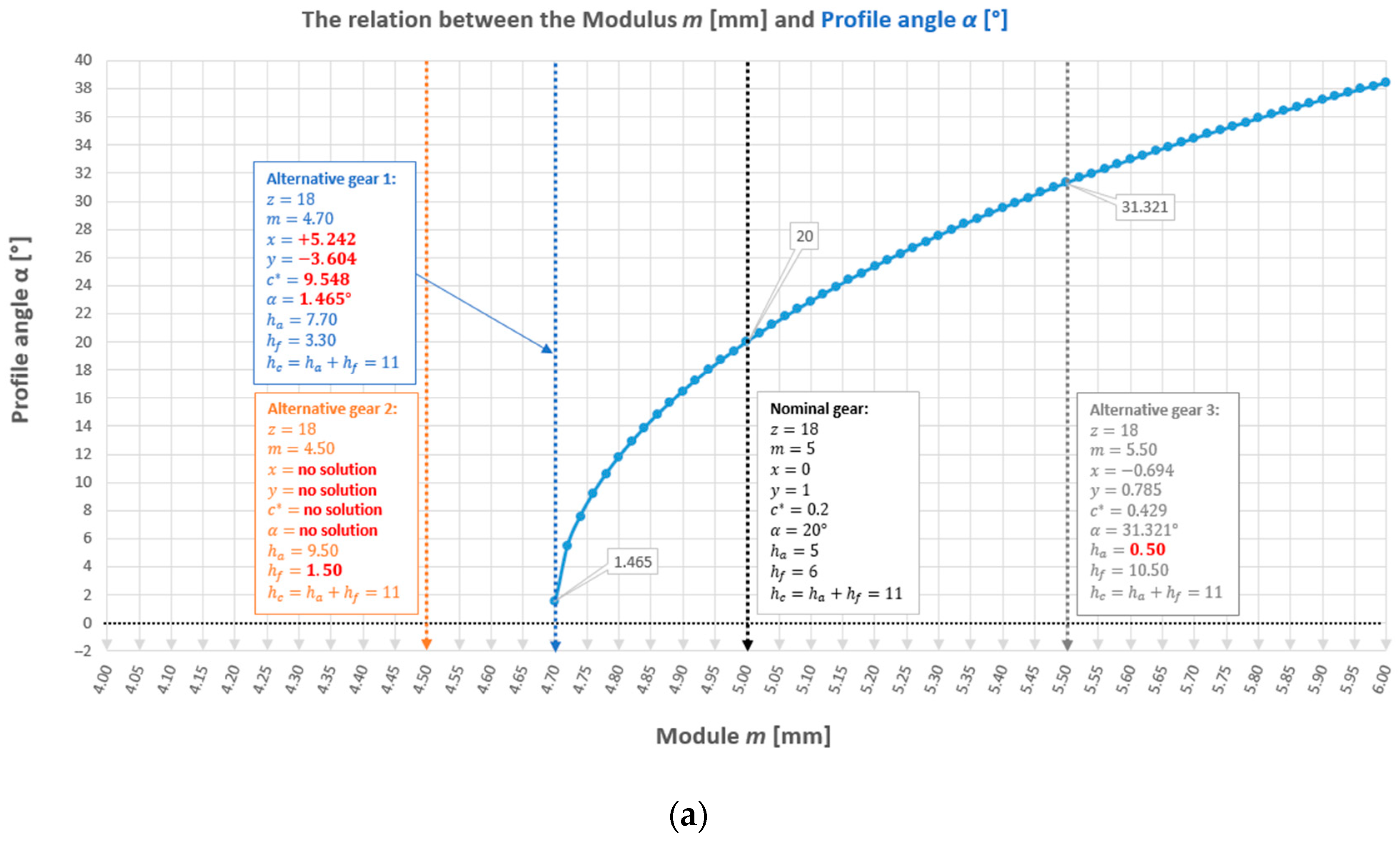
Module as a Random Variable in the Population

During the research, a puzzling fact for the authors was whether the reproduced value of the module should be treated as a random variable. Is it not the case that the tested modules are a sample from the population that can reproduce the values of the nominal modules? The authors tried to answer the question of the relationship between the original gear wheel with a non-standard module and the reconstructed gear wheel with a different, but still non-standard, module, both very similar in value. It is important that we are talking about nominal geometries here without taking into account real and observed dimensions. We are only talking about the tolerable dimensions according to ISO and the generally tolerable dimensions included in the technical drawing of the original gear wheel and the recreated gear wheel. The authors wanted to answer whether it is necessary at all (and if so, to what extent) to get as close as possible to the original value of the nominal gear module when reconstructing the geometry of this gear.

It was found that for two wheels to be the same, they must have identical tooth thickness at any diameter. The base diameter of both wheels must be the same. Taking the above into account, after several transformations, an equation with two unknowns was finally obtained, allowing the selection of a pair of parameters, module-shift factor, which can be used as an alternative to the originally assumed/calculated ones. The diameter of the base is treated here as a known value.

First, the formula $s=\left(\frac{\pi }{2}+2·x·\tan \alpha \right)·m$ was inserted into the expression $s_x=d_x·\left(\frac{s}{d}+\mathrm{i}\mathrm{n}\mathrm{v}\alpha -\mathrm{i}\mathrm{n}\mathrm{v}{\alpha }_x\right)$:

$$s_x=d_x·\left[\frac{\left(\frac{\pi }{2}+2·x·\tan \alpha \right)·m}{z·m}+\mathrm{i}\mathrm{n}\mathrm{v} \alpha -\mathrm{i}\mathrm{n}\mathrm{v} {\alpha }_x\right]$$

(16)

Then, two steps were performed: The following were inserted into the above: $\mathrm{i}\mathrm{n}\mathrm{v}\alpha =\tan \alpha -\overline{\alpha }$ and $\mathrm{i}\mathrm{n}\mathrm{v}{\alpha }_x=\tan {\alpha }_x-{\overline{\alpha }}_x$ and then $\alpha ={\cos }^{-1}\left(\frac{d_b}{z·m}\right)$ and ${\alpha }_x={\cos }^{-1}\left(\frac{d_b}{d_x}\right)$:

$$s_x=d_x·\left\{\frac{\frac{\pi }{2}+2·x·\tan \left[{\cos }^{-1}\left(\frac{d_b}{z·m}\right)\right]}{z}+\left\{\tan \left[{\cos }^{-1}\left(\frac{d_b}{z·m}\right)\right]-{\cos }^{-1}\left(\frac{d_b}{z·m}\right)\right\}-\left\{\tan \left[{\cos }^{-1}\left(\frac{d_b}{d_x}\right)\right]-{\cos }^{-1}\left(\frac{d_b}{d_x}\right)\right\}\right\}$$

(17)

After transformation and simplification, the following equation was obtained, called the Equation of Identical Gears (EIG) [20,21]:

$$x=z·\frac{\frac{s_x}{d_x}-\frac{\pi }{2·z}-\left\{\tan \left[{\cos }^{-1}\left(\frac{d_b}{z·m}\right)\right]-{\cos }^{-1}\left(\frac{d_b}{z·m}\right)\right\}+\left\{\tan \left[{\cos }^{-1}\left(\frac{d_b}{d_x}\right)\right]-{\cos }^{-1}\left(\frac{d_b}{d_x}\right)\right\}}{2·\tan \left[{\cos }^{-1}\left(\frac{d_b}{z·m}\right)\right]}$$

(18)

This proves that you should not worry about the fact that the recreated value of the module may most likely be completely different than the original value, because, in the context of the correctness of the geometry reconstruction process, it has no mathematical significance. Therefore, the module cannot be used as a parameter to compare the original wheel with the recreated wheel. An explanation of this aspect is presented in

Table 2. Alternative sets of geometric parameters of the same gear (example data).

m	α	y	x	c*	pb [mm]	dx [mm]	sx [mm]
1.98	18.344°	1.028	−0.0876	0.200	5.904	113	1.485
1.97	17.445°	1.034	+0.0507	0.165
1.96	16.490°	1.032	+0.1981	0.180
1.95	15.466°	1.020	+0.3576	0.216

, which shows that the use of alternative parameters does not change either the base pitch or the tooth thickness measured along the arc of any chosen circle.

An interesting issue worth paying attention to in future research is the fact that, depending on the set (Table 2), the same gear is shifted negatively ($x<0$), and sometimes positively ($x>0$). Therefore, if there was a need for a direct tabular comparison of the basic geometric parameters of the original wheel (which would constitute the first row of the table) with the parameters of the recreated wheel (which would constitute the third row of the table), one more middle row of the table should be added with the values of the parameters of the recreated wheel converted thanks to EIG, bringing this wheel to a common module with the original wheel.

Table 3. Comparison of the recreated wheel with the original wheel (example data).

	m	α	y	x	c*
The recreated gear	1.97	17.538°	1.0339	+0.0509	0.1658
The identical gear (EIG)	1.98	18.432°	1.0278	−0.0874	0.1666
The nominal gear	1.98	18.344°	1.0280	−0.0876	0.2

explains this.

The situation is different from a technological perspective if the wheel being recreated is to be manufactured using hobbing processing. Previously, two Greek scientists, Christos Spitas and Vasilios Spitas [22,23], showed that, in such a case, the filet changes slightly, thus causing a change in the thickness of the tooth at the base. This, in turn, directly affects the bending strength of the tooth.

However, the question must be answered: to what extent can the module be changed in relation to the nominal tested gear so that the reconstructed geometry makes mathematical sense and has practical usefulness in terms of the values of alternative geometric parameters? Such a study will be necessary due to geometric and technological limitations in converting a given set of geometric parameters into an alternative set. Figure 3 shows two graphs for an example of a spur gear with straight teeth and parameters: $z=18$, $m=5$, $x=0$, $y=1$, $c^{*}=0.2$, $\alpha =20°$.

It is clearly visible from Figure 3a that, for module 4.70 (i.e., $\Delta m=0.30 \mathrm{m}\mathrm{m}$), a wheel geometry is achieved, which is impossible from the design point of view (for example, due to the negative whole depth factor $y=-3.604$). This variant is close to the left asymptote of the graph, for which $\alpha =0°$. However, on the right side, where the graph has no limits on the argument domain, theoretically, the value of the module can be increased indefinitely. However, this graph is not coupled with the limit value of the shift factor at which tooth undercutting occurs at the base. The graph presented in Figure 3b is an alternative version of the graph in Figure 3a, with the parameter on the vertical axis changed from the profile angle to the profile shift factor. The same conclusions can be drawn from it, but it additionally shows the shape of the function of the presented relationship. In the future, it is planned to create three-dimensional design maps to enable more effective recognition of the relationships between all three parameters: $m$, $x$, and $\alpha$.

With reference to the previous conclusion, each set of geometric parameters of the gear wheel has its alternative version in an infinite number, but nevertheless within a range limited by the value of the limit shift factor and of the limit whole depth factor. This requires further research in the future. However, during reverse engineering, the authors do not expect to obtain a recreated modulus value that differs significantly from the nominal value.

The confirmation of this non-obvious mathematical phenomenon related to involute profiles is the fact that by examining the gear on a specialized four-axis coordinate measuring machine (Wenzel WGT 600) using the TReverse module, it is possible to obtain alternative values of geometric parameters, depending on the selected area on the tooth side, which was measured with a measuring probe during the measurement. An example of two alternative sets is shown in Figure 4.

The equation discussed here (EIG) can be adapted to gear tests using the finite element method in the strength simulation of gear drives [24]. Due to this, it will be possible to study the impact of a minor manipulation of the modulus value on the strength properties of the gear tooth (this is directly related to the change in the shape of the filet at the base of the tooth).

4. Results and Discussion

4.1. True Deviations and the IT Grade of the Tested Gear Wheel

Figure 5 shows a diagram for selecting the gear accuracy class of the produced gear depending on the industry and the application area. It is expected that each of the wheels tested is made in grades 5 to 10.

The tested gears could have been manufactured several decades ago. It is therefore impossible to reconstruct the information according to which standard the wheel designer originally calculated the values of permissible deviations. When it comes to the availability of manufacturing deviations in the drawings of the tested wheels, the situation is different. Some drawings clearly show the selected class and the standard, while others lack such information, instead providing the deviations of the selected parameters. To have an increased level of confidence in the authentic accuracy class of the tested wheel, an intermediate solution was chosen, and the values of permissible deviations for class 5 were calculated according to the standard [26]. For the remaining classes, conversion factors consistent with the standard were used. The values of the permissible deviations expressed in [mm] have been rounded to the third decimal place.

Table 4. A list of formulas [25] to calculate the permissible error deviations of individual tooth elements, according to DIN 3961-1953 for IT grade 5 [26]. Values in [μm].

Type of Error	φ	Module Range m [mm]
		do 0.6	od 0.6 do 1.6	od 1.6 do 4	od 4 do 10
Δe Δtp Δo Δt0	1.4/1.6	$$3+0.3m+0.2\sqrt{d}$$ (19)
Δrs	1.4/1.6	$$2.5+0.25m+0.15\sqrt{d}$$ (20)
∑Δt0	1.4/1.6	$$10+m+0.8\sqrt{d}$$ (21)
Δg	1.4	$$1.4+1.85\sqrt{m}+2.06\sqrt[4]{d}$$ (22)	$$1.4+1.85\sqrt{m}+2.18\sqrt[4]{d}$$ (23)	$$1.4+1.85\sqrt{m}+2.30\sqrt[4]{d}$$ (24)	$$1.4+1.85\sqrt{m}+2.43\sqrt[4]{d}$$ (25)
Δr	1.4	$$2+2.57\sqrt{m}+2.89\sqrt[4]{d}$$ (26)	$$2+2.57\sqrt{m}+3.07\sqrt[4]{d}$$ (27)	$$2+2.57\sqrt{m}+3.25\sqrt[4]{d}$$ (28)	$$2+2.57\sqrt{m}+3.45\sqrt[4]{d}$$ (29)
ΔM	1.4	$$1.32+1.7\sqrt{m}+1.95\sqrt[4]{d}$$ (30)	$$1.32+1.7\sqrt{m}+2.06\sqrt[4]{d}$$ (31)	$$1.32+1.7\sqrt{m}+2.18\sqrt[4]{d}$$ (32)	$$1.32+1.7\sqrt{m}+2.3\sqrt[4]{d}$$ (33)

shows the formulas for calculating the permissible error values according to DIN 3961-1953 and the conversion factors.

Table 5. Conversion factors for the deviations of various toothing and engagement errors, according to DIN (TGL), depending on the IT grade. Only grades 5 to 10 are shown.

Type of Error	IT Grade
	5	6	7	8	9	10
Δe Δtp Δo Δt0 Δrz ∑Δt0	1	1.4	1.96	2.74	3.84	6.15
Δg Δr ΔM	1	1.4	1.96	2.74	3.84	5.36

shows the exact values of the conversion factors for the deviations of various errors according to DIN (TGL).

4.2. Measurement Results in Statistical Analysis

The manufacturing drawings contain various types of information, both with respect to geometric deviations and, for example, the conditions for accepting the wheel from quality control. The authors verified the IT grade of the tested gears, bringing all the information on allowed errors to the DIN 3961 standard.

Table 6. Qualification of the tested gears to the appropriate IT grade according to DIN 3961.

Gear		Drawing Information			Calculated Errors in 5 to 10 IT Grades according to DIN 3961						Qualified for IT Grade
No.	Mark	IT Grade Information	According to the Standard	Permissible Errors [mm]	5	6	7	8	9	10
1	16	7	DIN 3967	ΔM = 0.028 Δg = 0.030 Δtp = ?	0.010 0.010 0.005	0.014 0.014 0.007	0.020 0.020 0.010	0.027 0.028 0.014	0.038 0.040 0.020	0.054 0.055 0.032	8
2	13	–	–	ΔM = 0.022 Δg = 0.025 Δtp = ?	0.012 0.013 0.006	0.017 0.018 0.009	0.024 0.025 0.013	0.033 0.036 0.018	0.047 0.050 0.025	0.065 0.070 0.039	7
3	2	–	–	ΔM = 0.035 Δg = 0.037 Δtp = ?	0.013 0.013 0.007	0.018 0.019 0.010	0.025 0.026 0.013	0.034 0.037 0.019	0.048 0.051 0.026	0.067 0.072 0.042	8
4	2	–	–
5	3	–	–	Δtp = 0.010	0.007	0.009	0.013	0.018	0.025	0.040	6
6	5	7	DIN 3962	Δg = 0.030 Δtp = ?	0.008 0.004	0.012 0.006	0.016 0.009	0.023 0.012	0.032 0.017	0.045 0.027	9
7	11	9	DIN	ΔM = 0.024 Δtp = ?	0.012 0.006	0.017 0.009	0.024 0.012	0.033 0.017	0.046 0.024	0.065 0.039	7
8	6	I	industry standard	ΔM = 0.054 Δg = 0.060 Δtp = ?	0.012 0.013 0.006	0.017 0.018 0.009	0.024 0.025 0.013	0.033 0.036 0.018	0.047 0.050 0.025	0.089 0.070 0.039	9

presents the drawing information with analysis in relation to the mentioned standard and the qualification of the wheel to the appropriate IT grade. It was needed, among other things, to determine the deviation of the base pitch, the value of which is reproduced as part of the research presented in this work.

In the case of Gear No. 1 Mark 16, a calculator [27] was used to check the correctness of the drawing and, indeed, for the seventh grade $\Delta g=0.03 \mathrm{m}\mathrm{m}$. Gear No. 4 Mark 2 is the same wheel as Gear No. 3 Mark 2; however, it has significant signs of use, including large oil stains. In the drawing of Gear No. 5 Mark 3, the deviation of the base pitch is given directly. In the drawing of Gear No. 7 Mark 11, the standard number is not provided, but the DIN letter is. In the case of Gear No. 8 Mark 6, the measurement value deviation of 0.054 mm is close to the value of 0.047 mm, which corresponds to grade 9. The deviation of tooth thickness of 0.06 mm is as close to the value of 0.050 mm (grade 9) as to the value of 0.070 mm (grade 10). In both cases, the difference is 0.01 mm. However, due to the fact that the deviation of the measured value at the level of 0.054 mm on the right side is close to the normalized value of 0.047 for grade 9 and is far from the value of 0.089 mm for grade 10, the tested wheel should be classified as grade 9 according to DIN 3961. Figure 6, Figure 7, Figure 8, Figure 9, Figure 10, Figure 11, Figure 12 and Figure 13 show blocks of double graphs created on the basis of measurement data and statistical calculations.

4.3. Synthesis of Results

To begin, all wheels should be compared in the context of the recreated manufacturing IT grade according to DIN 3961 (

Table 7. Recreated IT grades according to DIN 3961 for the tested gears.

Gear Designation	IT Grade
	5	6	7	8	9	10
No. 1 Mark 16				x
No. 2 Mark 13			x
No. 3 Mark 2				x
No. 4 Mark 2				x
No. 5 Mark 3		x
No. 6 Mark 5					x
No. 7 Mark 11			x
No. 8 Mark 6					x

).

So, there is one gear in grade 6, two gears in grade 7, three gears in grade 8, and two gears in grade 9.

The direction and degree of shift of the graphs relative to the nominal zone were determined. The degree of shift was determined relative to the Average and Median (two parameters that were used as the center of the measurement data distribution). The results are presented in

Table 8. Direction and degree of shift of the graphs of the estimated tolerance zones.

Gear Designation	Direction	Degree of Shift Δ1 and Δ2 [‰]
		Relative to Average	Relative to Median
No. 1 Mark 16	→	1.028	1.254
No. 2 Mark 13	→	0.918	0.704
No. 3 Mark 2	←	0.595	0.722
No. 4 Mark 2	←	5.676	4.109
No. 5 Mark 3	←	0.261	0.181
No. 6 Mark 5	→	0.464	0.972
No. 7 Mark 11	→	1.141	1.141
No. 8 Mark 6	→	0.171	0.009

. Each parameter that better approximates the nominal dimension is marked in green. The following formulas were used:

$${\delta }_1=\frac{\left|NS-Average\right|}{NS}·1000 ‰$$

(34)

$${\delta }_2=\frac{\left|NS-Median\right|}{NS}·1000 ‰$$

(35)

In the case of Gear No. 7 Mark 11, the Average and Median had the same value. Overall, the Average was three times more effective, while the Median was four times more effective. Due to similar results and a relatively small number of tested wheels, it is not possible to select a better parameter that estimates the nominal value of the basic pitch. The shift to the right occurred five times. The shift to the left occurred three times. In subsequent tests, the nature and potential source of wear of the tested gears should be determined. Except in the case of Gear No. 4 Mark 2 (which, by the way, is the same wheel as Gear No. 3 Mark 2, only worn to a different extent and covered with oil stains) and, coincidentally, Gear No. 8 Mark 6 (which performed relatively well compared to the other wheels), all other cases for Average range from 0.261 to 1.141. In the future, we should try to generate average values of the so-called “straightening coefficients”. The idea is to reduce the shifted graph to a nominal field. This will be conducted analytically (by multiplying the center of the distribution by appropriate coefficients) or graphically (by using asymmetric distributions).

The authors assessed the degree of filling of the estimated tolerance field inside the nominal field, i.e., the estimator ratio expressed in [%]. A point allocation matrix was proposed (

Table 9. Estimator Ratio evaluation matrix, expressed in [%].

	IT Grade wg DIN 3961
Model ↓	8	7	8	8	6	9	7	9	Suma pkt.	Occurrence in All Measured Gears?	Verdict
XI	➂			➁	➁				75	YES	Second best
X	➁			➀	➀		➂		110	YES	Best
IX	➀	➂					➁		75	–	–
VIII		➁	➂				➀		70	–	–
VII		➀	➁						60	–	–
VI			➀			➂			45	–	–
V						➁			25	–	–
IV						➁		➂	30	–	–
III						➀		➁	50	–	–
II									0	–	–
I								➀	30	–	–
Gear No.→	1	2	3	4	5	6	7	8
Mark→	16	13	2	2	3	5	11	6
Explanations:					Estimator Ratio > 100%
	➀→	30 points		➀	Estimator Ratio < 100%, 1st place
	➁→	20 points		➁	Estimator Ratio < 100%, 2nd place
	➂→	10 points		➂	Estimator Ratio < 100%, 3rd place
		5 points			Estimator Ratio < 100%

).

However, the above matrix does not directly explain important issues such as how a specific estimator relates to a given IT grade, how narrow the designed tolerance zone would have to be in relation to the nominal zone, and, consequently, how expensive it would be to produce a gear with a better IT grade.

One important issue still remains, namely, what IT grade to choose for the reproduced gear. Although the research results generate a general view as to which estimator best approximates the nominal tolerance zone of the base pitch, it is still unknown within which IT grade this is achieved. The most effective estimator (Model X with S-F distribution and confidence level $\alpha =60\%$) was chosen, and this issue was subjected to a preliminary analysis.

Table 10. Report on the preliminary analysis of the applicability of Model X.

Gear	True IT Grade	Estimator Ratio in Model X [%]	Δtp According to DIN 3961 [mm]	Ttrue [mm]	Tdesig [mm]	Δtp Designed [mm]	Designed IT Grade
No 1. Mark 16	8	81	±0.014	0.028	0.023	±0.012	7–8
No 2. Mark 13	7	80	±0.013	0.026	0.021	±0.011	6–7
No 3. Mark 2	8	65	±0.019	0.038	0.025	±0.013	7
No 4. Mark 2	8	93	±0.019	0.038	0.035	±0.018	8
No 5. Mark 3	6	100	±0.009	0.018	0.018	±0.009	6
No 6. Mark 5	9	53	±0.017	0.034	0.018	±0.009	7
No 7. Mark 11	7	83	±0.012	0.024	0.020	±0.010	6
No 8. Mark 6	9	81	±0.025	0.050	0.041	±0.021	8
Explanations:			An increase of two IT grades (gear would have to be made more precisely)
			An increase of one IT grade (gear would have to be made more precisely)
			The IT grade remains the same
			Remains the same IT grades or increases by one IT grade (more precisely)

presents the analysis report. These results do not take into account the analysis of the IT grade of the tested wheel. For now, the authors are only preliminary checking what the applied estimator would cause in the context of the nominal IT grade.

Some estimated IT grades are defined by a range (e.g., 7 to 8 for Gear No. 1 Mark 16), because the estimated deviation is as close to the values representing the given IT grades in the range. In general, the results are quite satisfactory from the point of view of the designer recreating the gear because the increase in the cost of producing a gear wheel using two higher IT grades occurred only in the case of one of the eight tested wheels.

It would be very useful at this stage to explain how the value of the base pitch $p_b$ changes and how the value of the span measurement $M_n$ changes with a worn wheel. For this purpose, it would be necessary to know the number of load cycles, transmitted torque, and rotational speed of the gear wheel (or possibly the power on the machine shaft) and perform a dynamic simulation using the finite element method (e.g., in the ABAQUS system environment). Of course, the material the gear is made of and the type of heat and/or thermochemical treatment are also important. Gear wear may also have a different nature. Wear may be production-related (occurring during the production of the wheel) or may be one of the classic failure modes, such as pitting, breakage, or scoring [28]. Each of these mods can be, depending on the type of mod, light, moderate, heavy, micro, normal, macro, initial, or destructive. In addition, there is also a phenomenon called plastic fatigue deformation, which occurs as a result of a certain number of load cycles, at which the mechanical part ceases to be able to further accumulate energy, to such an extent that permanent deformations may occur.

Then, it would be possible to adapt such a simulation model to the observed values from measurements on a modern measuring machine. Such a machine generates a graph of the topography of the tooth surface (Figure 14a) and a graph of pitch error (Figure 14b). This is very important because, thanks to this, the designer is able to determine whether there is any connection between the gear wear and the need to shift the data distribution (as mentioned in the previous paragraphs).

All factors that should be taken into account in future research on assessing the accuracy of the reverse engineering process (no longer important whether using modern or conventional methods) are presented graphically in Figure 15.

5. Conclusions

The most important conclusion of this study is that the nominal module does not have to be treated as a random variable in the population. Each gear wheel, within a certain range limited by the limits of x and y values, has an infinite number of alternative sets of geometric parameters within which the designed gear remains completely identical to the gear wheel with the original parameters. The authors determined the EIG (Equation of Identical Gears), which allows one to obtain an alternative value of the shift factor for a new and different nominal module for the tested gear. This equation will play a significant role in future research in the context of the strength of the tooth at the base under bending loads.

The tested gears were made in 6, 7, 8, and 9 IT grades according to DIN 3961. It is important that the individual standards that determine the size of permissible gear toothing errors differ from each other. They have formulas and expressions for calculating these errors, giving divergent results. You should also remember industry standards that are determined individually within a given company. Therefore, it is important to indicate one specific standard for each wheel tested. The IT grades of tested gears should be reduced to one common set based on the selected standard.

The estimator with the least effectiveness in this study was the one used in Model II, which estimated the tolerance field using PCR (with a $C_p$ coefficient of 1.33). This model did not show satisfactory results in any of the gears tested. However, we expect that it could be useful for testing new and unworn gears.

The most effective estimator turned out to be the one presented in Model X, using the symmetric Student–Fisher distribution, which turned out to estimate the nominal tolerance zone by 100 or close to 100 (at least in one case of gear 53) percent. This allowed for: (i) in two cases, maintaining the original IT grade of the tested wheel; (ii) leaving the IT grade the same or increasing it by one step in the case of two gears; (iii) increasing the IT grade by one step for only three gears; and (iv) increasing the IT grade of just one gear by two steps. Of course, we are only talking about the estimator ratio expressed in [%]. However, in the future, the possibility of restoring the nominal IT grade should be taken into account, as should the method of “straightening” the graph of the estimated tolerance zone in relation to the nominal tolerance zone, as significant shifts in the graphs could be noticed in the tests.

The next stage will be to increase the number of tested wheels in such a way that each wheel has at least two optimally with a different degree of wear. These wheels will be tested on two CMMs [31]: the Wenzel WGT 600 and the Wenzel LH 65.

The second, completely separate stage of the research will be to determine the shift factor.

Based on the preliminary research presented in this work, it is not possible to correctly reproduce the geometry of the gear wheel. In future research, the following aspects should be taken into account: type and degree of mode of failure, number of load cycles, rotational speed, direction of rotation, material, type of thermochemical treatment, and torque. A simulation using FEM should be performed to determine the fatigue plastic deformations and diagnose their impact on the geometric dimensions of the gear wheel.

References

- Krogstle, L.; Walter, M.S.J.; Wartzack, S.; Martinsen, K. Towards a more Comprehensive Understanding of Tolerance Engineering Research Importance. Procedia CIRP 2015, 27, 29–34. [Google Scholar] [CrossRef]
- Konecki, K.; Kołodziej, A.; Wojtkowiak, D.; Talaśka, K. Issues related to the reconstruction of the geometry of the DP6 inch cylindrical gear in the context of reverse engineering using conventional techniques and measuring instruments. AIP Conf. Proc. 2023, 2976, 020008. [Google Scholar] [CrossRef]
- Sáenz-Nuño, M.A.; Lorente-Pedreille, R. ISO Tolerance specification in reverse engineering. Procedia Manuf. 2017, 13, 472–479. [Google Scholar] [CrossRef]
- ISO 286-1:2010; Geometrical Product Specifications (GPS)—ISO Code System for Tolerances on Linear Sizes—Part 1: Basis of Tolerances, Deviations and Fits. ISO: Geneva, Switzerland, 2010.
- Kaisarlis, G.J. A Systematic Approach for Geometrical and Dimensional Tolerancing in Reverse Engineering. In Reverse Engineering—Recent Advances and Applications; Telea, A.C., Ed.; IntechOpen: Rijeka, Croatia, 2012; pp. 133–160. ISBN 978-953-51-0158-1. [Google Scholar] [CrossRef]
- Kaisarlis, G.J.; Diplaris, S.C.; Sfantsikopoulos, M.M. Position tolerancing in reverse engineering: The fixed fastener case. Proc. Inst. Mech. Eng. Part B J. Eng. Manuf. 2007, 221, 457–464. [Google Scholar] [CrossRef]
- Kaisarlis, G.J.; Diplaris, S.C.; Sfantsikopoulos, M.M. Geometrical position tolerance assignment in reverse engineering, Int. J. Comput. Integr. Manuf. 2008, 21, 89–96. [Google Scholar] [CrossRef]
- ISO 2768-1; General Tolerances—Part 1: Tolerances for Linear and Angular Dimensions without Individual Tolerance Indications. ISO: Geneva, Switzerland, 1989.
- Kaisarlis, G.J.; Diplaris, S.C.; Sfantsikopoulos, M.M. A Knowledge-Based System for Tolerance Allocation in Reverse Engineering. In Proceedings of the 33rd International MATADOR Conference; Hayhurst, D.R., Ed.; Springer: London, UK, 2000. [Google Scholar] [CrossRef]
- Geng, Z.; Bidanda, B. Tolerance estimation and metrology for reverse engineering based remanufacturing systems. Int. J. Prod. Res. 2022, 60, 2802–2815. [Google Scholar] [CrossRef]
- Geng, Z.; Sabbaghi, A.; Bidanda, B. Reconstructing original design: Process planning for reverse engineering. IISE Trans. 2023, 55, 509–522. [Google Scholar] [CrossRef]
- ASME Y14.5; Dimensioning and Tolerancing. ASME: New York, NY, USA, 2009.
- ISO/TC 213; Dimensional and Geometrical Product Specifications and Verification. ISO: Geneva, Switzerland, 2019.
- Konecki, K.; Wojtkowiak, D.; Talaśka, K.; Kołodziej, A.; Domek, G. Issues related to an attempt to recreate the geometry of a non-standard spur gear. IOP Conf. Ser. Mater. Sci. Eng. 2021, 1199, 012105. [Google Scholar] [CrossRef]
- PN-82/M-53200/A1; Narzędzia Pomiarowe—Przyrządy Mikrometryczne—Wymagania. PKN: Warszawa, Poland, 1998.
- DIN 863-1:2017-02; Geometrical Product Specifications (GPS)—Micrometers—Part 1: Micrometers for External Measurements; Maximum Permissible Errors. DIN: Berlin, Germany, 1999.
- Mahr Group. Brochure: Katalog Zbiorczy|Technika Pomiarów Produkcyjnych (Informal Translation: Collective Catalog|Production Measurement Techniques); Mahr Group: Göttingen, Germany, POL05 V1, 3758450–01.10.2005; Printed in Germany; pp. PG–17.
- Mahr Group Website. Available online: https://metrology.mahr.com/fileadmin/catalogs/OnlineCatalogs/Mahr-Metrology/index.php?catalog=Mahr-Metrology-PL&lang=pl (accessed on 19 January 2024).
- Jezierski, J. Analiza Tolerancji i Niedokładności Pomiarów w Budowie Maszyn (Informal Translation: Analysis of Tolerances and Measurement Inaccuracies in Machine Construction), 3rd ed.; Wydawnictwa Naukowo-Techniczne WNT: Warszawa, Poland, 1994; ISBN 83-204-2906-4. [Google Scholar]
- Konecki, K.; Kołodziej, A.; Pytliński, R. Equation of Identity for Two Spur Gears with Straight Teeth Having Two Different Alternative Sets of Geometric Parameters. AIP Conf. Proc. 2023, 2976, 030003. [Google Scholar] [CrossRef]
- Konecki, K.; Kołodziej, A.; Wojtkowiak, D.; Talaśka, K. Simulation of different geometric variants of spur gears in the context of their complete identity. AIP Conf. Proc. 2023, 2976, 030018. [Google Scholar] [CrossRef]
- Spitas, C.; Spitas, V. Can non-standard involute gears of different modules mesh? Proc. Inst. Mech. Eng. Part C J. Mech. Eng. Sci. 2006, 220, 1305–1313. [Google Scholar] [CrossRef]
- Spitas, C.; Spitas, V. Generating standard 20° involute pinions with increased fillet strength by using 25° rack cutters with non-standard module. Proc. Inst. Mech. Eng. Part C J. Mech. Eng. Sci. 2006, 220, 1297–1304. [Google Scholar] [CrossRef]
- Wojtkowiak, D.; Konecki, K. Stress analysis of the zero-backlash gear transmission. AIP Conf. Proc. 2023, 2976, 030011. [Google Scholar] [CrossRef]
- Ochęduszko, K. Koła Zębate t. 3 Sprawdzanie (Informal Translation: Gears, Volume 3—Checking), 8th ed.; Wydawnictwa Naukowo-Techniczne WNT: Warszawa, Poland, 2012; p. 238. ISBN 9788363623067. EAN: 9788363623067. [Google Scholar]
- DIN 3961:1953-09; Tolerances for Cylindrical Gear Teeth; Bases. DIN: Berlin, Germany, 1953.
- DIN 3967 | Calculator (mechanicalcheck.com). Available online: https://www.mechanicalcheck.com/en/din3967/calc/ (accessed on 19 January 2024).
- Lynwander, P. Gear Tooth Scoring Design Considerations for Spur and Helical Gearing, Gear Technology, May/June 1985. pp. 7–13, 48. Available online: https://www.geartechnology.com/ext/resources/issues/0585x/Lynwander.pdf (accessed on 26 May 2024).
- Faure, L. Classification of Types of Gear Tooth Wear—Part I, Gear Technology, November/December 1992. pp. 32–38. Available online: https://www.geartechnology.com/ext/resources/issues/1192x/faure.pdf?1633055058 (accessed on 26 May 2024).
- Faure, L. Classification of Types of Gear Tooth Wear—Part II, Gear Technology, November/December 1992. pp. 34–40. Available online: https://www.geartechnology.com/ext/resources/issues/0193x/faure.pdf?1633055062 (accessed on 26 May 2024).
- Broszura, Instytut Inżynierii Mechanicznej Wydziału Politechnicznego “-Pracownia Inżynierii Mechanicznej-” Uniwersytet Kaliski im. Prezydenta Stanisława Wojciechowskiego (University of Kalisz, Poland). Available online: https://uniwersytetkaliski.edu.pl/wp-content/uploads/2024/02/iim-12.02.2024.pdf (accessed on 18 March 2024).