Active Disturbance Rejection Control (ADRC) of Hot-Compression Molding Temperature of Bamboo-Based Fiber Composites

Abstract

Due to their outstanding properties, bamboo-based fiber composites are gaining significant traction in the fields of construction and decoration. Among the crucial process steps in their production, hot pressing stands out as a pivotal one. Temperature, being a key parameter in hot pressing, and its stability of control exert a profound impact on the finished mechanical properties and associated indices of bamboo-based fiber composites. In this investigation, we introduce an active disturbance rejection control (ADRC) methodology specifically tailored for the hot-pressing temperature of bamboo-based fiber composites. A mathematical model encompassing the motor, steam regulating valve, and, ultimately, the hot-pressing temperature is formulated, with the transfer functions at each level being precisely determined through parameter identification techniques. The simulation outcomes reveal that in the absence of signal interference, sinusoidal signal interference, or random signal interference, the ADRC method outperforms the traditional PID algorithm in the realm of hot-pressing temperature control for bamboo-based fiber composites. This approach effectively reduces the temperature fluctuations of the PID algorithm, thereby averting issues such as premature curing or board bursting. In summary, this study holds significant implications for enhancing the mechanical properties of bamboo-based fiber composites.

1. Introduction

Fiber composite materials are a new type of material composed of fibers and a matrix. The fibers can be organic or inorganic, and the matrix can be ceramics, metals, and other polymers. Compared to some traditional materials, fiber composite materials often have better performance in certain aspects, playing a huge role in replacing metals, wood, and other materials, and they are widely used in the construction, aerospace, automotive, power transmission, and other fields [1]. A group of scholars have also conducted in-depth research on fiber composite materials, and replacing traditional materials with new high-performance fiber composite materials will also be a future development trend [2,3,4]. Bamboo-based fiber composites are produced through bamboo splitting, unraveling, impregnating, drying, layering, and hot pressing, and the processing flow is shown in Figure 1. A performance comparison between bamboo-based fiber composite materials and traditional building materials is shown in

Table 1. Comparison of along-grain performance between bamboo-based fiber composites and common building materials.

Type	Bending Strength (Mpa)	Compressive Strength (Mpa)	Tensile Strength (Mpa)	Shear Strength (Mpa)	Flexural Modulus of Elasticity (Mpa)	Densities (g/cm3)
Bamboo-based fiber composites	33.8	22.8	16.3	3.69	8300	1.13
Larch tree	17	15	9.5	1.6	1000	0.60~0.70
Camphor pine	13	10	8	1.4	9000	0.40~0.50
Oak wood	17	16	11	2.4	1100	0.80~0.90
Birch	15	14	10	2	1000	0.60~0.70
C30 concrete	—	14.3	1.43	—	3000	2.20~2.40
Q235	—	215	215	125	206,000	7.85

[5]. Their superior abrasion resistance and mechanical properties render them a preferred choice for applications such as landscape ornamentation, outdoor flooring, and outdoor furniture [6]. However, in an examination of a hot-pressing molding test and a quality prediction for these bamboo-based fiber composites, a noteworthy finding emerged. Despite adhering to the optimized production process and parameters, there often existed a considerable discrepancy between the achieved molding quality and the desired optimal standard. This discrepancy was attributed to the sheer size of heavy-duty multilayer hot presses, the intricate temperature circulation system with numerous components, and the intricacies of the control process. These factors could lead to significant deviations in the hot-pressing temperature from the setpoint, manifesting in issues like excessive temperatures, irregular temperature fluctuations, or uneven temperature profiles. Temperature, being the cornerstone of the hot-pressing molding process, poses significant challenges in its regulation within heavy-duty multilayer hot presses. These challenges are characterized by time-varying, nonlinear, and time-lagging temperatures, making it difficult for traditional temperature control strategies to meet the stringent demands for accuracy and stability in modern production environments.

PID (proportional–integral–derivative) controllers are most widely used in the field of temperature control due to their simplicity, universality, and better robustness [7,8,9]. However, for controlling the highly nonlinear, coupling, and large inertia lag of the hot-pressing temperature of bamboo-based fiber composites and in other problems, due to their sensitivity to perturbations and other shortcomings, PID controllers are obviously no longer applicable; for this reason, the choice of a more excellent control method is necessary. ADRC (active disturbance rejection control), as an excellent control strategy, is often used in solving complex temperature control problems instead of PID controllers to achieve a better temperature control effect. Hou et al. [10], in order to solve problem of controlling the main steam temperature of a boiler outlet, proposed a high-performance LADRC based on a novel strategy of parameter optimization, i.e., the simultaneous heat transfer search (SHTS) algorithm, which solves the problem of the LADRC’s difficulty in determining the optimal controller parameters. The results show that the controller possessed good robustness, excellent control performance, and an anti-disturbance capability in the main steam temperature control system. Dai et al. [11], in order to solve the problem of a double-reheating boiler facing many control challenges in terms of the reheated steam temperature (RST), proposed an ADRC-based temperature control scheme, and combined with their experimental results, it can be seen that the control scheme, to a certain extent, could replace the initial manual mode control of the RST temperature control system, which significantly improved the quality of controlling the hot steam temperature and provided ideas for further research on RST control. Liu et al. [12], in response to the problem of efficiently controlling the superheated steam temperature, proposed a hybrid method of receding-horizon optimization and active disturbance rejection for controlling the boiler superheated steam temperature (RHO-ADRC), which makes the receding-horizon optimization independent of the model of the plant in terms of making full use of the closed-loop desired dynamics under active disturbance rejection control. The results showed a 20% improvement in the performance of this method compared to the traditional ADRC method.

To tackle the aforementioned challenges, this study introduces a hot-pressing temperature control system for bamboo-based fiber composites, grounded in the principles of active disturbance rejection control (ADRC). ADRC holds significant practical importance as an efficient control strategy, capable of estimating and compensating for both internal and external unknown disturbances [13]. Within this framework, a discrete tracking differentiator (TD) is employed to mitigate the time-varying and nonlinear complexities of the system [14]. Additionally, a nonlinear expanded state observer (ESO) is utilized to estimate and compensate for the system’s time lag, thereby enhancing its responsiveness and stability [15].

This research aims to facilitate high-precision temperature control in heavy-duty multilayer hot presses, ultimately improving the quality of the resulting bamboo-based fiber composites.

2. Materials and Methods

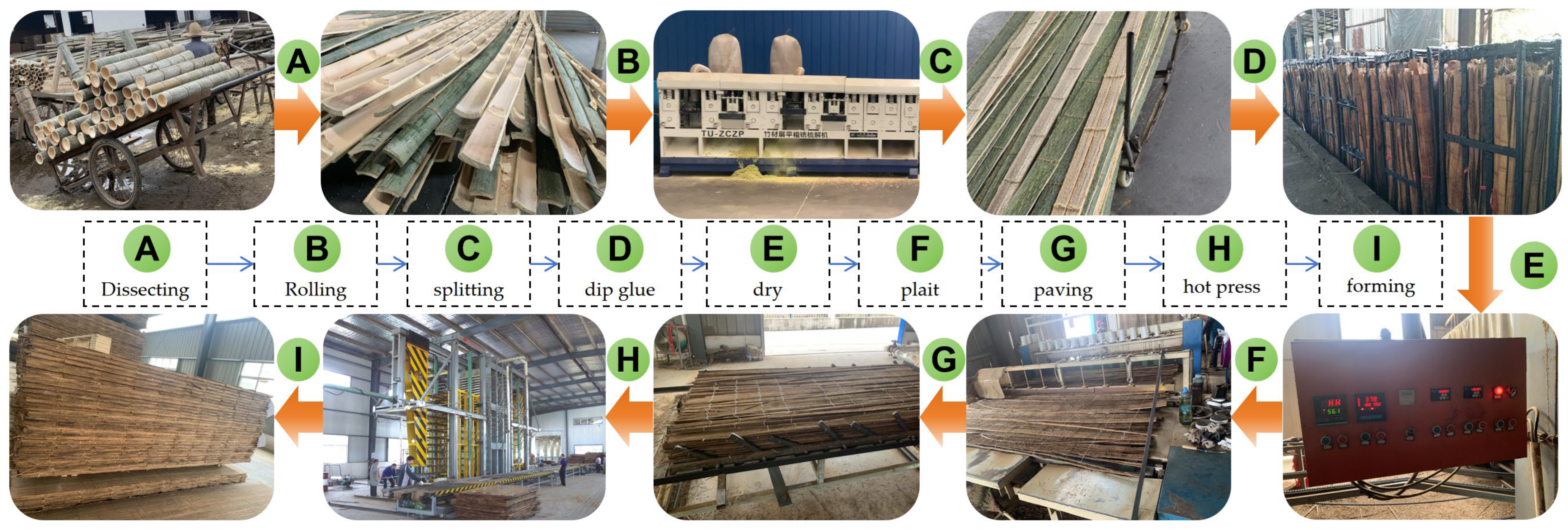
2.1. Materials

In the present investigation, a heavy-duty multilayer hot press designated for bamboo-based fiber composites (BY4×7-8/240(20), Qingdao Kokusen Machinery Company Limited, Qingdao City, China) was employed as the primary subject of study. The structural configuration of this press is presented in Figure 2a, outlining its critical parameters, such as the main cylinder’s 2400-ton pressure capacity, the 1400 × 2700 mm dimensions of the hot platen, the presence of 20 platen layers, the 250 mm size of the open gear, the utilization of a high-temperature steam-heating method, and its remarkable annual production capacity of up to 50,000 m³.

The multilayer hot press comprises three integral components: the main body, the control and drive system encompassing both the electric and hydraulic subsystems, and the heating system. Notably, this paper centers its attention on the intricate heating cycle system of this heavy-duty multilayer hot press. Within this system, a boiler functions as the generator of high-temperature saturated steam, which is then directed to the hot press via a sophisticated network of piping. Precise flow control is achieved through the utilization of a steam-regulating valve within this intricate piping network.

A steam-conditioning valve serves as a pivotal device in regulating steam flow, ensuring the precise adjustment of steam quantities traversing piping systems. This valve typically comprises a valve body, multiple valve seats, a valve flap (or spool), and an actuating mechanism such as an electric, pneumatic, or hydraulic actuator [16]. The operation of these valves is governed by a high-precision control system that responds dynamically to temperature sensor feedback within the hot press, thus maintaining a balanced and stable temperature across each layer. A schematic representation of the heating cycle system for a heavy-duty multilayer hot press is depicted in Figure 2b.

In Figure 2b, a clear correlation can be observed between the temperature of the heavy-duty multilayer hot press and the steam flow rate. Specifically, an increase in the steam flow rate corresponds to an elevation in the hot press’s temperature, and conversely, a reduction in the steam flow leads to a decrease in temperature. Furthermore, the steam flow is directly influenced by the opening angle of the steam-regulating valve. The methodology for establishing the transfer function between the opening angle of the steam-regulating valve and the temperature of the hot press is thoroughly elaborated in the subsequent sections of this study.

The dry-air density of the fibrotic bamboo veneer used in this study was 0.51 g/cm³, and the moisture content was 9.9%. The selected phenolic resin adhesive had a solid content of 52.5%, viscosity of 188 cp, and pH value of 10.22, and the curing temperature was 140 °C.

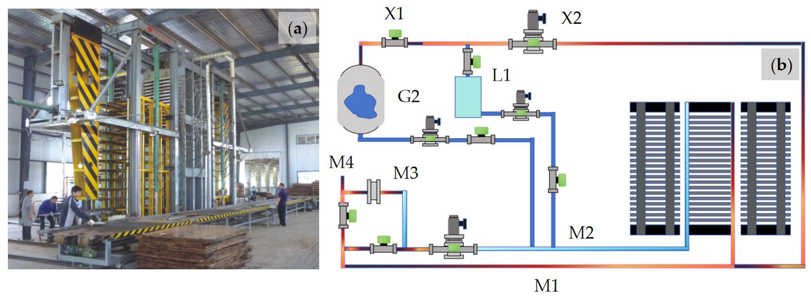
2.2. Modeling of Motor-Driven Steam Control Valve Opening Angle

From a rigorous analytical standpoint, a preceding investigation revealed that the opening angle of a motor-driven steam control valve has a direct influence on the flow rate of hot steam, which subsequently impacts the temperature [17]. Consequently, it becomes imperative to develop a model for the opening angle of the steam-regulating valve to facilitate a more precise characterization of the temperature dynamics. The regulating valve control system, as depicted in Figure 3, comprises crucial components such as an embedded controller, a valve drive system, a data processing unit, and a pressure sensor [18]. Once the desired flow rate is set in the logic-programmable controller, the opening angle controller acquires the real-time opening angle value of the valve and measures the pressure differential across the valve using a pressure sensor. These data are then transmitted to the upper computer, which utilizes interpolation calculations on the temperature data table to deduce the appropriate valve opening angle corresponding to the target temperature. This derived value is then relayed back to the opening angle controller, which generates a signal to adjust the valve’s opening angle. Subsequently, the controller transmits this signal to the valve drive system, instructing it to manipulate the valve to achieve the desired opening angle. During this process, the motor’s angular displacement is effectively transformed into linear displacement through a worm gear and screw mechanism, thereby enabling precise control of the valve’s opening angle [19].

Regarding the control signal generated by the PLC and subsequently converted by A/D to adjust the opening angle of the steam valve, this component is represented by a higher-order transfer function incorporating a delay element [20,21]. Nevertheless, the active disturbance rejection control inherent in this higher-order transfer function poses convergence challenges, making it difficult to attain the intended control effect. Upon closer examination of this higher-order transfer function, it becomes apparent that it can be simplified into multiple constant gain values. Furthermore, based on a practical analysis of the system’s behavior, it is reasonable to omit this component from further consideration.

2.3. Modeling of Steam-Regulating Valve Opening Angle in Terms of Heat, Pressure, and Temperature

The opening angle of the steam conditioning valve holds a direct influence on the flow rate of hot steam, subsequently impacting the temperature of the hot press via a heat transfer mechanism. The traditional generalized representation of the second-order transfer function pertaining to this phenomenon is presented in Equation (1):

$$G(s)=\frac{K•{\omega }_n^2}{s^2+2\zeta {\omega }_{n}s+{\omega }_n^2}$$

(1)

where ${\omega }_n$ is the natural frequency; and $\zeta$ is the damping ratio.

Conventional second-order systems have demonstrated their ability to model the oscillatory and transitional characteristics of a system. Nevertheless, acknowledging the inherent time lag associated with temperature changes, this study introduces novel modifications to the transfer function by incorporating an additional time delay term and an oscillation term. These enhancements aim to provide a more accurate representation of the system dynamics. The refined transfer function, incorporating these modifications, is presented in Equation (2):

$$G(s)=\frac{K_p}{(T_2{s}^2+T_{1}s+1)}{e}^{-T_{d}s}$$

(2)

where $K_p$ is the gain; $T_1$ is the first-order time constant; $T_d$ is the second-order time constant; and is the time delay.

During the heat transfer process between steam and a hot platen, the temperature change lacks a definitive analytical relationship. Consequently, the numerical solution is typically obtained through the finite element method. Therefore, in this study, we aimed to establish a correlation between the opening angle of the steam regulator valve and the temperature of the hot platen through the application of a parameter identification method.

The recursive least squares method represents an efficient algorithmic approach in the domain of dynamic system parameter identification. This method facilitates the continuous real-time updating and optimization of model parameters, given a known dynamic structure of the system [22]. The formula for recursive least squares parameter estimation is presented in Equation (3).

$$\left\{\begin{array}{l}{\widehat{\theta }}_{N+1}={\widehat{\theta }}_N+P_{N+1}{\phi }_{N+1}\left[y(N+1)-{\phi }_{N+1}^T{\widehat{\theta }}_N\right]\hfill \\ {\gamma }_{N+1}={(I+{\phi }_{N+1}^T{P}_N{\phi }_{N+1})}^{-1}\hfill \\ P_{N+1}=(I-K_{N+1}{\phi }_{N+1}^T)P_N\hfill \\ K_{N+1}={\gamma }_{N+1}{P}_N{\phi }_{N+1}\hfill \end{array}\right.$$

(3)

where ${\widehat{\theta }}_{N+1}$ is the updated value of the parameter estimate; ${\widehat{\theta }}_N$ is the parameter estimate; ${\phi }_N$ is the information vector; P is the bias term in the parameter estimates; and $y(N)$ is the system output.

Based on the aforementioned information, this study employed a recursive least squares method with a dynamic forgetting factor for the parameter identification of the model. The introduction of the dynamic forgetting factor enables the model to retain useful information while reducing the accumulation of errors caused by non-stationary behaviors, thus enhancing the model’s adaptability and sensitivity to new data. The performance indicator is defined as shown in Equation (4).

$$J={{\displaystyle \sum _{k=1}^N{\lambda }^{N-k}\left[y(k)-{\phi }^T(k)\widehat{\theta }\right]}}^2$$

(4)

By applying a time-varying coefficient to the data, the older data are weighted down, while the latest data are given more weight. Consequently, this approach is also referred to as the exponential forgetting algorithm. The recursive least squares parameter estimation method with a forgetting factor is presented in Equation (5).

$$\left\{\begin{array}{l}{\widehat{\theta }}_{N+1}={\widehat{\theta }}_N+P_{N+1}{\phi }_{N+1}\left[y(N+1)-{\phi }_{N+1}^T{\widehat{\theta }}_N\right]\hfill \\ {\gamma }_{N+1}={({\lambda }^2+{\phi }_{N+1}^T{P}_N{\phi }_{N+1})}^{-1}\hfill \\ P_{N+1}=\frac{1}{{\lambda }^2}(I-K_{N+1}{\phi }_{N+1}^T)P_N\hfill \\ K_{N+1}={\gamma }_{N+1}{P}_N{\phi }_{N+1}\hfill \end{array}\right.$$

(5)

where ${\widehat{\theta }}_{N+1}$ is the updated value of the parameter estimate; ${\widehat{\theta }}_N$ is the parameter estimate; ${\phi }_N$ is the information vector; λ is the forgetting factor; P is the bias term in the parameter estimates; and $y(N)$ is the system output.

The performance of the forgetting factor recursive least squares method hinges on the value of λ. When λ is excessively large, it can enhance the algorithm’s robustness to noise in observations, but it can compromise its tracking capability. Conversely, a too-small λ results in a faster tracking speed of the algorithm, yet it becomes more sensitive to noise, leading to a decrease in the accuracy of the parameter identification. Therefore, when designing the forgetting factor λ, a balance must be struck between the algorithmic precision and its noise resilience. The aforementioned forgetting factor recursive least squares method typically assumes a constant value for λ. However, if the forgetting factor λ is be adjusted in real time based on the proximity of the identification results to the actual system model, the algorithm will be less prone to impairment in terms of its identification accuracy and tracking ability caused by overly large or small λ values. This dynamic adjustment allows for the continuous optimization of the algorithm’s overall performance, significantly enhancing its parameter identification capabilities. The model’s residual at time k is given by Equation (6), as follows:

$$\mathrm{e}\left(k\right)=y(k)-\phi {\left(k\right)}^{\mathrm{T}}{\widehat{\theta }}_{k-1}$$

(6)

where $y(k)$ is the system output value at moment k, i.e., the measured value of the system; and $y(k)-\phi {\left(k\right)}^{\mathrm{T}}{\widehat{\theta }}_{k-1}$ is the estimated value.

The presence of residuals is primarily attributed to noise and identification errors, with noise having a relatively minor impact on them. When the error in the system parameter identification is significant, resulting in large absolute values of residuals, reducing the forgetting factor can enable the system’s identification results to quickly converge to parameters close to the actual model, thereby narrowing the convergence range. At this point, with smaller absolute values of residuals, increasing the forgetting factor can suppress the influence of noise on the identification results, ultimately enhancing the overall performance of the algorithm in system identification. To this end, an evaluation function is adopted, as defined in Equation (7):

$$J_{\mathrm{F}}=\frac{1}{\mathrm{M}}{\displaystyle \sum _{k=\mathrm{N}-\mathrm{M}}^{\mathrm{N}}\left|\mathrm{e}\left(k\right)\right|}$$

(7)

Since relying solely on the absolute value of a single residual to adjust the forgetting factor leads to low accuracy, the average of residuals over a certain period was chosen as a performance indicator for convergence to the actual parameter values during the identification process. However, this indicator exhibits an inverse correlation with the degree of correction applied to the forgetting factor, making it challenging to establish a mathematical expression between the two. Therefore, fuzzy control theory was introduced to design a fuzzy controller for online modification of the forgetting factor. The change rate after the Nth observation is given by Equation (8):

$$\Delta J_{\mathrm{F}}\left(\mathrm{N}\right)=\frac{1}{\mathrm{D}}\left(J_{\mathrm{F}}\left(\mathrm{N}\right)-J_{\mathrm{F}}(N-\mathrm{D})\right)$$

(8)

where D is the constant-time discrete value for calculating the rate of change in $J_{\mathrm{F}}$; and $J_{\mathrm{F}}$ and $\Delta J_{\mathrm{F}}$ are the inputs to the fuzzy controller.

The correction forgetting factor is shown in Equation (9):

$$\lambda ={\lambda }_0+\Delta \lambda$$

(9)

where ${\lambda }_0$ is the initial forgetting factor; $\Delta \lambda$ is the output of the fuzzy controller; and $\lambda$ is the updated value of the forgetting factor.

When employing the dynamic forgetting factor recursive least squares method, the correction period is designated as L times the sampling period, thus initializing the variation M to zero. Subsequently, the following steps are executed:

(1)

Prior to commencement, establish the initial parameter estimates, the initial covariance matrix, and the initial forgetting factor. Conventionally, the covariance matrix is initialized as a larger positive number multiplied by the unit matrix, indicating a high degree of initial uncertainty. The initial values of $\widehat{\theta }(0)$, $P(0)$, and ${\lambda }_0$ are set, and the initial data is entered accordingly.

(2)

Determine the ratio of the correction period $T_r$ to the sampling period $T_s$. This signifies that the parameter estimates will undergo an update following each sampling period.

(3)

Increment M by 1, collect the current input u(k) and output y(k), and compute the residual using Equation (6).

(4)

If M is less than L, repeat the previous step; otherwise, reset M to zero and proceed with the subsequent step.

(5)

Preprocess the data utilizing Equations (7) and (8) to derive the values of $J_{\mathrm{F}}$ and $\Delta J_{\mathrm{F}}$.

(6)

Input $J_{\mathrm{F}}$ and $\Delta J_{\mathrm{F}}$ into the fuzzy controller and determine C through control rule table reasoning.

(7)

Compute $\widehat{\theta }$, P, and K by applying Equation (9) to Equation (5). At this juncture, the identification of the single parameter is completed, and the process returns to the third part for the continuation of the cycle.

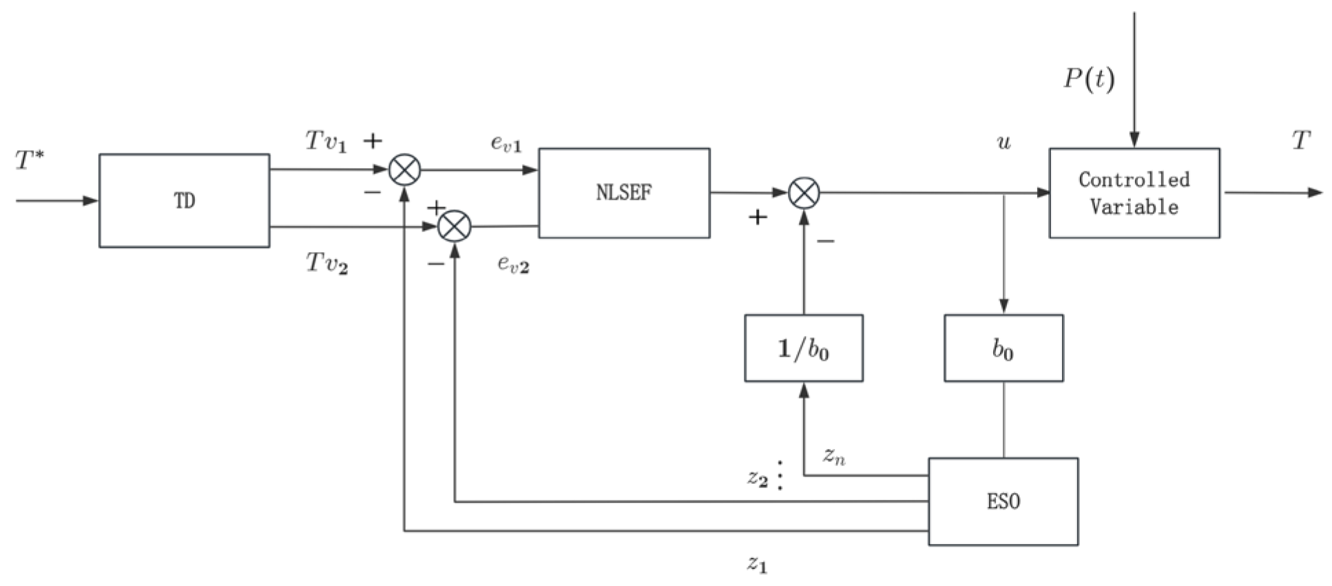
2.4. Design of ADRC

ADRC is a contemporary control methodology whose fundamental principle revolves around estimating and compensating for both internal and external system perturbations in real time to enhance the control performance [23]. The self-immobilizing controller comprises three integral components: the tracking differentiator (TD), the extended-state observer (ESO), and the nonlinear state error feedback mechanism. The TD facilitates a smooth transition process, accurately tracking the reference input signal T* and mitigating abrupt changes in T*. The ESO offers estimations of the system’s state variables, z₁ and z₂, as well as a real-time assessment of system perturbations. The nonlinear state error feedback converts the error between the transition process and the object’s state variables into a nonlinear combination, providing the necessary control input for the system [24]. These three components are interconnected, yet they can be designed independently. Figure 4 illustrates the basic structural configuration of this control architecture.

2.4.1. Tracking Differentiator

As an integral component of ADRC, the tracking differentiator enhances the system’s responsiveness and stability by delicately smoothing and filtering noise from the input signals, providing the controller with denoised and continuously differentiable signals [25]. This mechanism not only optimizes the quality of the control inputs, mitigating the adverse effects of measurement errors and external disturbances, but it also furnishes crucial dynamic information for the design of control laws. In dynamic processing environments, the presence of the tracking differentiator significantly elevates the adaptability of the temperature control system, enabling it to promptly and accurately reflect the actual conditions during the hot-pressing process of bamboo-based fiber composites and achieve precise temperature regulation.

Conventional differentiators typically approximate delay elements using first-order inertial links, yet they possess the limitation of amplifying random noise. Therefore, the classical differentiator was refined into a second-order nonlinear form, as depicted in Equation (10):

$$\left\{\begin{array}{l}{\dot{x}}_1=x_2\\ {\dot{x}}_2=-\mathrm{r} \mathrm{sgn}\left(x_1-\mathrm{v}\left(\mathrm{t}\right)+\frac{x_2\left|x_2\right|}{\mathrm{r}}\right)\end{array}\right.$$

(10)

${\dot{x}}_1=x_2$ signifies that the rate of change in the state quantity x₁ is equivalent to the state quantity x₂. In the context of a universal differentiator, x₁ denotes the position, while x₂ represents the velocity. The symbol ${\dot{x}}_2$ denotes the rate of change in x₂, expressed as a nonlinear function that depends on x₁ and the control input. The term -rsgn(x₁ − v(t)) serves as feedback to the error signal (x₁ − v(t)), where r is the gain coefficient, also known as the speed factor, which governs the tracking speed. The tracking speed is directly proportional to the value of r, resulting in an improved speed compared to the linear tracking differentiator. However, in cases where the input signal contains high-frequency noise, the output differential signal may still exhibit significant noise. The function sgn is utilized to determine the tracking speed based on the deviation from the target trajectory v(t), thereby dictating the direction of the feedback. $\frac{x_2\left|x_2\right|}{\mathrm{r}}$ introduces nonlinear damping to the state quantity x₂. The fastest tracking algorithm is incorporated into the nonlinear tracking differentiator, and the discretization of the aforementioned equation is presented in Equation (11):

$$\left\{\begin{array}{l}{x}_1\left(k+1\right)=x_1\left(k\right)+\mathrm{h}{x}_2\left(k\right)\\ x_2\left(k+1\right)=x_2\left(k\right)+\mathrm{hu},\left|\mathrm{u}\right|\le \mathrm{r}\end{array}\right.$$

(11)

where h is the step size, and the expression for u is shown in Equation (12):

$$\mathrm{u}=-r \mathrm{sgn}\left(x_1\left(k\right)-\mathrm{v}\left(k\right)+\frac{x_2\left(k\right)\left|x_2\left(k\right)\right|}{2\mathrm{r}}\right)$$

(12)

The introduction of the fhan function into the control law, as detailed in Equation (13), incorporates a crucial parameter a, which serves as an accuracy factor that dictates the precision of the differential operation.

$$\left\{\begin{array}{l}d=rh\\ d_0=hd\\ a_0=\sqrt{d^2+8r\left|y\right|}\\ a=\left\{\begin{array}{l}{x}_2+\frac{\left(a_0-d\right)}{2}\mathrm{sgn}\left(y\right),\left|y\right|>d_0\\ x_2+\frac{\mathrm{y}}{\mathrm{h}},\left|y\right|\le d_0\end{array}\right.\\ \mathrm{fhan}=-\left\{\begin{array}{l}\mathrm{r} \mathrm{sgn}\left(a\right),\left|a\right|>d\\ \mathrm{r}\frac{a}{d},\left|a\right|\le d_0\end{array}\right.\end{array}\right.$$

(13)

Then, the expression of the final tracking differentiator is shown in Equation (14):

$$\left\{\begin{array}{l}\mathrm{e}\left(k\right)=x_1\left(k\right)-v_1\left(k\right)\\ x_1\left(k+1\right)=x_1\left(k\right)+\mathrm{h}{v}_2\left(k\right)\\ x_2\left(k+1\right)=x_2\left(k\right)+\mathrm{hfhan}\left(\mathrm{e}\left(k\right),x_2\left(k\right),r,h_0\right)\end{array}\right.$$

(14)

where v₁ represents the tracking signal for the input ideal temperature signal v₀, while v₂ denotes the first-order tracking differential signal of v₀. The filtering factor is denoted by h₀. The fhan function comprises two adjustable parameters: r₀ and h₀. Specifically, r₀ serves as the speed factor, governing the tracking sensitivity of the TD (tracking differentiator) to the input signal, thus balancing the tracking speed and sensitivity. On the other hand, h0 functions as the filtering factor, acting as a noise suppression factor that influences both the sensitivity and smoothing capabilities of the TD. The convergence of the tracking differentiator is contingent upon the presence of a fixed point in the system, i.e., when v2(k) = 0 and certain conditions (denoted as $\mathrm{fhan}\left(\mathrm{e}\left(k\right),x_2\left(k\right),r,h_0\right)$) are satisfied. Additionally, the appropriate selection of the step size h and the favorable properties of the fhan function contribute to the convergence.

For the temperature control process in the hot-pressing molding of bamboo-based fiber composites, the tracking differentiator provides both the tracking signal and the first-order differential signal of the reference command signal. This effectively mitigates the discrepancy between the system’s response speed and the overshoot phenomenon that can arise from initial errors. Given the swiftness and accuracy of the tracking differentiator, Equations (13) and (14) are adopted to design the tracking differentiator for the temperature control process.

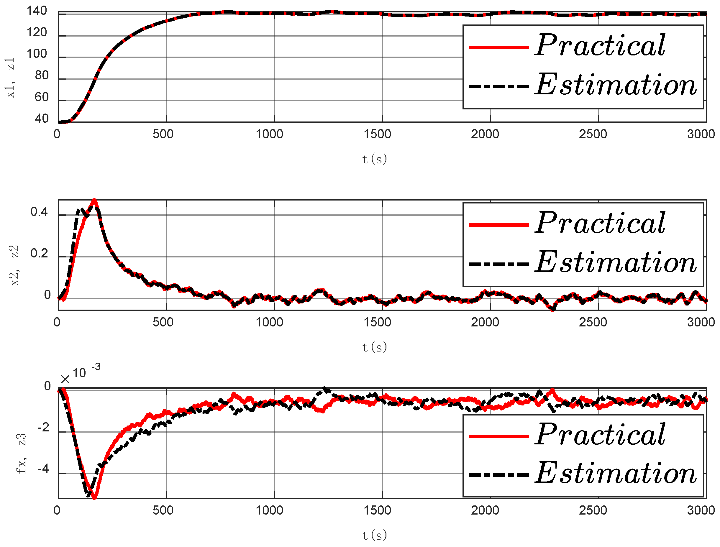
2.4.2. Expanded State Observer

The expanded state observer (ESO) serves as a pioneering state estimator in active disturbance rejection control systems, underpinned by its design philosophy of real-time estimation of comprehensive state information pertaining to the control object. This estimation encompasses the system’s response to both internal dynamics and external perturbations. The ESO’s introduction is particularly apt for control scenarios where model accuracy is constrained or system parameters undergo significant variations, a prime example being the hot-compression molding process of bamboo-based fiber composites [26]. In this process, temperature control holds a pivotal role in determining the overall product quality.

Within the temperature control system for the hot-pressing molding of bamboo-based fiber composites, the total disturbance, denoted as d, is treated as an unknown state variable. Based on the existing state variables of the original system, a new state is introduced, as exemplified in Equation (15).

$$\left\{\begin{array}{l}{\dot{x}}_1=x_2=\dot{T}\\ {\dot{x}}_2=d+bu\\ {\dot{x}}_3=\dot{d}\\ y=x_1\end{array}\right.$$

(15)

To this expanded linear system, a nonlinear state observer is constructed, as presented in Equation (16), ensuring a robust and precise estimation of the system’s dynamics.

$$\left\{\begin{array}{l}{\epsilon }_1=z_1-y\\ {\dot{z}}_1=z_2-{\beta }_{01}{\epsilon }_1\\ {\dot{z}}_2=z_3-{\beta }_{02}fal\left({\epsilon }_1,{\alpha }_1,\delta \right)+b_{0}u\\ {\dot{z}}_3=-{\beta }_{03}fal\left({\epsilon }_1,{\alpha }_1,\delta \right)\end{array}\right.$$

(16)

In the context of the equation given above, z₁ and z₂ represent the observed values of the state variables x₁ and x₂, while z₃ denotes the observed value of the total system disturbance. The parameters ${\alpha }_1$, $\delta$, ${\beta }_{01}$, ${\beta }_{02}$, ${\beta }_{03}$, and E serve as tunable coefficients within the framework. It is noteworthy that the parameters ${\alpha }_1$ and $\delta$ exhibit a mutual coupling effect on the overall system performance. The tuning process of ${\beta }_{01}$, ${\beta }_{02}$, and ${\beta }_{03}$ can be effectively transformed into a bandwidth tuning problem, which involves adjusting the controller’s bandwidth to achieve desirable dynamic performance. The nonlinear function, as represented in Equation (17), plays a crucial role in estimating the state variables and the total perturbation scenario in a real-time and rapid manner.

$$fal\left({\epsilon }_{\mathrm{i}},{\alpha }_{\mathrm{i}},\delta \right)=\left\{\begin{array}{l}{\left|{\epsilon }_{\mathrm{i}}\right|}^{{\alpha }_{\mathrm{i}}}\mathrm{sgn}\left({\epsilon }_{\mathrm{i}}\right),\left|{\epsilon }_{\mathrm{i}}\right|>\delta \\ \frac{{\epsilon }_{\mathrm{i}}}{{\delta }^{1-{\alpha }_{\mathrm{i}}}},\left|{\epsilon }_{\mathrm{i}}\right|\le \delta ,\delta >0\end{array}\right.$$

(17)

Specifically, when the error is significant, a nonlinear feedback ${\left|{\epsilon }_{\mathrm{i}}\right|}^{{\alpha }_{\mathrm{i}}}\mathrm{sgn}\left({\epsilon }_{\mathrm{i}}\right)$ is provided, whereas under small error conditions, a linear feedback $\frac{{\epsilon }_{\mathrm{i}}}{{\delta }^{1-{\alpha }_{\mathrm{i}}}}$ is employed. This strategy ensures that the error gradually decreases over time and ultimately converges to zero, thereby facilitating the convergence of the state observer.

2.4.3. Nonlinear State Error Feedback

Nonlinear state error feedback assumes a pivotal role in managing systems with intricate dynamic characteristics. Specifically, nonlinear functions are leveraged to devise a feedback control law for state errors, aiming to bolster the system’s robustness against a diverse array of operating conditions and perturbations [27]. The crux of this approach lies in the design of the nonlinear function, which must aptly capture the magnitude and direction of the error, offer suitable control effects, and adapt to the system’s nonlinear characteristics across various operating regions [28]. The state error is expressed in Equation (18):

$$\begin{array}{l}{\mathrm{e}}_1={\mathrm{v}}_1-{\mathrm{z}}_1\\ {\mathrm{e}}_2={\mathrm{v}}_2-{\mathrm{z}}_2\end{array}$$

(18)

where e₁ and e₂ represent the state errors; v₁ is the tracking signal for the reference input signal; v₂ denotes the differential signal of the tracking signal; and z₁ and z₂ are the state outputs of the state observer.

Subsequently, by combining e₁ and e₂, the expansion state quantities are compensated using an independent nonlinear method. This nonlinear combination is formulated in Equation (19), ensuring a precise and adaptive control response to the system’s dynamic behavior.

$${\mathrm{u}}_0={\beta }_{1}fal\left({\mathrm{e}}_1,{\alpha }_1,\delta \right)+{\beta }_{2}fal\left({\mathrm{e}}_2,{\alpha }_2,\delta \right)$$

(19)

The nonlinear function serves as the cornerstone of the nonlinear state error feedback mechanism [29]. It typically exhibits a segmented definition, wherein the gain of the control law is modulated in diverse manners based on the error magnitude, thereby enabling precise regulation of the ${\beta }_{1}fal\left({\mathrm{e}}_1,{\alpha }_1,\delta \right)$ system’s state. When the error surpasses a predetermined threshold $\delta$, the fal() function manifests as a symbolic function of e₁, and the control system incorporates a hard saturation feature to guarantee a robust response to significant deviations. Conversely, for errors below the threshold, the function assumes a form proportional to e₁ and ${\alpha }_1$, ensuring a smooth and continuous control action that avoids over-amplification in scenarios of minor errors. This approach leverages the mathematical advantage of “large error, small gain; small error, large gain”, reducing the steady-state duration of high-frequency oscillations while exhibiting a simple structure, high control efficiency, and robust characteristics [30]. Within the given formulation, the parameters α₁, $\delta$, ${\beta }_1$, ${\beta }_2$, α₂, and $\delta$ require adjustment. These parameters exhibit a mutual coupling effect on the system’s performance, and ${\beta }_1$ and ${\beta }_2$ can be fine-tuned using bandwidth-based methods.

The nonlinear regulation mechanism assumes paramount importance in the temperature control of hot-pressing molding for bamboo-based fiber composites [31]. Specifically, the fal() function empowers the control system to provide apt control inputs under diverse operating conditions, encompassing rapid temperature gradient changes and external perturbations [32]. By optimizing the control strategy, the hot-pressing temperature can be stabilized within an optimal range, thereby ensuring the consistency and stability of the processing quality for bamboo-based fiber composites. The intermediate control law u₀ and the extended state z₃ collectively constitute the final control law, as depicted in Equation (20).

$$\mathrm{u}=\frac{{\mathrm{u}}_0-{\mathrm{z}}_3}{{\mathrm{b}}_0}$$

(20)

Equation (21) can be obtained from Equation (18):

$$\begin{array}{l}{\stackrel{·}{\mathrm{e}}}_1={\mathrm{v}}_1-{\stackrel{·}{\mathrm{z}}}_1\\ {\stackrel{·}{\mathrm{e}}}_2={\mathrm{v}}_2-{\stackrel{·}{\mathrm{z}}}_2\end{array}$$

(21)

The Lyapunov function V(e) is chosen, as shown in Equation (22):

$$\mathrm{V}\left(\mathrm{e}\right)=\frac{1}{2}{{\mathrm{e}}_1}^2+\frac{1}{2}{{\mathrm{e}}_2}^2$$

(22)

The time derivative of V(e) is shown in Equation (23):

$$\stackrel{·}{\mathrm{V}}\left(\mathrm{e}\right)={\mathrm{e}}_1{\stackrel{·}{\mathrm{e}}}_1{+\mathrm{e}}_2{\stackrel{·}{\mathrm{e}}}_2$$

(23)

Substituting Equation (21) into Equation (23) yields Equation (24)

$$\stackrel{·}{\mathrm{V}}\left(\mathrm{e}\right)={\mathrm{e}}_1\left({\mathrm{v}}_1-{\stackrel{·}{\mathrm{z}}}_1\right){+\mathrm{e}}_2\left({\mathrm{v}}_2-{\stackrel{·}{\mathrm{z}}}_2\right)$$

(24)

The error dynamics are expressed in terms of a nonlinear feedback term, and the result is shown in Equation (25):

$$\begin{array}{l}{\stackrel{·}{\mathrm{z}}}_1={\beta }_{1}fal\left({\mathrm{e}}_1,{\alpha }_1,\delta \right)\\ {\stackrel{·}{\mathrm{z}}}_2={\beta }_{2}fal\left({\mathrm{e}}_2,{\alpha }_2,\delta \right)\end{array}$$

(25)

Substituting Equation (25) into Equation (24) yields Equation (26):

$$\stackrel{·}{\mathrm{V}}\left(\mathrm{e}\right)={\mathrm{e}}_1\left({\mathrm{v}}_1-{\beta }_{1}fal\left({\mathrm{e}}_1,{\alpha }_1,\delta \right)\right){+\mathrm{e}}_2\left({\mathrm{v}}_2-{\beta }_{2}fal\left({\mathrm{e}}_2,{\alpha }_2,\delta \right)\right)$$

(26)

By adjusting α₁, $\delta$, ${\beta }_1$, ${\beta }_2$, α₂, and $\delta$ appropriately to ensure that the time derivative of the Lyapunov function is negative, Equation (27) is satisfied as follows:

$$\stackrel{·}{\mathrm{V}}\left(\mathrm{e}\right)<0,\forall \mathrm{e}\ne 0$$

(27)

When the error magnitude is significant, the function $fal\left({\mathrm{e}}_1,{\alpha }_1,\delta \right)$ introduces a smaller gain to mitigate excessive system responses, thus enhancing stability. Conversely, in scenarios where the error is minimal, $fal\left({\mathrm{e}}_1,{\alpha }_1,\delta \right)$ offers a higher gain to expedite the rapid convergence of the error towards zero, further enhancing system stability. This approach ensures that the system remains robust and stable across a diverse range of operating conditions, with the error asymptotically converging to zero, thereby affirming the stability of the overall system.

3. Results and Discussion

3.1. Parameter Identification Results for Steam Regulator Valve in Terms of Heat, Pressure, and Temperature Models

A comprehensive parameter identification test was conducted at Aoda Plywood Co. in Renhua County, Guangzhou City, Guangdong Province, China. The test duration spanned 2334 s, capturing crucial data throughout the entire thermal cycle of the bamboo-based fiber composite hot-pressing boards, starting from an ambient temperature of 27 °C and escalating to 140 °C. Selected outcomes of this test are presented in

Table 2. Selected data collected by the temperature control system.

Time (s)	Temp (°C)	Opening Angle	Flux (L/s)	Time (s)	Temp (°C)	Opening Angle	Flux (L/s)	Time (s)	Temp (°C)	Opening Angle	Flux (L/s)
47	50	0.994	151.18	93	82.5	0.788	119.91	940	140	0.0612	9.302
48	51	0.989	150.44	94	84	0.784	119.29	941	140	0.0612	9.312
49	51	0.984	149.69	95	86.2	0.780	118.68	942	140	0.0613	9.323
50	52	0.979	148.95	96	86.3	0.776	118.07	943	140	0.0614	9.334
51	52.1	0.975	148.22	97	86.4	0.772	117.46	944	140.1	0.0614	9.345
52	52.2	0.970	147.48	98	87.7	0.768	116.86	945	140.1	0.0615	9.357
53	53	0.965	146.75	99	87.9	0.764	116.26	946	140.1	0.0616	9.369
54	54	0.960	146.03	100	89.6	0.760	115.66	947	140.1	0.0617	9.380
55	55	0.955	145.30	101	89.6	0.757	115.06	948	140.1	0.0617	9.393
56	56.1	0.951	144.58	102	89.8	0.753	114.47	949	140.2	0.0618	9.405
57	56.2	0.946	143.86	103	89.8	0.749	113.88	950	140.2	0.0619	9.418
58	58.2	0.941	143.15	104	89.8	0.745	113.29	951	140.2	0.0620	9.431
59	58.3	0.937	142.43	105	90.9	0.741	112.71	952	140.2	0.0621	9.444
60	59.8	0.932	141.73	106	91	0.737	112.12	953	140.2	0.0622	9.457
61	59.9	0.927	141.02	107	92.2	0.733	111.54	954	140.1	0.0623	9.471

.

For the temperature control model of bamboo-based fiber composite hot-compression molding, focused on a second-order system, we employed industry-standard control logic to adjust the steam-regulating valve opening, thereby altering the hot-pressing temperature. Leveraging the forgetting factor recursive least squares method for parameter identification of the test data, we obtained the values of the identified parameters as $K_p$ = 0.67, $T_1$ = 1.055, $T_2$ = 100, and $T_d$ = 20 s. Consequently, the transfer function between the steam-regulating valve opening and the hot-pressing temperature was formulated as depicted in Equation (28):

$$G\left(s\right)=\frac{0.67}{100s^2+1.055s+0.00055}\cdot e^{-20s}$$

(28)

To facilitate the analysis, the aforementioned transfer function was reformulated into a state-space representation, yielding a mathematical model of the temperature control process, as shown in Equation (30):

$$\left\{\begin{array}{l}{\dot{x}}_1=x_2\\ {\dot{x}}_2=f\left(x_1,x_2\right)+bu+\omega \\ y=x_1\end{array}\right.$$

(29)

where $f\left(x_1,x_2\right)$ is (−T₁x₁ − T₂x₂); x₁ represents the apparent temperature of the hot press; x₂ is the rate of change in the apparent temperature of the hot press; $\omega$ encapsulates the system’s uncertainty and external perturbations; and b is the controller function.

The result of parameter identification shows that $\mathrm{b}=0.0067$, ${\mathrm{T}}_1=0.0000055$, and ${\mathrm{T}}_2=0.01055$. Then, $f\left(x_1,x_2\right)$ is shown in Equation (30):

$$f\left(x_1,x_2\right)=-0.0000055x_1-0.01055x_2$$

(30)

3.2. ADRC Parameterization Results

Parameter selection is a crucial aspect in the design of an auto-disturbance control system (ADRC), and these parameters directly determine the performance of the control system, including the response speed, accuracy, and robustness [33]. Suitable parameters can ensure the effective suppression of the system against external disturbances and internal dynamic changes [34]. Through the combination of theoretical analysis and experimental verification, the precise adjustment of the ADRC parameters plays an important role in improving the overall performance of the system. After testing each parameter individually, the parameter tuning results of the ADRC are shown in

Table 3. ADRC parameterization results.

Model	Parameter	Value
TD	$r$	100
	$h$	0.1
ESO	$\delta$	0.2
	${\alpha }_1$	0.25
	${\alpha }_2$	0.5
	${\beta }_{01}$	0.12
	${\beta }_{02}$	0.0048
	${\beta }_{03}$	0.0000512
NLSEF	${\dot{\alpha }}_1$	0.75
	${\dot{\alpha }}_2$	1.05
	${\beta }_1$	5
	${\beta }_2$	0.05
	$b_0$	0.0067

below, when the requirements of a higher response speed, lower overshoot, lower steady-state noise, and lower high-frequency vibration were guaranteed at the same time.

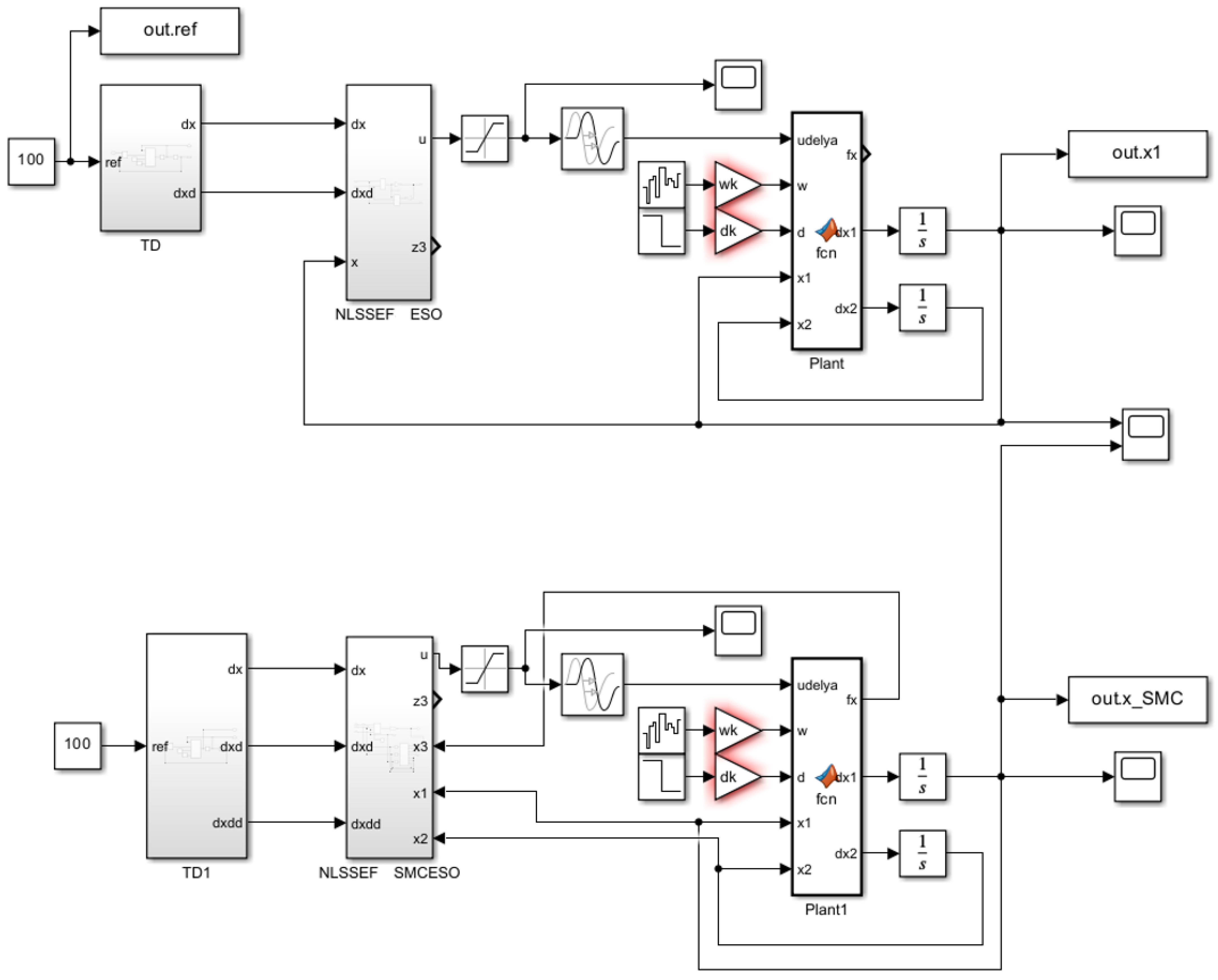
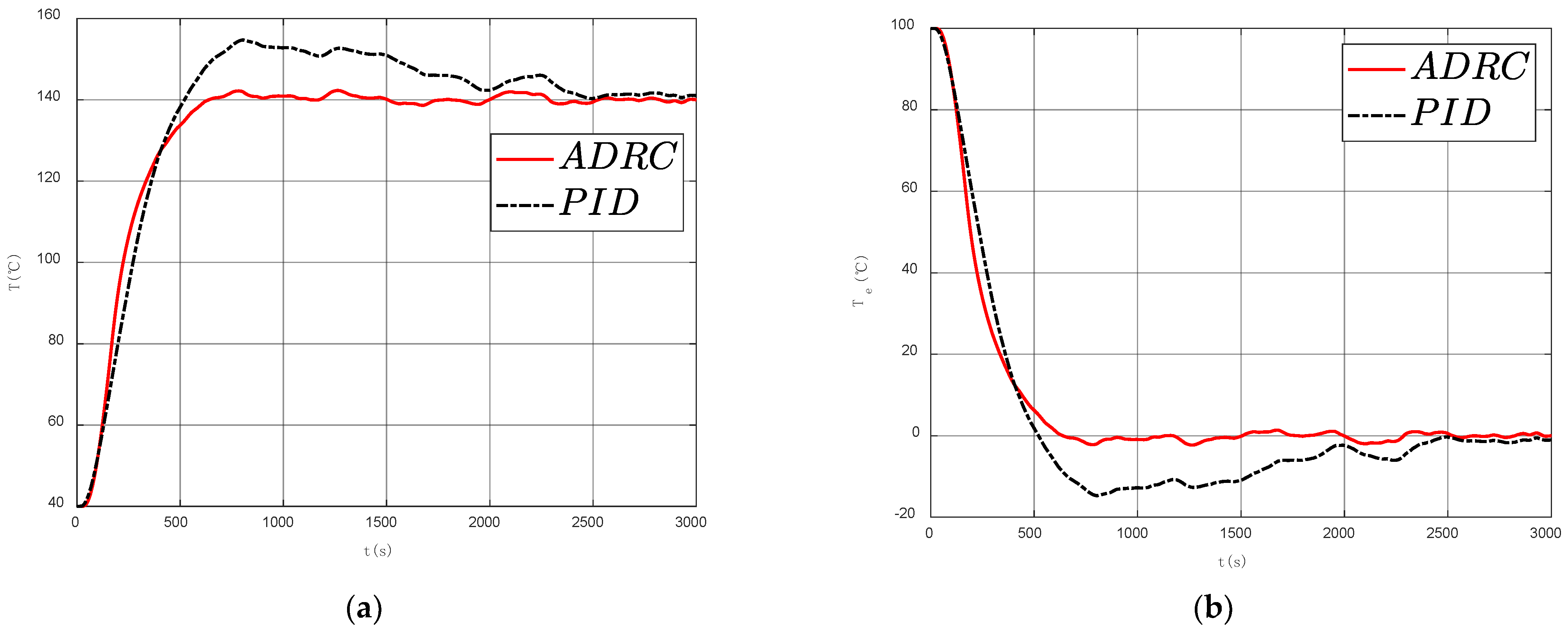
3.3. Simulation of ADRC of Hot-Compression Molding Temperature

Utilizing Matlab, a simulation model for the self-immunity-based temperature control system of bamboo-based fiber composite thermoforming was developed. This model facilitates the comparative simulation analysis of the control performance in response to uncertainties in the parameters of the bamboo-based fiber composite thermoforming temperature regulation model and the disturbances stemming from variations in heat conduction as well as measurement noise. A schematic of the temperature control system for the hot-pressing molding of bamboo-based fiber composites is presented in Figure 5, while the key parameters pertaining to the control object are summarized in

Table 4. Model input parameters for thermocompression temperature control system.

Model	Parameter	Value	Unit
Spool diameter	$D_1$	125	mm
Rated flow coefficient	$K_V$	200	-
Nominal pressure	$P_N$	6.4	MPa
Rated stroke	$S_1$	60	mm
Upper temperature limit	$T_m$	200	℃
Feedback position	$A_1$	20	mA
Rated power	$W_1$	2.5	kW
Rated voltage	$U_1$	380	V

.

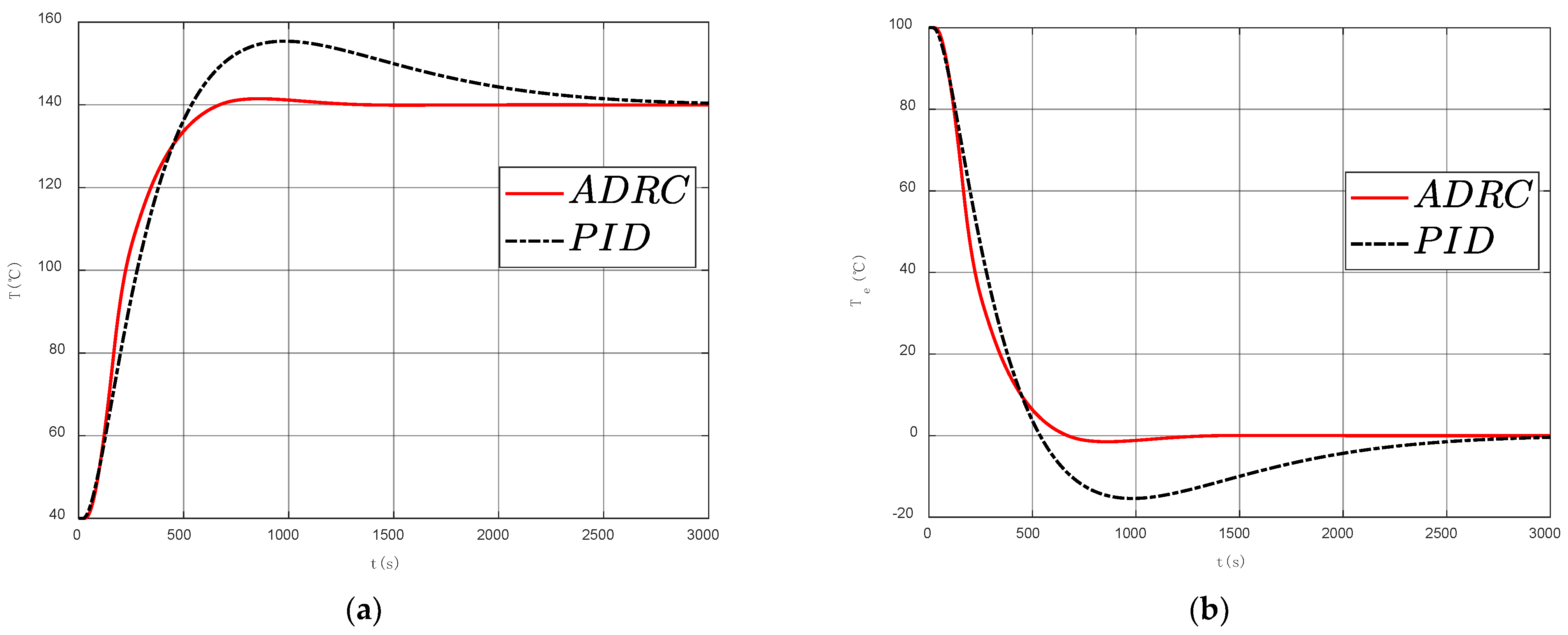
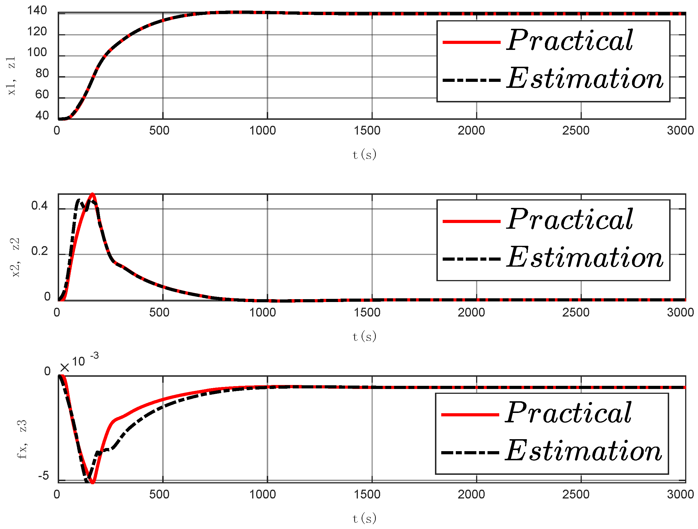
3.3.1. Simulation Results without Signal Interference

Drawing from the simulation structure diagrams presented in Table 3 and Table 4 and Figure 5, the solution-derived simulation results are depicted in Figure 6. As evident from the figure, the traditional PID temperature control system for the heavy-duty multilayer hot pressing of bamboo-based fiber composites exhibited significant overshoot above 140 °C, followed by slow cooling, ultimately returning to 140 °C. In contrast, the proposed ADRC (active disturbance rejection control) control strategy tailored specifically for the hot-pressing process of bamboo-based fiber composites commenced with an initial acceleration of the rate of temperature increase, enabling an earlier entry into the stabilization period while maintaining a constant 140 °C, thus achieving precise temperature regulation. Extensive testing of the bamboo-based fiber composite hot-pressing molding process revealed that the hot-pressing temperature was critical to ensuring product quality. When the temperature exceeded the set value, the phenolic resin adhesive curing accelerated, leading to premature curing of the surface layer. This, in turn, hindered the smooth release of internal steam, resulting in a “boiler effect” within the composite and the likelihood of a “burst board” phenomenon. Moreover, the pressure-holding process required a stable temperature of 140 °C. Significant temperature fluctuations during this phase could compromise heat transfer and reduce the adhesive curing speed, leaving internal reactions incomplete upon reaching the cooling stage. This led to an excessive internal moisture content and suboptimal physical and mechanical properties of the board. The simulation results demonstrated that the ADRC algorithm effectively mitigated these issues, ensuring stable and precise temperature control throughout the hot-pressing process.

The state estimation provided by the ESO is illustrated in Figure 7. Evidently, the expanded state observer, constructed utilizing the fal function, demonstrated the capability of smoothly and precisely estimating the state while simultaneously compensating for the control law, thereby fulfilling the necessary process requirements.

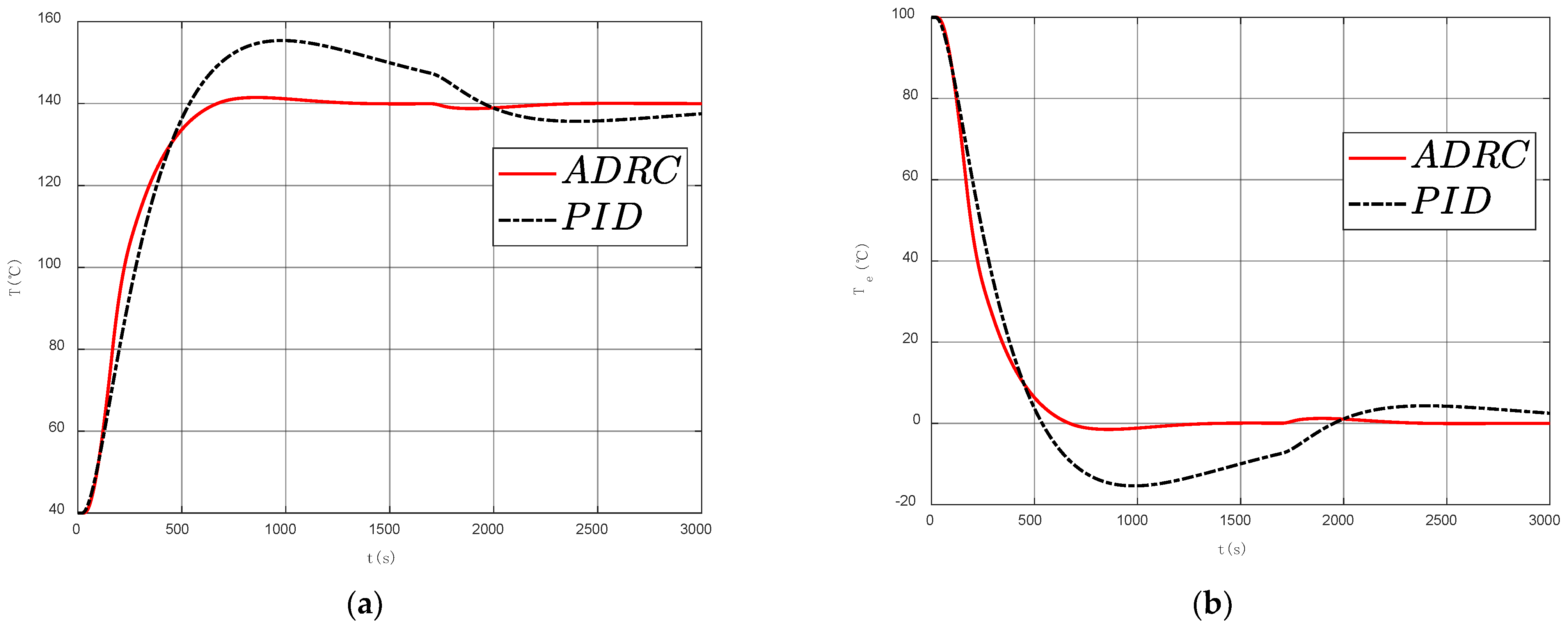
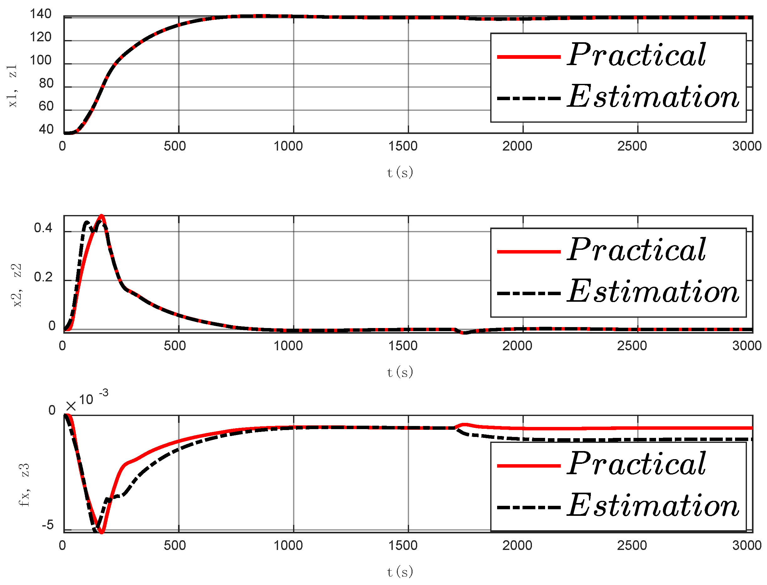
3.3.2. Simulation Results under Sinusoidal Signal Noise Interference

A sinusoidal disturbance signal was integrated into the system, and the controller parameters were optimized offline. The resulting simulation outcomes are depicted in Figure 8. Upon the introduction of the steam pressure pulsation interference simulation signal, the traditional PID control exhibited jittering during the cooling phase, preventing the temperature from stabilizing and thereby compromising the quality of the plate after the hot-pressing molding. Conversely, the ADRC controller, though exhibiting a minor jitter amplitude under a step response, remained unaffected in terms of its subsequent performance.

The state estimation of the ESO is presented in Figure 9. It becomes evident that the expanded state observer, formulated with the fal function, smoothly and precisely estimated the system state. This, coupled with the compensatory role of the control law, effectively achieved the objective of interference mitigation.

3.3.3. Simulation Results under Random Signal Noise Interference

In engineering applications, measurement noise is an inevitable challenge that often results in unnecessary production waste. Therefore, the mitigation of noise interference is a matter of significant concern within the engineering community. To emulate the impact of measurement noise within a narrow range of fluctuations around the desired value amidst random noise signals, we opted to compare the previously designed ADRC and PID controllers in terms of their output performance and error metrics. The simulation results, presented in Figure 10, reveal that under the influence of noise interference, the ADRC controller was capable of maintaining a stable output temperature at the desired value, exhibiting no overshoot and a smooth rise. Conversely, the PID controller failed to effectively mitigate the effects of measurement noise, resulting in noticeable errors. Although the ADRC exhibited some oscillations at steady-state temperatures, these were significantly reduced compared to the traditional PID controller.

Figure 11 depicts the state estimation performance of the ESO. It is evident that the expanded state observer, formulated with the fal function, provided a smoother and more accurate state estimation compared to the PID approach. Coupled with the compensatory role of the control law, the ESO-based approach achieved superior interference mitigation compared to the PID controller.

In summary, the differential tracker facilitated a smooth transition to the desired temperature, while the combined effect of the expanded state observer and the nonlinear state error feedback control law ensured robust resistance to external load perturbations. This combination resulted in an enhanced control effect for the hot-pressing temperature rise. When compared to the traditional PID control system, the ADRC control system demonstrated superior anti-interference performance for the temperature control of the hot-pressing molding of bamboo-based fiber composites.

4. Conclusions

In this study, an active disturbance rejection control (ADRC) method tailored for the thermoforming temperature regulation of bamboo-based fiber composites is proposed. Our findings indicate that in the absence of signal disturbances, the ADRC method significantly reduced the overshoot by approximately 87% compared to the traditional PID algorithm while concurrently shortening the time to achieve a steady state by about 58%. In scenarios involving sinusoidal signal disturbances, the ADRC method achieved a similar reduction in overshoot, approximately 85%, and expedited the stabilization process by roughly 49%. Notably, even in the presence of random signal disturbances, the ADRC method demonstrated remarkable performance, reducing the overshoot by approximately 74% and shortening the stabilization time by approximately 70%. The mathematical model established in this research, when coupled with the ADRC algorithm, exhibits exceptional efficiency and reliability. It is evident that this approach offers distinct advantages over the traditional PID algorithm in the precise control of thermoforming temperatures for bamboo-based fiber composites. Consequently, this study holds practical significance in enhancing the final product quality of bamboo-based fiber composites.

Compared to PID control, the ADRC control strategy can adaptively adjust the control parameters to respond to changes in the production environment and fluctuations in equipment performance through precise modeling and real-time disturbance estimation, effectively handling and resisting various internal and external disturbances. Therefore, the ADRC control strategy is more suitable for dynamic and ever-changing industrial environments. Meanwhile, using recursive least squares and the dynamic forgetting factor to solve the transfer function of industrial systems is more reasonable. However, although such a complex system and control mechanism can theoretically bring better hot-pressing temperature control, it may bring certain challenges in terms of its practical implementation and real-time performance. Specifically, there is also a high demand for computing resources and professional technical support, and management and maintenance costs and operational complexity increase linearly. How to adopt appropriate methods and allocate resources reasonably to solve the above problems and how better apply complex control systems and mechanisms to the industrial control of hot-pressing bamboo-based fiber composite materials are the subjects that this team will continue to research in the future.

References

1. De, B.; Bera, M.; Bhattacharjee, D.; Ray, B.C.; Mukherjee, S. A comprehensive review on fiber-reinforced polymer composites: Raw materials to applications, recycling, and waste management. Prog. Mater. Sci. 2024, 146, 101326. [Google Scholar] [CrossRef]
2. Kim, G.; Lee, H.; Arnold, K.; Rodriguez, J. Reusing uncured Fiber-reinforced thermoset composite Prepreg waste with water-soluble PVA backing film. Sustain. Mater. Technol. 2024, 41, e01016. [Google Scholar] [CrossRef]
3. Liu, L.; Xiang, D.; Ma, J.; Sun, H.; Harkin-Jones, E.; Wang, M.; Zeng, S.; Wu, Y. Multifunctional basalt fiber reinforced polymer composites with in-situ damage self-sensing and temperature-sensitive behavior. Compos. Commun. 2024, 101990. [Google Scholar] [CrossRef]
4. Xia, C.; Xie, W.; Meng, S.; Gao, B.; Ye, J. Preparation of integrated carbon fiber stitched fabric reinforced (SiBCN) ceramic/resin double-layered composites for ablation resistance, thermal insulation and compression resistance performance. Compos. Sci. Technol. 2024, 252, 110629. [Google Scholar] [CrossRef]
5. Shu, B.; Zhang, W.; Tao, Y.; Li, C.; Zhang, S.; Xiao, Z.; Fu, N.; Yu, J.; Gu, Y.; Lu, X. Mechanical Properties and Strength Design Value of Bamboo Scrimber. J. Northwest For. Univ. 2022, 37, 216–222. [Google Scholar]
6. Xu, D.; He, S.; Leng, W.; Chen, Y.; Wu, Z. Replacing Plastic with Bamboo: A Review of the Properties and Green Applications of Bamboo-Fiber-Reinforced Polymer Composites. Polymers 2023, 15, 4276. [Google Scholar] [CrossRef] [PubMed]
7. Qi, R.; Li, J.; Lin, J.; Song, Y.; Wang, J.; Cui, Q.; Qiu, Y.; Tang, M.; Wang, J. Design of the PID temperature controller for an alkaline electrolysis system with time delays. Int. J. Hydrog. Energy 2023, 48, 19008–19021. [Google Scholar] [CrossRef]
8. Liu, Z.; Liu, Z.; Liu, J.; Wang, N. Thermal management with fast temperature convergence based on optimized fuzzy PID algorithm for electric vehicle battery. Appl. Energy 2023, 352, 121936. [Google Scholar] [CrossRef]
9. Taler, D.; Sobota, T.; Jaremkiewicz, M.; Taler, J. Control of the temperature in the hot liquid tank by using a digital PID controller considering the random errors of the thermometer indications. Energy 2022, 239, 122771. [Google Scholar] [CrossRef]
10. Hou, G.; Gong, L.; Wang, M.; Yu, X.; Yang, Z.; Mou, X. A novel linear active disturbance rejection controller for main steam temperature control based on the simultaneous heat transfer search. ISA Trans. 2022, 122, 357–370. [Google Scholar] [CrossRef]
11. Dai, C.; Xue, Y.; Wu, Z.; Yan, G.; Li, D.; Li, Z. Active disturbance rejection control for the reheated steam temperature of a double-reheat boiler. J. Process Control 2023, 130, 103078. [Google Scholar] [CrossRef]
12. Liu, S.; Huang, H.; Li, D.; Tian, B.; Xue, W.; Sun, L.; Zhu, M. A hybrid receding horizon optimization and active disturbance rejection control of boiler superheated steam temperature. Process Saf. Environ. Prot. 2023, 178, 1107–1118. [Google Scholar] [CrossRef]
13. Li, Z.; Liang, S.; Guo, M.; Zhang, H.; Wang, H.; Li, Z.; Li, H. ADRC-Based Underwater Navigation Control and Parameter Tuning of an Amphibious Multirotor Vehicle. IEEE J. Ocean. Eng. 2024, 13, 4900. [Google Scholar] [CrossRef]
14. Gong, R.; Sun, R.; Chen, W. Series Active Disturbance Rejection Autopilot Design for Hyper Velocity Projectiles. IEEE Access 2020, 8, 149447–149455. [Google Scholar] [CrossRef]
15. He, D.; Li, Y.; Meng, X.; Si, Q. Anti-slip Control for Unmanned Underwater Tracked Bulldozer Based on Active Disturbance Rejection Control. Mechatronics 2022, 84, 102803. [Google Scholar] [CrossRef]
16. Pu, C.; Wang, Z.; Wang, S. Two-stage Active Disturbance Rejection Control for Coupled Permanent Magnet Synchronous Motors System With Mismatched Disturbance. Int. J. Control Autom. Syst. 2024, 22, 1883–1892. [Google Scholar] [CrossRef]
17. Cao, Y.; Cao, Z.; Feng, F.; Xie, L. ADRC-Based Trajectory Tracking Control for a Planar Continuum Robot. J. Intell. Robot. Syst. 2023, 108, 1. [Google Scholar] [CrossRef]
18. Zhang, J.; Cui, C.; Gu, S.; Wang, T.; Zhao, L. Trajectory Tracking Control of Pneumatic Servo System: A Variable Gain ADRC Approach. IEEE Trans. Cybern. 2023, 53, 6977–6986. [Google Scholar] [CrossRef]
19. Fang, Q.; Zhou, Y.; Ma, S.; Zhang, C.; Wang, Y.; Huangfu, H. Electromechanical Actuator Servo Control Technology Based on Active Disturbance Rejection Control. Electronics 2023, 12, 1934. [Google Scholar] [CrossRef]
20. Liu, C.; Luo, G.; Chen, Z.; Tu, W.; Qiu, C. A linear ADRC-based robust high-dynamic double-loop servo system for aircraft electro-mechanical actuators. Chin. J. Aeronaut. 2019, 32, 2174–2187. [Google Scholar] [CrossRef]
21. Ji, Y.; Kang, Z. Three-stage forgetting factor stochastic gradient parameter estimation methods for a class of nonlinear systems. Int. J. Robust Nonlinear Control 2021, 31, 971–987. [Google Scholar] [CrossRef]
22. Nahri, S.N.F.; Du, S.; van Wyk, B.J. Predictive Extended State Observer-Based Active Disturbance Rejection Control for Systems with Time Delay. Machines 2023, 11, 144. [Google Scholar] [CrossRef]
23. Tan, L.; Liang, S.; Su, H.; Qin, Z.; Li, L.; Huo, J. Research on Amphibious Multi-Rotor UAV Out-of-Water Control Based on ADRC. Appl. Sci. 2023, 13, 4900. [Google Scholar] [CrossRef]
24. Yang, X.; Huang, Q.; Jing, S.; Zhang, M.; Zuo, Z.; Wang, S. Servo system control of satcom on the move based on improved ADRC controller. Energy Rep. 2022, 8, 1062–1070. [Google Scholar] [CrossRef]
25. Yu, J.; Jin, S. Sliding Mode Tracking Differentiator With Adaptive Gains for Filtering and Derivative Estimation of Noisy Signals. IEEE Access 2021, 9, 86017–86024. [Google Scholar] [CrossRef]
26. Chu, Z.; Wu, C.; Sepehri, N. Active Disturbance Rejection Control Applied to High-order Systems with Parametric Uncertainties. Int. J. Control Autom. Syst. 2019, 17, 1483–1493. [Google Scholar] [CrossRef]
27. Du, Y.; Cao, W.; She, J. Analysis and Design of Active Disturbance Rejection Control with an Improved Extended State Observer for Systems with Measurement Noise. IEEE Trans. Ind. Electron. 2023, 70, 855–865. [Google Scholar] [CrossRef]
28. Dong, C.; Liu, C.; Wang, Q.; Gong, L. Switched adaptive active disturbance rejection control of variable structure near space vehicles based on adaptive dynamic programming. Chin. J. Aeronaut. 2019, 32, 1684–1694. [Google Scholar] [CrossRef]
29. Liu, H.; Xu, Z.; Qi, Z.; Li, B.; Shu, Y. Research on ADRC algorithm for longitudinal attitude of hydrofoil craft based on improved convergence law. Ocean Eng. 2024, 293, 116656. [Google Scholar] [CrossRef]
30. Gu, S.; Zhang, J.; Liu, X. Finite-Time Variable-Gain ADRC for Master-Slave Teleoperated Parallel Manipulators. IEEE Trans. Ind. Electron. 2023, 71, 9234–9243. [Google Scholar] [CrossRef]
31. Wang, Y.; Fang, S.; Hu, J.; Huang, D. Multiscenarios Parameter Optimization Method for Active Disturbance Rejection Control of PMSM Based on Deep Reinforcement Learning. IEEE Trans. Ind. Electron. 2023, 70, 10957–10968. [Google Scholar] [CrossRef]
32. Ding, H.; Liu, S.; Wang, Z.; Zhang, H.; Wang, C. An ADRC Parameters Self-Tuning Controller Based on RBF Neural Network for Multi-Color Register System. Machines 2023, 11, 320. [Google Scholar] [CrossRef]
33. Liu, L.; Liu, Y.; Zhou, L.; Wang, B.; Cheng, Z.; Fan, H. Cascade ADRC with neural network-based ESO for hypersonic vehicle. J. Frankl. Inst.-Eng. Appl. Math. 2023, 360, 9115–9138. [Google Scholar] [CrossRef]
34. Liu, S.; Ding, H.; Wang, Z.; Li, Z.; Ma, L.e. An ADRC Parameters Self-Tuning Control Strategy of Tension System Based on RBF Neural Network. J. Renew. Mater. 2023, 11, 1991–2014. [Google Scholar] [CrossRef]
Figure 1. Bamboo-based fiber composite processing flow chart.
Applsci 14 06080 g001
Figure 2. Heavy-duty multilayer hot press and its temperature circulation system. (a) Heavy-duty multilayer hot press and its temperature circulation system. (b) Temperature circulation system of heavy-duty multilayer hot press, in which X1 is the heat exchanger; X2 is the steam-flow-regulating valve; G1 is the boiler; L1 is the cold water pool; M1 is the external circulation system; M2 is the internal circulation system; M3 is the saturated water inlet; and M4 is the saturated water return.
Applsci 14 06080 g002
Figure 3. Control system schematic for steam control valves.
Applsci 14 06080 g003
Figure 4. Basic structure of ADRC.
Applsci 14 06080 g004
Figure 5. Structural diagram of temperature control system for hot-compression molding of bamboo-based fiber composites.
Applsci 14 06080 g005
Figure 6. Simulation test results of ADRC without signal interference. (a) Comparison results of response without signal interference; (b) comparison results of error output without signal interference.
Applsci 14 06080 g006
Figure 7. State estimation of ESOs in the absence of signal interference.
Applsci 14 06080 g007
Figure 8. Simulation test results of ADRC under sinusoidal signal noise interference. (a) Comparison results of response under sinusoidal signal noise interference; (b) comparison results of error output under sinusoidal signal noise interference.
Applsci 14 06080 g008
Figure 9. State estimation of ESOs in the presence of sinusoidal signal noise interference.
Applsci 14 06080 g009
Figure 10. Simulation test results of ADRC under random signal noise interference. (a) Comparison results of response under random signal noise interference; (b) comparison results of error output under random signal noise interference.
Applsci 14 06080 g010
Figure 11. State estimation of ESOs in the presence of random signal noise interference.
Applsci 14 06080 g011