Figure 1.
System configuration of immersive dance training system.
Figure 1.
System configuration of immersive dance training system.
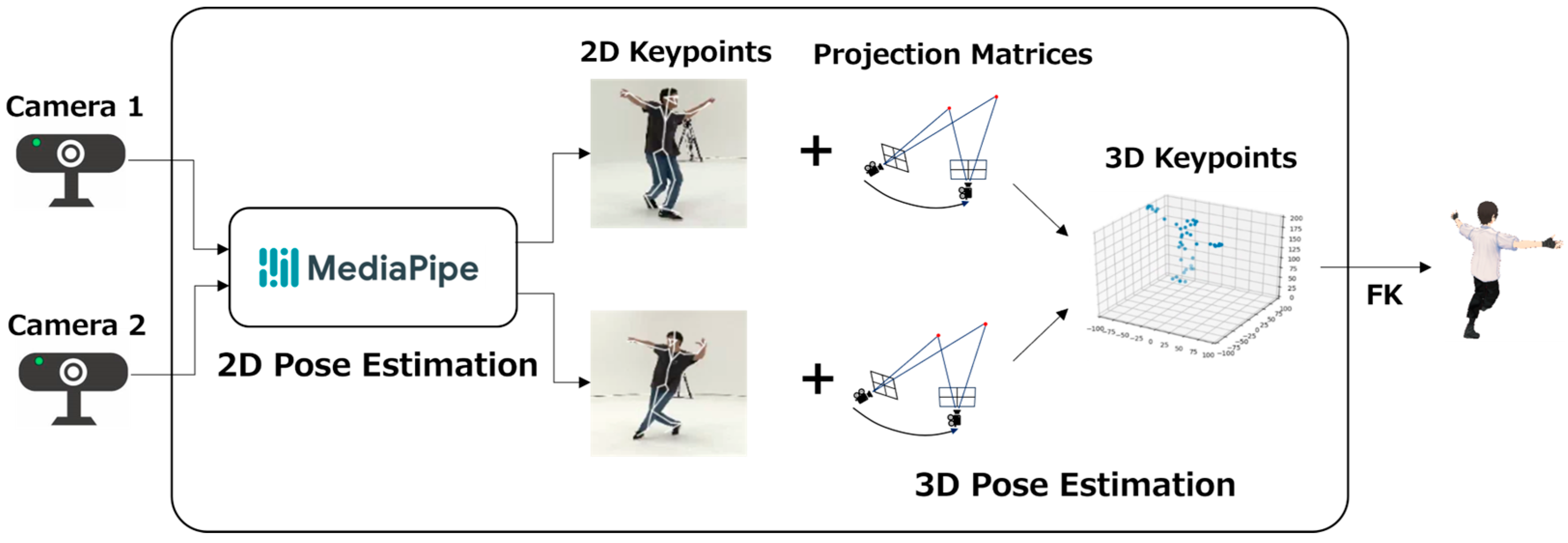
Figure 2.
Workflow of system.
Figure 2.
Workflow of system.
Figure 3.
Dance training system in use (real scene on the left; virtual space scene on the right).
Figure 3.
Dance training system in use (real scene on the left; virtual space scene on the right).
Figure 4.
Dance training scenes.
Figure 4.
Dance training scenes.
Figure 5.
Dance training system in use (evaluation scene on the left; reflection scene on the right).
Figure 5.
Dance training system in use (evaluation scene on the left; reflection scene on the right).
Figure 6.
Motion capture process.
Figure 6.
Motion capture process.
Figure 7.
MR-based camera setup.
Figure 7.
MR-based camera setup.
Figure 8.
Feedback example.
Figure 8.
Feedback example.
Figure 9.
Overview of our dance evaluation and feedback.
Figure 9.
Overview of our dance evaluation and feedback.
Figure 10.
Dance annotation system.
Figure 10.
Dance annotation system.
Figure 11.
Distribution of evaluation scores.
Figure 11.
Distribution of evaluation scores.
Figure 12.
Autoencoder model architecture.
Figure 12.
Autoencoder model architecture.
Figure 13.
Model architecture for contrastive learning.
Figure 13.
Model architecture for contrastive learning.
Figure 14.
Architecture of reference-guided model.
Figure 14.
Architecture of reference-guided model.
Figure 15.
Example of creating a correct label based on LDL.
Figure 15.
Example of creating a correct label based on LDL.
Figure 16.
Autoencoder learning curve.
Figure 16.
Autoencoder learning curve.
Figure 17.
Autoencoder visualization results (blue lines indicate the correct joint positions and orange lines indicate the results of visualizing the restored positions in a human body skeleton).
Figure 17.
Autoencoder visualization results (blue lines indicate the correct joint positions and orange lines indicate the results of visualizing the restored positions in a human body skeleton).
Figure 18.
Encoder learning curve with contrastive learning (Euclidean distance).
Figure 18.
Encoder learning curve with contrastive learning (Euclidean distance).
Figure 19.
Confusion matrices of evaluation model predictions (the three dancers in the test data, left, baseline; right, proposed method). The background color of each cell in the matrix is lighter for smaller values and darker for larger values.
Figure 19.
Confusion matrices of evaluation model predictions (the three dancers in the test data, left, baseline; right, proposed method). The background color of each cell in the matrix is lighter for smaller values and darker for larger values.
Figure 20.
Radar charts of evaluation model predictions (the three dancers in the test data). The blue line represents the correct score and orange the prediction score.
Figure 20.
Radar charts of evaluation model predictions (the three dancers in the test data). The blue line represents the correct score and orange the prediction score.
Figure 21.
Confusion matrices of evaluation model predictions (the last count in the test data, left, baseline; right, proposed method). The background color of each cell in the matrix is lighter for smaller values and darker for larger values.
Figure 21.
Confusion matrices of evaluation model predictions (the last count in the test data, left, baseline; right, proposed method). The background color of each cell in the matrix is lighter for smaller values and darker for larger values.
Figure 22.
Radar charts of evaluation model predictions (the last count in the test data).
Figure 22.
Radar charts of evaluation model predictions (the last count in the test data).
Table 1.
Comparison with previous studies. TAKAHASHI [
57]: Metrics obtained using a dual-camera setup. LEE (L) [
56]: Metrics obtained with a five-camera setup using linear calibration only. LEE (L + B) [
56]: Metrics obtained when bundle adjustment is additionally applied to LEE (L). OURS: Evaluation metrics obtained with our proposed dual-camera method.
| | | | | |
|---|
| Takahashi [57] | 0.368 | 5.355 | - | 2 |
| Lee (L) [56] | 0.043 | 1.414 | 1.817 | 5 |
| Lee (L + B) [56]: | 0.020 | 0.053 | 0.041 | 5 |
| Ours | 0.036 | 0.102 | 0.098 | 2 |
Table 2.
Professional advice.
Table 2.
Professional advice.
| Frequency Order | Advice Content |
|---|
| 1 | You are nervous and your body is not moving, so dance as hard as you can. |
| 2 | Dance a whole lot bigger. |
| 3 | Where you stop moving, stop tight. |
| 3 | Move your hands smoothly and with awareness of the flow of your hands. |
| 3 | Bend your knees and drop your center of gravity more. |
| 6 | Move your hands more clearly. |
| 6 | Go over your choreography again. |
Table 3.
Dance evaluation items.
Table 3.
Dance evaluation items.
| Evaluation Item | Evaluation Content |
|---|
| Dynamics | Elements of movement such as power, weight, and vigor |
| Sharpness | Continuity of movement, like precision and crispness |
| Scalability | Spatial aspects of movement, such as the magnitude and width of the dancer’s stride |
| Timing | Temporal features like rhythm and pace |
| Accuracy | Exactness of movements, including choreography, facial orientation, and rhythm |
| Stability | Aspects such as body control and balance, reflecting the steadiness and control of a dancer’s movements |
Table 4.
Content of dataset.
Table 4.
Content of dataset.
| Subjects | 1 coach
20 practitioners
7 elementary school students
6 junior high school students
5 high school students
2 university students |
| Number of dance data | 44 |
| Length of dance | 14.9 s |
| Number of videos | 176 |
| Number of annotations | 32 × 6 categories |
Table 5.
General criteria for kappa score.
Table 5.
General criteria for kappa score.
| Kappa Score | Interpretation |
|---|
| −1.0 | Perfect mismatch |
| 0.0 | Match by chance |
| 0.01–0.20 | Slight match |
| 0.21–0.40 | Generally match with |
| 0.41–0.60 | Moderate match |
| 0.61–0.80 | Fairly close match |
| 0.81–0.99 | Almost match |
| 1.0 | Perfect match |
Table 6.
Example of quadratic weighted kappa weights.
Table 6.
Example of quadratic weighted kappa weights.
| Weight | 1 | 2 | 3 | 4 | 5 |
|---|
| 1 | 1.0000 | 0.9375 | 0.7500 | 0.4375 | 0.0000 |
| 2 | 0.9375 | 1.0000 | 0.9375 | 0.7500 | 0.4375 |
| 3 | 0.7500 | 0.9375 | 1.0000 | 0.9375 | 0.7500 |
| 4 | 0.4375 | 0.7500 | 0.9375 | 1.0000 | 0.9375 |
| 5 | 0.0000 | 0.4375 | 0.7500 | 0.9375 | 1.0000 |
Table 7.
Autoencoder model parameters.
Table 7.
Autoencoder model parameters.
| Parameter | Search Range | Value |
|---|
| Number of GCN layers | 1–3 | 2 |
| Number of GCN filters | 16–512 | 128 |
| Bidirectional (encoder) | True, False | True |
| Bidirectional (decoder) | True, False | False |
| Number of LSTM units | 32–1024 | 512 |
| Number of units in dense layers | 32–1024 | 256 |
| Dropout rate | 0.0–0.5 | 0.1 |
| Learning rate | 0.00001–1 | 0.005 |
Table 8.
Evaluation model learning results (autoencoder).
Table 8.
Evaluation model learning results (autoencoder).
| | Dynamics | Sharpness | Scalability | Timing | Accuracy | Stability |
|---|
| LMA + RF | 0.575 | 0.548 | 0.450 | 0.562 | 0.585 | 0.539 |
| AE | 0.752 | 0.752 | 0.615 | 0.566 | 0.636 | 0.674 |
Table 9.
Parameters of encoder model with contrastive learning.
Table 9.
Parameters of encoder model with contrastive learning.
| Parameter | Search Range | Value |
|---|
| Number of LSTM layers | 1–3 | 2 |
| Bidirectional | True, False | True |
| Number of LSTM units | 32–1024 | 512 |
| Dropout rate | 0.0–0.5 | 0.4 |
| Representation vector size | 32–1024 | 64 |
| Embedding size | 32–1024 | 256 |
| Threshold | 0.0–6.0 | 2.0 |
| Learning rate | 0.00001–1 | 0.0005 |
| Batch size | 8–256 | 32 |
Table 10.
Learning results of encoder model with contrastive learning.
Table 10.
Learning results of encoder model with contrastive learning.
| Distance Calculation Method | Swap Error |
|---|
| Euclidean distance | 0.039 |
| Manhattan distance | 0.146 |
Table 11.
Parameters of evaluation model (reference-guided).
Table 11.
Parameters of evaluation model (reference-guided).
| Parameter | Search Range | Value |
|---|
| Vector combining method | Sub, Concat, Mul | Sub |
| Number of dense layers | 1–3 | 2 |
| Number of units in dense layers | 8–1024 | (256, 64) |
| Dropout rate | 0.0–0.5 | 0.2 |
| Learning rate | 0.00001–1 | 0.0005 |
| Batch size | 8–256 | 32 |
Table 12.
Evaluation model learning results (contrastive learning).
Table 12.
Evaluation model learning results (contrastive learning).
| | Dynamics | Sharpness | Scalability | Timing | Accuracy | Stability |
|---|
| LMA + RF | 0.575 | 0.548 | 0.450 | 0.562 | 0.585 | 0.539 |
| CL (Euclidean) | 0.785 | 0.762 | 0.666 | 0.747 | 0.759 | 0.797 |
| CL (Manhattan) | 0.658 | 0.635 | 0.593 | 0.660 | 0.571 | 0.700 |
Table 13.
Evaluation model learning results (dynamics).
Table 13.
Evaluation model learning results (dynamics).
| | Quadratic Weighted Kappa | Kappa | Correlation Coefficient | MAE |
|---|
| LMA + RF | 0.575 | 0.035 | 0.562 | 1.829 |
| CL | 0.785 | 0.117 | 0.793 | 1.238 |
| AE | 0.752 | 0.048 | 0.767 | 1.361 |
| CL + AE | 0.882 | 0.192 | 0.846 | 1.027 |
Table 14.
Evaluation model learning results (sharpness).
Table 14.
Evaluation model learning results (sharpness).
| | Quadratic Weighted Kappa | Kappa | Correlation Coefficient | MAE |
|---|
| LMA + RF | 0.546 | 0.003 | 0.585 | 1.895 |
| CL | 0.762 | 0.075 | 0.800 | 1.423 |
| AE | 0.752 | −0.003 | 0.805 | 1.402 |
| CL + AE | 0.890 | 0.185 | 0.846 | 1.032 |
Table 15.
Evaluation model learning results (scalability).
Table 15.
Evaluation model learning results (scalability).
| | Quadratic Weighted Kappa | Kappa | Correlation Coefficient | MAE |
|---|
| LMA + RF | 0.450 | 0.005 | 0.460 | 2.046 |
| CL | 0.666 | 0.060 | 0.675 | 1.578 |
| AE | 0.615 | 0.036 | 0.634 | 1.675 |
| CL + AE | 0.720 | 0.162 | 0.718 | 1.500 |
Table 16.
Evaluation model learning results (timing).
Table 16.
Evaluation model learning results (timing).
| | Quadratic Weighted Kappa | Kappa | Correlation Coefficient | MAE |
|---|
| LMA + RF | 0.562 | 0.152 | 0.523 | 1.862 |
| CL | 0.747 | 0.033 | 0.759 | 1.462 |
| AE | 0.566 | 0.102 | 0.614 | 1.617 |
| CL + AE | 0.775 | 0.058 | 0.778 | 1.310 |
Table 17.
Evaluation model learning results (accuracy).
Table 17.
Evaluation model learning results (accuracy).
| | Quadratic Weighted Kappa | Kappa | Correlation Coefficient | MAE |
|---|
| LMA + RF | 0.585 | 0.102 | 0.595 | 2.060 |
| CL | 0.759 | 0.038 | 0.854 | 1.505 |
| AE | 0.636 | 0.018 | 0.732 | 1.765 |
| CL + AE | 0.838 | 0.290 | 0.851 | 1.182 |
Table 18.
Evaluation model learning results (stability).
Table 18.
Evaluation model learning results (stability).
| | Quadratic Weighted Kappa | Kappa | Correlation Coefficient | MAE |
|---|
| LMA + RF | 0.539 | 0.170 | 0.581 | 1.461 |
| CL | 0.797 | 0.139 | 0.810 | 1.173 |
| AE | 0.674 | 0.100 | 0.625 | 1.415 |
| CL + AE | 0.886 | 0.436 | 0.881 | 0.735 |
Table 19.
Comparison with and without reference.
Table 19.
Comparison with and without reference.
| | Dynamics | Sharpness | Scalability | Timing | Accuracy | Stability |
|---|
| LMA + RF | 0.575 | 0.548 | 0.450 | 0.562 | 0.585 | 0.539 |
| No-reference | 0.858 | 0.791 | 0.837 | 0.838 | 0.756 | 0.825 |
| Reference-guided | 0.874 | 0.880 | 0.873 | 0.885 | 0.908 | 0.920 |
Table 20.
Degree of agreement on items requiring improvement.
Table 20.
Degree of agreement on items requiring improvement.
| | Accuracy | Precision | Recall | F1 Score |
|---|
| LMA + RF | 0.536 | 0.441 | 0.544 | 0.487 |
| CL + AE | 0.619 | 0.676 | 0.556 | 0.610 |
Table 21.
Lowest score accuracy.
Table 21.
Lowest score accuracy.
| | Accuracy |
|---|
| LMA + RF | 0.500 |
| CL + AE | 0.679 |


