Compensation Observer-Based Adaptive Output Feedback Control for Multi-Agent Systems

Abstract

This study presents a modified compensating observer control strategy for nonlinear multi-agent systems affected by unknown hysteresis signal loops. Compared to conventional high-gain observers, this approach introduces a novel compensation signal, effectively reducing the tracking error of traditional observers. Then, by utilizing a backstepping method, an adaptive output feedback controller is designed, such that the tracking error converges to the small neighborhood around the origin. Simulation experiments with and without the compensation term demonstrate that this control strategy can effectively reduce error, but it increases input chattering to some extent.

1. Introduction

The coordinated control of multi-agent systems has emerged as a pivotal area of contemporary research, driven by the proliferation of distributed network resources and the imperative for collaboration among various mechanical devices [1,2,3]. Key aspects of such systems encompass group interaction and communication, coordination and cooperation, and conflict resolution. A prominent example of these concepts is the multi-flight simulator system [4]. Additionally, multi-agent systems have notable applications in the healthcare sector [5].

Exploration of multi-agent systems has yielded numerous methodologies and control strategies aimed at ensuring consistent stability. For instance, dynamic surface control combined with a first-order low-pass filter has been utilized to address the inherent “differential explosion” issue in traditional recursive methods [6,7,8,9]. While this method simplifies computational complexity, it also introduces errors associated with filter computation and increases the number of control parameters, potentially compromising transient performance management. Recent research [10] has attempted to resolve the algebraic loop problem intrinsic to the backstepping method, thereby ensuring transient tracking performance, albeit at the cost of increased control complexity due to the introduction of new variables.

In addressing the problem of unknown states in high-order multi-agent systems, observers are often employed. Among these, the use of high-gain observers is a common research approach [11,12]. Through the application of such observers, disturbances within the system, including external input disturbances, system coupling, and other factors, can be effectively managed [13,14,15,16,17]. These mechanisms ensure the stability of the entire closed-loop system while optimizing the tracking performance of each subsystem. Various types of observers employ different methodologies; for example, interval observers utilize neural networks, resilient control techniques, and fuzzy equations to estimate unmeasurable states of the system [18]. By narrowing the interval width, this method ensures that the closed-loop system remains semi-globally ultimately bounded, allowing for a convergence of tracking and observation errors within a small neighborhood near the origin [19]. Similar developments have been documented in discrete systems [20]. Optimizations of high-gain observers involve dimensionality reduction, as seen in the current literature [21,22] where the observer model’s complexity is optimized within manageable limits while ensuring that all closed-loop signals are ultimately bounded under the influence of a continuously differentiable switching function. Therefore, building upon the research foundation of high-gain observers, this study considers the addition of compensatory terms to achieve error reduction and structural simplification.

Furthermore, with the expansion of material science applications, particularly in multi-agent systems equipped with intelligent materials, significant challenges arise. For example, piezoelectric ceramics and ionic polymer metal composites have gained attention due to their exceptional performance and desirable physical characteristics [23]. However, these materials also exhibit performance deficiencies, such as non-smoothness, nonlinearity, and hysteresis, which can significantly impact the precision and stability of control systems, particularly due to the effects of hysteresis signals and coupling characteristics [24]. To address nonlinear hysteresis inputs, two primary strategies are typically employed. The first strategy involves mitigating hysteresis effects through the development of an adaptive hysteresis inverse controller [25]. The second strategy, similar to the methods outlined in [26], employs an adaptive algorithm to reduce the impacts of hysteresis by modeling it with both linear and nonlinear components. Commonly referenced models include the dead zone hysteresis model, the Prandtl–Ishlinskii (PI) hysteresis model, and the Bouc–Wen hysteresis model. This study discusses the processing of hysteresis signals using the Prandtl–Ishlinskii model. The specific work content is as follows:

(1)

This study introduces a modified compensating observer scheme. By incorporating this compensatory mechanism, the proposed method effectively reduces tracking errors and confines them to a small region near zero while ensuring stability, compared to traditional control schemes.

(2)

Unlike most output feedback systems, the system investigated in this study involves unknown parameters, nonlinear coupling, and hysteresis interference, and the proposed compensating observer has more practical significance.

The proposed scheme in this study demonstrates superior performance in handling nonlinear multi-agent systems through numerical simulations and case studies while maintaining low computational complexity. This provides new insights and methods for controlling nonlinear multi-agent systems and lays a foundation for future research directions. By comparing with existing mainstream control strategies, this study not only highlights the advantages of the new method but also reveals its potential limitations in practical applications, thereby providing valuable references for further optimization and improvement.

The remainder of this paper is organized as follows. Section 2 outlines the relevant background information, problem models, assumptions, and lemmas necessary for understanding the subsequent analysis. In Section 3, we propose a decentralized adaptive output feedback backstepping approach that incorporates a high-gain observer. Section 4 provides a comprehensive stability analysis, which substantiates the stability and tracking capabilities of the system. Finally, Section 5 corroborates the effectiveness of our proposed design through simulation results based on an example presented earlier in the paper.

2. Establishing the Problem Model

2.1. Preliminaries

According to the principles of the graph theory presented in [10,11,12], the relationship among followers is represented here by a directed topological graph $G=\{U,T,M\}$, where $U=\{1,\cdots ,N\}$ denotes the set of nodes, $T=U\times U$ defines the set of edges, and $M=\left\{a_{ij}\right\}\in R^i$ is the adjacency matrix. If node $j$ can send data to node $i$, then $a_{ij}=1$ ; otherwise, $a_{ij}=0$. To facilitate system analysis, we employ the following lemmas and inequality theorems.

Lemma 1

[5]. The following formula is valid as long as there exist normal numbers $\Delta$, ${\sigma }_1$ , and ${\sigma }_2$ and a symmetrical positive definite matrix $P$ , where $E$ is the identity matrix. $D=\mathrm{diag}[\begin{array}{cccc}0& 1& \cdots & n_i-1\end{array}]$ :

$${\sigma }_{1}E\le DP+PD+2\Delta P\le {\sigma }_{2}E.$$

(1)

Lemma 2

[17]. There is a positive definite matrix $P$ that meets the following requirements if matrix $A_i-q_i{c}_i^T$ is a Hurwitz matrix:

$${\left(A_i-q_i{c}_i^T\right)}^{T}P+P\left(A_i-q_i{c}_i^T\right)=-E.$$

(2)

Lemma 3

[9]. The following inequality is met for any $d>0$ and $x\in R^i$ (where $R^i$ represents the set of real numbers):

$$0\le \left|x\right|-\frac{x^2}{\sqrt{x^2+d^2}}<d.$$

(3)

Theorem 1.

Young’s inequality:

$$\left\{\begin{array}{l}{\Theta }_i\Gamma e_{ij}\le \frac{\rho }{2}\theta \parallel \Gamma {\parallel }^2{e_{ij}}^2+\frac{1}{2\rho }\hfill \\ e_{ij}{ϵ}_{2j}\le \rho l_i^{1+2\Delta }{e_{ij}}^2+\frac{1}{4\rho }{l}_i{{\overbracket{ϵ}}_{2j}}^2\hfill \end{array}\right.$$

(4)

$$\left\{\begin{array}{l}\frac{\partial {\alpha }_{i-1}}{\partial y_i}{ϵ}_{2j}{e}_{ij}\le \rho l_i^{1+2\Delta }{\left(\frac{\partial {\alpha }_{i-1}}{\partial y_i}\right)}^2{e_{ij}}^2+\frac{1}{4\rho }{l}_i{{\overbracket{ϵ}}_{2j}}^2\hfill \\ \frac{\partial {\alpha }_{i-1}}{\partial y_i}{\Theta }_i\Gamma e_{ij}\le \frac{\rho }{2}{\left(\frac{\partial {\alpha }_{i-1}}{\partial y_i}\right)}^2\theta \parallel \Gamma {\parallel }^2{e_{ij}}^2+\frac{1}{2\rho }\hfill \end{array}\right..$$

(5)

The parameters that are already in place are known positive design parameters. The other parameters will be determined later.

2.2. Basic Model and Problem Hypothesis

We consider a set of nonlinear systems defined as follows. First, Equation (6) delineates the state equation:

$$\begin{array}{cc}\hfill {\dot{x}}_{ij}& =A_i{x}_{ij}+{\phi }_{0,i,j}\left(y_i\right)+{\displaystyle \sum _{k=1}^{r_i}{\phi }_{k,i,j}\left(y_i\right)}{a}_{k,i,j}+F_{i,j}\left(y_i\right)x_{ij}+b_i{H}_{i,j}(y_i)w_i\hfill \\ \hfill y_i& =c_i^T{x}_i\hfill \end{array}.$$

(6)

Let $x_{ij}={\left[\begin{array}{cccc}{x}_{i1}& x_{i2}& \cdots & x_{i{n}_i}\end{array}\right]}^T,x_{ij}\in R^i$ denote the $j$-th state variable of the $i$-th subsystem, where $j=1,2,\cdots ,n_i$ and $i=1,2,\cdots ,n$. The actual output of the $i$-th subsystem is $y_i\in R^i$. Here, the smooth nonlinear function vectors ${\phi }_{0,i,j}\left(y_i\right)\in R^i$ and ${\phi }_{k,i,j}\left(y_i\right)\in R^i$ are known, as is the lower triangular nonlinear function matrix $F_{i,j}\left(y_i\right)$. The matrix $H_{i,j}\left(y_i\right)$ is a known function matrix, while $a_{k,i,j}$ and $b_i$ are unknown, non-zero constant parameters. The structure of the matrix is as follows:

$$A_i=\left[\begin{array}{cc}0& E_{i-1}\\ 0& 0\end{array}\right]$$

(7)

$$c_i=\left[\begin{array}{ccc}\begin{array}{cc}1& 0\end{array}& \begin{array}{cc}0& 0\end{array}& \begin{array}{cc}\cdots & 0\end{array}\end{array}\right]=\left[\begin{array}{cc}1& 0_{\left(n_i-1\right)\times 1}\end{array}\right]$$

(8)

$$F_{i,j}\left(y_i\right)=\left[\begin{array}{ccc}\begin{array}{ccc}0& 0& 0\\ 0& f_{2,2}& 0\\ 0& f_{3,2}& f_{3,3}\end{array}& \cdots & \begin{array}{c}0\\ 0\\ 0\end{array}\\ ⋮& \ddots & ⋮\\ \begin{array}{ccc}0& f_{n,2}& f_{n,3}\end{array}& \cdots & f_{n,n_i}\end{array}\right]$$

(9)

$$H_{i,j}={\left[\begin{array}{cccc}{0}_{z-2,j}& \begin{array}{cc}0& H_{z,j}\end{array}& \cdots & H_{n,j}\end{array}\right]}^T$$

(10)

$${\phi }_{0,i,j}\left(y_i\right)={\left[\begin{array}{cccc}{\phi }_{0,1,j}\left(y_i\right)& {\phi }_{0,2,j}\left(y_i\right)& \cdots & {\phi }_{0,n,j}\left(y_i\right)\end{array}\right]}^T$$

(11)

$${\phi }_{k,i,j}\left(y_i\right)={\left[\begin{array}{cccc}{\phi }_{k,1,j}\left(y_i\right)& {\phi }_{k,2,j}\left(y_i\right)& \cdots & {\phi }_{k,n,j}\left(y_i\right)\end{array}\right]}^T$$

(12)

where $w_i$ is an input for hysteresis. The Prandtl–Ishlinskii model was selected as the hysteresis model in this study. The relevant formula and mathematical model are as follows:

$$w_i\left(t\right)={\sigma }_i{u}_i\left(t\right)+\mathcal{F}[u_i](t).$$

(13)

In the expression $\mathcal{F}[u_i](t)={\displaystyle {\int }_0^{R}k\left(r\right)}{\mathcal{F}}_r^{\Psi }[u_i](t)\mathit{dr}$, the function $k\left(r\right)$ is a continuous, non-negative known function, while ${\sigma }_i$ is an unknown, non-zero constant. This equation represents an area-based hysteresis model.

The design parameter $R$ serves as the upper limit of integration. In practical analysis, the influence of $k\left(r\right)$ can be neglected when $R$ approaches infinity ($R=\infty$). Consequently, both $k\left(r\right)$ and ${\mathcal{F}}_r^{\Psi }[u_i](t)\mathit{dr}$ are bounded, and $k\left(r\right)$ is determined by experimental data. As a result, the functions $\mathcal{F}[u_i](t)$ are also bounded. Thus, the range of $\mathcal{F}[u_i](t)$ is constrained to $\mathcal{F}$, or ${\mathcal{F}}_r^k[u_i](t)\mathit{dr}\le \mathcal{F}$.

This formulation describes the saturation play operator ${\mathcal{F}}_r^{\Psi }[u_i]$. The expression uses $u_i\left(t\right)$ and $w_i$, respectively, as the input and output of symmetrical hysteresis, which is constrained by the curve $\Psi$ and represented by a well-known, continuous, non-decreasing function. Here, $R$ indicates the hysteresis threshold:

$${\mathcal{F}}_r^{\Psi }[u_i](0){=f}_r^{\Psi }\left(u_i\left(0\right)\right)$$

(14)

$${\mathcal{F}}_r^{\Psi }[u_i]({t)=f}_r^{\Psi }\left(u_i\left(t\right),{\mathcal{F}}_r^{\Psi }[u_i](t_k)\right)$$

(15)

$$f_r^{\Psi }\left(u_i\left(t\right),w_i\right)=\max \left(\Psi \left(u_i\right)-r,\min \left(\Psi \left(u_i\right)+r,w_i\right)\right)$$

(16)

$$t_k<t<t_{k+1\hspace{1em}},0\le k\le M-1.$$

(17)

Next, we provide a monotone input signal, which is monotone in the interval $[t_k,t_{k+1}]$, and select the parameter number using the formula above, as follows:

$$\begin{gathered} {\sigma }_i=0.6,\Psi \left(u_i\right)=6\tanh \left(u_i\right),R=70,k\left(r\right)=0.9e^{-0.04{\left(r-0.5\right)}^2} \\ {u}_i=4\sin \left(10\pi t\right)+\cos \left(0.5\pi t\right) \end{gathered}$$

(18)

In this way, the hysteresis model diagram shown in Figure 1 can be obtained.

Figure 1. PI hysteresis input relation model diagram.

The hysteresis effect set in this study has an upper and lower limit, as shown in Figure 1. Here, we use the parameter $T$ to represent the range of the hysteresis effect, which is $T=H_{i,j}\left(y_i\right)\mathcal{F}[u_i](t)$. The parameter $H$ represents the last term of the hysteresis effect, and the parameter $h$ represents the minimum value of the hysteresis effect. Here, H = 20, h = −20.

Remark 1.

The hysteresis phenomenon represents one of the most prevalent nonlinear influences in real systems. However, the existing literature on hysteresis research, such as the research in [5,7,9,13,17,23], has not yet proposed efficient solutions. Therefore, this study continues to focus on hysteresis phenomena as the subject of analysis.

We suggest the following presumptions for the current system to simplify system analysis.

Proposition 1.

The output of the theory leader$y_r$ and its derivatives (${\dot{y}}_r$ and ${\ddot{y}}_r$ ) are known, bounded, and smooth functions. The simulation will provide this function’s information.

Proposition 2.

Let the parameter ${\lambda }_i$ in the equation of state be a normal integer that can satisfy the following expression to maintain generality using the Hurwitz Equation (14):

$${\chi }_i\left(s\right)={\lambda }_{i,m}{s}^m+\cdots +{\lambda }_{i,1}{s}^1+{\lambda }_{i,0}.$$

(19)

Remark 2

[27]. As the polynomial ${\chi }_i\left(s\right)={\lambda }_{i,m}{s}^m+\cdots +{\lambda }_{i,1}{s}^1+{\lambda }_{i,0}$ is a Hurwitz polynomial, the positivity of coefficients ensures that the real parts of the roots (zeroes) of the system are negative, thereby guaranteeing system stability.

Proposition 3.

The leader transmits at least one directed spanning tree to the follower in the directed graph $G$ composed of system (7).

Proposition 4.

If a smooth and integrable bounded positive function ${\sigma }_i\left(t\right)$ exists, the following expression (20) is fulfilled:

$$\underset{t\to +\infty }{\lim }{\displaystyle {\int }_0^t{\sigma }_i}\left({\rho }_i\right)d{\rho }_i\le {\sigma }_{\infty }\le +\infty .$$

(20)

3. Controller Design and Derivation

3.1. Design of the Gain Compensation Observer

We devised a number of compensation gain filters in the manner described below to estimate the unknown state of the nonlinear multi-agent system (7):

$$\begin{array}{c}{\dot{\epsilon }}_{0ij}=(A_i-l_i{L}_i{q}_i{c}_i^T){\epsilon }_{0ij}+F_{i,j}\left(y_i\right){\epsilon }_{0ij}+{\phi }_{0,i,j}\left(y_i\right)+l_i{L}_i{q}_i{y}_i\hfill \\ {\epsilon }_{0ij}=(A_i-l_i{L}_i{q}_i{c}_i^T){\epsilon }_{kij}+F_{i,j}\left(y_i\right){\epsilon }_{\mathrm{k}ij}+{\phi }_{\mathrm{k},i,j}\left(y_i\right)\hfill \\ {\dot{\epsilon }}_{sij}=(A_i-l_i{L}_i{q}_i{c}_i^T){\epsilon }_{sij}+F_{i,j}\left(y_i\right){\epsilon }_{sij}+H_{i,j}\left(y_i\right)u_i\left(t\right)\hfill \\ {\dot{\epsilon }}_{zij}=(A_i-l_i{L}_i{q}_i{c}_i^T){\epsilon }_{cij}+F_{i,j}\left(y_i\right){\epsilon }_{cij}+\frac{TH}{h^2+{\sigma }_{\infty }^2}\hfill \end{array}$$

(21)

The factors in this case have values of $i\in [\begin{array}{ccc}1& \cdots & n\end{array}],q_i={[\begin{array}{ccc}{q}_1& \cdots & q_n\end{array}]}^T\in R^i$, and $q_i$, which correspond to the observer’s design parameters. The dynamic gain of the filter is $l_i$, and its expression is ${\dot{l}}_i=-{\Lambda }_i{l}_i^2+{\Lambda }_i{l}_i{l}_0{\sigma }_2+l_i\zeta \left(y_i\right)$, while the dynamic gain at position ${\Lambda }_i$ denotes a favorable design feature. A function with slick positive elements is represented by $\zeta \left(y_i\right)$. A positive design parameter, represented by ${\sigma }_{\infty }$, will be explained subsequently. The gain begins with a number of $l_0$.

We estimate the status as

$${\widehat{x}}_{ij}={\epsilon }_{0ij}+{\displaystyle \sum _{i=1}^r{a}_{k,i,j}{\epsilon }_{kij}}+b_i{\sigma }_i{\epsilon }_{sij}+b_i{\epsilon }_{zij}.$$

(22)

The definition error is ${\dot{ϵ}}_{ij}=x_{ij}-{\widehat{x}}_{ij}$, and its derivative is expressed as

$${\dot{ϵ}}_{ij}=(A_i-l_i{L}_i{q}_i{c}_i^T){ϵ}_{ij}+F_{i,j}\left(y_i\right){ϵ}_{ij}+b_{i}T-b_i\frac{TH}{h^2+{\sigma }_{\infty }^2}.$$

(23)

Transformation of this error is achieved as follows:

$${\overline{ϵ}}_{ij}=l_i^{-\Delta }{L}_i^{-1}{ϵ}_{ij}.$$

(24)

We next define the Lyapunov equation as an expression of $V_{{\widehat{ϵ}}_{ij}}={\left({\overline{ϵ}}_{ij}\right)}^T{P}_i{\overline{ϵ}}_{ij}$ and $A_i-l_i{L}_i{q}_i{c}_i^T=l_i{L}_i\left(A_i-q_i{c}_i^T\right)L_i^{-1}$ and combine Formulas (14)–(18):

$$\begin{array}{ll}\hfill {\dot{V}}_{{\overline{ϵ}}_{ij}}& =-\frac{{\dot{l}}_i}{l_i}\left(2\Delta P+DP+PD\right){\overline{ϵ}}_{ij}^2-l_i{\overline{ϵ}}_{ij}^2+{\left({\overline{ϵ}}_{ij}\right)}^T\left(F^{T}P+PF\right){\overline{ϵ}}_{ij}\hfill \\ & +2l_i^{-\Delta }{L}_i^{-1}{\overline{ϵ}}_{ij}{b}_i\left(T-\frac{TH}{h^2+{\sigma }_{\infty }^2}\right)\hfill \end{array}.$$

(25)

Remark 3.

Compared to the methods described in [28,29], the quadratic form employed in this study not only exhibits fundamental quadratic characteristics but also offers a simpler form and more favorable mathematical properties. The convex nature of quadratic functions facilitates easier analysis and the derivation of system stability and convergence properties, as well as controller design.

Proposition 5.

There exists a smooth non-negative function $\zeta \left(y_i\right)$ that fulfills $\Vert F_i\left(y_i\right)\Vert \le \zeta \left(y_i\right)$. The dynamic gain is subjected to the flattening function whose word is $1.6y_i^2+0.1y_i+0.15$ according to us.

The compensation component and hysteresis effect can be reduced as follows by combining Lemma 1, Lemma 2, Proposition 5, and the aforementioned theorems:

$$T-\frac{TH}{h^2+{\sigma }_{\infty }^2}=\frac{T{h}^2+T{{\sigma }_{\infty }}^2-TH}{h^2+{{\sigma }_{\infty }}^2}=\frac{T\left(h^2-H\right)+T{{\sigma }_{\infty }}^2}{h^2+{{\sigma }_{\infty }}^2}\le H+\frac{H\left({{\sigma }_{\infty }}^2-H\right)}{h}$$

(26)

$$-\frac{{\dot{l}}_i}{l_i}\left(2\Delta P+DP+PD\right){\overline{ϵ}}_{ij}^2\le -{\sigma }_1\frac{{\dot{l}}_i}{l_i}\Vert {\overline{ϵ}}_{ij}{\Vert }^2$$

(27)

$$F^{T}P+PF\le 2\Vert \zeta \left(y_i\right)\Vert \Vert P\Vert .$$

(28)

Remark 4.

The primary purpose of introducing T is to compensate for the self-interference term in the traditional high-gain observer, thereby reducing the impact of interference terms and consequently decreasing observational errors.

On the other hand, $M=\left(H+\frac{H\left({{\sigma }_{\infty }}^2-H\right)}{h}\right)2l_i^{-\Delta }{L}_i^{-1}{\overline{ϵ}}_{ij}$, where $M$ represents a finite parameter. Finally, we can obtain the following:

$${\dot{V}}_{{\overline{ϵ}}_{ij}}\le -\left(\frac{{\dot{l}}_i}{l_i}{\sigma }_1+l_i-2\Vert P\Vert \Vert \zeta (y_i)\Vert \right){{\overline{ϵ}}_{ij}}^2+M.$$

(29)

Remark 5.

The value of M is very small due to the influence of observer compensation, dynamic gains, and related parameters, which are consistently greater than 1. This fact corresponds with the stability proof content, ensuring the validity of the stability analysis.

Remark 6.

The selection criterion for ${\sigma }_{\infty }$ is to ensure that the value of this expression is minimized, ideally approaching the value of $\sqrt{H}$. The purpose of this design is to ensure that the value of $M$ is sufficiently small, which will be further explained in the stability analysis section.

3.2. Controller Design

In this section, a controller is constructed by utilizing the adaptive backstepping method with a gain compensation observer. Subsystems are recursively designed.

Step 1: $i=1$

The tracking error is defined as $e_{1j}=y_1-y_r$. The origin of the phrase is

$${\dot{e}}_{1j}=x_{2j}+{\phi }_{0,1,j}\left(y_i\right)+{\displaystyle \sum _{k=1}^{r_i}{\phi }_{k,1,j}\left(y_i\right)}{a}_{k,1,j}+F_{1,j}\left(y_i\right)x_{1j}-{\dot{y}}_r.$$

(30)

The following changes were made:

$${\Theta }_i=\left[\begin{array}{lllllllll}{a}_{1,1,j}\hfill & a_{2,1,j}\hfill & \cdots \hfill & a_{r_1,1,j}\hfill & a_{1,2,j}\hfill & a_{2,2,j}\hfill & \cdots \hfill & a_{r_2,2,j}\hfill & b_i\hfill \end{array}\right]$$

(31)

$$\Gamma ={\left[\begin{array}{cccccccc}{\phi }_{1,1,j}\left(y_i\right)& {\phi }_{2,1,j}\left(y_i\right)& \cdots & {\phi }_{r_1,1,j}\left(y_i\right)& {\epsilon }_{12j}& {\epsilon }_{22j}& \cdots & \begin{array}{cc}{\epsilon }_{r_{2}2j}& {\epsilon }_{z2j}\end{array}\end{array}\right]}^T.$$

(32)

Substituting Equations (31) and (32) into (30) yields

$${\dot{e}}_{1j}={\epsilon }_{02j}+b_i{\sigma }_i{\epsilon }_{s2j}+{ϵ}_{2j}+{\phi }_{0,1,j}\left(y_i\right)+{\Theta }_i\Gamma +F_{1,j}\left(y_i\right)x_{1j}-{\dot{y}}_r$$

(33)

where ${\gamma }_{\theta }$ and ${\gamma }_p$ are positive design parameters. Then, we synchronously set $\theta =\max \left\{\Vert {\Theta }_i{\Vert }^2,\Vert {\sigma }_i{\Vert }^2\right\}$. Here, $\theta$ is an unknown parameter and $\rho$ is a positive design parameter.

Next, we apply Formula (34):

$${\epsilon }_{sij}=e_{ij}+{\mathit{\alpha }}_{i-1}.$$

(34)

At the same time, we set the auxiliary controller as

$${\mathit{\alpha }}_1=\widehat{p}{\overline{\mathit{\alpha }}}_1$$

(35)

$${\overline{\mathit{\alpha }}}_1=-c_{1j}{e}_{1j}-{\epsilon }_{02j}-{\phi }_{0,1,j}\left(y_i\right)+{\dot{y}}_r-\frac{\rho }{2}\widehat{\theta }\parallel \Gamma {\parallel }^2{e}_{1j}-\rho {l_i}^{1+2\Delta }{e}_{1j}$$

(36)

where $c_{1j}$ is the known normal number; $\widehat{\theta }$ is the estimated value; and $\tilde{\theta }=\theta -\widehat{\theta }$, $\widehat{\theta }$ is the estimated value of the unknown parameter $\theta$. Additionally, $\tilde{p}=p-\widehat{p}$, $\widehat{p}$ are estimates of unknown parameter $p$.

According to inequality Theorem 1, the two parameters are scaled as follows:

$$\left\{\begin{array}{l}{\Theta }_i\Gamma e_{1j}\le \frac{\rho }{2}\theta \parallel \Gamma {\parallel }^2{e_{1j}}^2+\frac{1}{2\rho }\hfill \\ e_{1j}{ϵ}_{2j}\le \rho l_i^{1+2\Delta }{e_{1j}}^2+\frac{1}{4\rho }{l}_i{{\overline{ϵ}}_{2j}}^2\hfill \end{array}\right..$$

(37)

The Lyapunov equation can be changed into the following shape by defining the new parameter ${\Xi }_1$. The expression of this function is defined below:

$${\dot{V}}_1\le -c_{1j}{e_{1j}}^2+\widehat{\theta }{e}_{1j}{e}_{2j}+\frac{1}{2\rho }+\frac{1}{4\rho }{l}_i{{\overline{ϵ}}_{2j}}^2-\frac{1}{{\gamma }_{\theta }}\tilde{\theta }\left(\dot{\widehat{\theta }}-{\Xi }_1\right)-\frac{b_i{\sigma }_i}{{\gamma }_p}\tilde{p}\left(\dot{\widehat{p}}+{\overline{\alpha }}_1{e}_{1j}\right)+{\dot{V}}_{{\overline{ϵ}}_{ij}}$$

(38)

Step 2: $i=2$

As above, we set the Lyapunov function under the condition of $i=2$ and obtain the following expression according to Formula (34):

$$\begin{array}{ll}\hfill {\dot{V}}_{2j}& ={\dot{V}}_{1j}+e_{2j}{\dot{e}}_{2j}\hfill \\ & ={\dot{V}}_{1j}+e_{2j}\left({\dot{\epsilon }}_{s2j}-{\dot{\mathit{\alpha }}}_1\right){\dot{V}}_{1j}+e_{2j}\left({\epsilon }_{s3j}-l_i{L}_i{q}_i{\epsilon }_{s1j}+F_{2,j}\left(y_i\right){\epsilon }_{s2j}-{\dot{\mathit{\alpha }}}_1\right)\hfill \end{array}.$$

(39)

One can then derive the following equation from the auxiliary controller:

$$\begin{array}{cc}\hfill {\dot{\mathit{\alpha }}}_1& =\frac{\partial {\alpha }_1}{\partial \widehat{\theta }}\dot{\widehat{\theta }}+\frac{\partial {\alpha }_1}{\partial \widehat{p}}\dot{\widehat{p}}+\frac{\partial {\alpha }_1}{\partial y_r}{\dot{y}}_r+\frac{\partial {\alpha }_1}{\partial {\dot{y}}_r}{\ddot{y}}_r+\frac{\partial {\alpha }_1}{\partial l_i}{\dot{l}}_i+\frac{\partial {\alpha }_1}{\partial {\phi }_{0,1,j}}{\dot{\phi }}_{0,1,j}+\frac{\partial {\alpha }_1}{\partial {\epsilon }_{02j}}{\dot{\epsilon }}_{02j}\hfill \\ & +\frac{\partial {\alpha }_1}{\partial {\epsilon }_{k2j}}{\dot{\epsilon }}_{k2j}+\frac{\partial {\alpha }_1}{\partial \Gamma }\Gamma +\frac{\partial {\alpha }_1}{\partial y}\left({\phi }_{0,1,j}\left(y_i\right)+{\epsilon }_{02j}+{ϵ}_{2j}+{\Theta }_i\Gamma \right)\hfill \end{array}$$

(40)

In addition, we define the expression of the following parameters:

$$\begin{array}{cc}\hfill {\mathcal{B}}_2& =-l_i{L}_i{q}_i{\epsilon }_{s1j}+F_{2,j}\left(y_i\right){\epsilon }_{s2j}-\frac{\partial {\alpha }_1}{\partial y_r}{\dot{y}}_r-\frac{\partial {\alpha }_1}{\partial {\dot{y}}_r}{\ddot{y}}_r-\frac{\partial {\alpha }_1}{\partial l_i}{\dot{l}}_i-\frac{\partial {\alpha }_1}{\partial {\phi }_{0,1,j}}{\dot{\phi }}_{0,1,j}\hfill \\ & -\frac{\partial {\alpha }_1}{\partial {\epsilon }_{02j}}{\dot{\epsilon }}_{02j}-\frac{\partial {\alpha }_1}{\partial \Gamma }\left({\dot{\epsilon }}_{k2j}+{\dot{\epsilon }}_{z2j}+{\dot{\phi }}_{k2j}\right)-\frac{\partial {\alpha }_1}{\partial y}\left({\phi }_{0,1,j}\left(y_i\right)+{\epsilon }_{02j}\right)-\frac{\partial {\alpha }_1}{\partial \widehat{p}}\dot{\widehat{p}}\hfill \end{array}$$

(41)

Then, we can obtain the following expression:

$${\dot{V}}_{2j}={\dot{V}}_{1j}+e_{2j}\left(e_{3j}+{\mathit{\alpha }}_2+{\mathcal{B}}_2-\frac{\partial {\alpha }_1}{\partial \widehat{\theta }}\dot{\widehat{\theta }}-\frac{\partial {\alpha }_1}{\partial y_i}\left({ϵ}_{2j}+{\Theta }_i\Gamma \right)\right).$$

At this time, we use inequality Theorem 1 again:

$$\left\{\begin{array}{l}\frac{\partial {\alpha }_1}{\partial y_i}{ϵ}_{2j}{e}_{2j}\le \rho l_i^{1+2\Delta }{\left(\frac{\partial {\alpha }_1}{\partial y_i}\right)}^2{e_{2j}}^2+\frac{1}{4\rho }{l}_i{{\overline{ϵ}}_{2j}}^2\hfill \\ \frac{\partial {\alpha }_1}{\partial y_i}{\Theta }_i\Gamma e_{2j}\le \frac{\rho }{2}{\left(\frac{\partial {\alpha }_1}{\partial y_i}\right)}^2\theta \parallel \Gamma {\parallel }^2{e_{2j}}^2+\frac{1}{2\rho }\hfill \end{array}\right..$$

(42)

This theorem is then substituted into the Lyapunov equation, and the following parameters are defined:

$$\left\{\begin{array}{l} {\Xi }_1={\gamma }_{\theta }\left(\frac{\rho }{2}\parallel \Gamma {\parallel }^2{e_{1j}}^2\right)\hfill \\ {\Xi }_2={\Xi }_1+{\gamma }_{\theta }\frac{\rho }{2}{\left(\frac{\partial {\alpha }_1}{\partial y_i}\right)}^2\parallel \Gamma {\parallel }^2{e_{2j}}^2+{\gamma }_{\theta }{e}_{1j}{e}_{2j}\hfill \end{array}\right..$$

(43)

The expression of the auxiliary controller can be obtained with Formula (44):

$$\begin{array}{ll}\hfill {\alpha }_2& =-c_{2j}{e}_{2j}-{\mathcal{B}}_2-\rho l_i^{1+2\Delta }{\left(\frac{\partial {\alpha }_1}{\partial y_i}\right)}^2{e}_{2j}-\widehat{\theta }{e}_{1j}-\frac{\rho }{2}{\left(\frac{\partial {\alpha }_1}{\partial y_i}\right)}^2\widehat{\theta }\parallel \Gamma {\parallel }^2{e}_{2j}\hfill \\ & +\frac{\partial {\alpha }_1}{\partial \widehat{\theta }}\left({\Xi }_2-{\gamma }_{\theta }{\gamma }_{\tilde{\theta }}\widehat{\theta }\right)\hfill \end{array}$$

(44)

where ${\gamma }_{\tilde{\theta }}$ is positive design parameter.

Substituting Formula (44) into (39), we can obtain the expression of the Lyapunov equation as

$$\begin{array}{cc}\hfill {\dot{V}}_{2j}& \le -c_{2j}{e}_{2j}^2-c_{1j}{e}_{1j}^2+e_{2j}{e}_{3j}+\frac{2}{2\rho }+\frac{2}{4\rho }{l}_i{\overline{ϵ}}_{2j}^2-\frac{1}{{\gamma }_{\theta }}\tilde{\theta }\left(\dot{\widehat{\theta }}-{\Xi }_2\right)\hfill \\ & -\frac{b_i{\sigma }_i}{{\gamma }_p}\tilde{p}\left(\dot{\widehat{p}}+{\overline{\alpha }}_1{e}_{1j}\right)-e_{2j}\frac{\partial {\alpha }_1}{\partial \widehat{\theta }}\left(\dot{\widehat{\theta }}-{\Xi }_2+{\gamma }_{\theta }{\gamma }_{\tilde{\theta }}\widehat{\theta }\right)+{\dot{V}}_{{\overline{ϵ}}_{ij}}\hfill \end{array}$$

(45)

Step 3: $i\in [3,z)$.

The following formula can be obtained using the same inversion calculation method:

$$\begin{array}{cc}\hfill {\mathit{\alpha }}_i& =-c_{ij}{e}_{ij}-e_{\left(i-1\right)j}-{\mathcal{B}}_i-\rho l_i^{1+2\Delta }{\left(\frac{\partial {\alpha }_{i-1}}{\partial y_i}\right)}^2{e}_{zj}-\frac{\rho }{2}{\left(\frac{\partial {\alpha }_{i-1}}{\partial y_i}\right)}^2\widehat{\theta }\parallel \Gamma {\parallel }^2{e_{ij}}^2\hfill \\ & +\frac{\partial {\alpha }_{i-1}}{\partial \widehat{\theta }}\left({\Xi }_i-{\gamma }_{\theta }{\gamma }_{\tilde{\theta }}\widehat{\theta }\right)+{\gamma }_{\theta }{\displaystyle \sum _{q=2}^{i-1}}{e}_q\frac{\partial {\alpha }_{q-1}}{\partial y_i}\left[\frac{\rho }{2}{\left(\frac{\partial {\alpha }_{i-1}}{\partial y_i}\right)}^2\parallel \Gamma {\parallel }^2{e}_{ij}\right]\hfill \end{array}$$

(46)

$${\Xi }_i={\Xi }_{i-1}+{\gamma }_{\theta }\frac{\rho }{2}{\left(\frac{\partial {\alpha }_1}{\partial y_i}\right)}^2\parallel \Gamma {\parallel }^2{e_{ij}}^2$$

(47)

$$\begin{array}{cc}\hfill {\dot{V}}_{ij}& \le -{\displaystyle \sum _{a=1}^i{c}_a^2}{e}_a^2+e_{\left(i-1\right)j}{e}_{ij}+\frac{i}{2\rho }+\frac{i}{4\rho }{l}_i{\overline{ϵ}}_{2j}^2-\frac{1}{{\gamma }_{\theta }}\tilde{\theta }\left(\dot{\widehat{\theta }}-{\Xi }_i\right)-\frac{b_i{\sigma }_i}{{\gamma }_p}\tilde{p}\left(\dot{\widehat{p}}+{\overline{\alpha }}_1{e}_{1j}\right)\hfill \\ & -{\displaystyle \sum _{b=2}^i{e}_{bj}\frac{\partial {\alpha }_{b-1}}{\partial \widehat{\theta }}\left(\dot{\widehat{\theta }}-{\Xi }_b+{\gamma }_{\theta }{\gamma }_{\tilde{\theta }}\widehat{\theta }\right)}+{\dot{V}}_{{\overline{ϵ}}_{ij}}\hfill \end{array}$$

(48)

Step 4: $i\in [z,n]$.

This section adds the $H_{i,j}$ function and hysteresis input environment. The input is defined as follows:

$$u_i(t)=\frac{1}{H_{i,j}\left(y_i\right)}\left({\alpha }_i-{\epsilon }_{s\left(i+1\right)j}\right).$$

(49)

The expression of ${\alpha }_i$ is the same as that in Formula (46). Next, we set the Lyapunov function to (50)

$$V_{ij}=\frac{1}{2}{e_{ij}}^2+V_{\left(i-1\right)j}.$$

(50)

The expression can be obtained by substituting the above parameters into the following calculation:

$$\begin{array}{cc}\hfill {\dot{V}}_{nj}& \le -{\displaystyle \sum _{i=1}^n{c}_i^2}{e}_i^2+\frac{n}{2\rho }+\frac{n}{4\rho }{l}_i{\overline{ϵ}}_{2j}^2-\frac{b_i{\sigma }_i}{{\gamma }_p}\tilde{p}\left(\dot{\widehat{p}}+{\overline{\alpha }}_1{e}_{1j}\right)-\frac{1}{{\gamma }_{\theta }}\tilde{\theta }\left(\dot{\widehat{\theta }}-{\Xi }_n\right)\hfill \\ & -{\displaystyle \sum _{i=2}^n{e}_{ij}\frac{\partial {\alpha }_i}{\partial \widehat{\theta }}\left(\dot{\widehat{\theta }}-{\Xi }_n+{\gamma }_{\theta }{\gamma }_{\tilde{\theta }}\widehat{\theta }\right)}+{\dot{V}}_{{\overline{ϵ}}_{ij}}\hfill \end{array}$$

(51)

Let the parameter value be

$$\begin{array}{l}\dot{\widehat{\theta }}={\Xi }_n-{\gamma }_{\theta }{\gamma }_{\tilde{\theta }}\widehat{\theta }\\ \dot{\widehat{p}}=-{\overline{\alpha }}_1{e}_{1j}\end{array}.$$

(52)

In combination with Equation (51), the final expression of the Lyapunov equation can be obtained as follows:

$${\dot{V}}_{nj}\le -{\displaystyle \sum _{i=1}^n{c}_i^2}{e}_i^2+\frac{n}{2\rho }+\frac{n}{4\rho }{l}_i{{\overline{ϵ}}_{2j}}^2+{\gamma }_{\tilde{\theta }}\tilde{\theta }\widehat{\theta }-\left(\frac{{\dot{l}}_i}{l_i}{\sigma }_1+l_i-2\Vert P\Vert \Vert \zeta (y_i)\Vert \right){{\overline{ϵ}}_{ij}}^2+M.$$

(53)

4. Stability Analysis

This section is dedicated to analyzing the stability and tracking performance of the proposed control scheme. The globally stable operation and precise tracking capabilities of the closed-loop, decentralized, adaptive control system are ensured by incorporating a specially designed high-gain compensation observer.

Remark 7.

Consider a closed-loop system composed of the controlled system (7), the hysteresis signal (11), the compensation filter (14), the update law (24), and Equations (31) and (33). Next, select appropriate values for the gain’s positive design parameters $c_i$, ${\gamma }_{\tilde{\theta }}$, ${\Lambda }_i$, $l_0$, and $\zeta \left(y_i\right)$. The tracking error of each subsystem within the closed-loop decentralized control system converges to an arbitrarily small residual set, while all signals remain globally uniformly bounded.

Remark 8.

Notably, the proposed approach can effectively handle a wider range of interference signals, and system (7) encompasses more interference factors than systems in the existing literature. Thus, this system represents a broader category of multi-agent systems. The following are the key certification elements.

To summarize, let the Lyapunov function of the whole be $V_{nj}=V_{\left(n-1\right)j}+\frac{1}{2}{e}_{nj}^2$, where the value is $\left[2,\cdots ,n\right]$.

Next, use Young’s inequality, inequality Theorem 1, to extend and reduce Formula (55), as shown below:

$${\gamma }_{\tilde{\theta }}\tilde{\theta }\widehat{\theta }\le \frac{{\gamma }_{\tilde{\theta }}}{2}{\theta }^2-\frac{{\gamma }_{\tilde{\theta }}}{2}{\tilde{\theta }}^2.$$

(54)

Because of the universal existence of $\frac{n}{4\rho }{l}_i{{\overline{ϵ}}_{2j}}^2\le \frac{n}{4\rho }{l}_i\Vert {\overline{ϵ}}_{ij}{\Vert }^2$, parameter $\rho =n$ and the following equations are designed:

$$LR=\frac{{\dot{l}}_i}{l_i}{\sigma }_1+l_i-\frac{1}{4}{l}_i-2\Vert P\Vert \Vert \zeta (y_i)\Vert$$

(55)

$$\stackrel{°}{M}=M+\frac{1}{2}+\frac{{\gamma }_{\tilde{\theta }}}{2}{\theta }^2.$$

(56)

Combining (55)–(58), we can obtain Formula (59):

$${\dot{V}}_{nj}\le -{\displaystyle \sum _{i=1}^n{c}_i^2}{e}_i^2-\frac{{\gamma }_{\tilde{\theta }}}{2}{\tilde{\theta }}^2-\left(LR\right){{\overline{ϵ}}_{ij}}^2+\stackrel{°}{M}.$$

(57)

Then, set the parameters in dynamic gain ${\dot{l}}_i=-{\Lambda }_i{l}_i^2+{\Lambda }_i{l}_i{l}_0{\sigma }_2+l_i\zeta \left(y_i\right)$ as follows:

$${\sigma }_1=2\Vert P\Vert ,{\sigma }_2={\sigma }_1+0.2,{\Lambda }_i=\frac{1}{2{\sigma }_2},l_0=1$$

(58)

where $\Vert P\Vert$ is set to 0.5 in the simulation. The following outcomes can be obtained using this setting technique, which effectively reduces the interference of parameter variables:

$$LR=\left(\frac{3}{4}-\frac{{\sigma }_1}{2\left({\sigma }_1+0.2\right)}\right)l_i+\Vert P\Vert \Vert l_0\Vert .$$

(59)

For Formula (59), we selected the design parameters to meet the standard requirements:

$$\begin{gathered} c_i\ge \Omega \\ {\gamma }_{\tilde{\theta }}\ge \frac{2\Omega }{{\gamma }_{\theta }} \\ LR\ge \Omega \end{gathered}$$

(60)

where $\Omega$ is the positive term parameter designed in this study. Combining this formula with Formula (59), we can obtain

$${\dot{V}}_{nj}\le -2\Omega V_{nj}+\stackrel{°}{M}.$$

(61)

Next, solve the integral inequality:

$$0\le V_{nj}\left(t\right)\le \frac{\stackrel{°}{M}}{2\Omega }+\left(V_{nj}\left(0\right)-\frac{\stackrel{°}{M}}{2\Omega }\right)e^{-2\Omega T}.$$

(62)

In addition, when $t\to \infty$, the limit value can be obtained:

$$\underset{t\to \infty }{\lim }{V}_{nj}\left(t\right)=\frac{\stackrel{°}{M}}{2\Omega }.$$

(63)

Here, the parameters ${ϵ}_{ij}$, $e_{ij}$, $\tilde{\theta }$, and $\tilde{p}$ are bounded. Through the design process of Formulas (22)–(34), we can obtain expressions of the following main variables:

$$\begin{array}{l}{\dot{ϵ}}_{ij}=x_{ij}-{\widehat{x}}_{ij}\\ e_{1j}=y_1-y_r\\ e_{2j}={\epsilon }_{s2j}-{\mathit{\alpha }}_1\\ ⋮\\ e_{ij}={\epsilon }_{sij}-{\mathit{\alpha }}_{i-1}\end{array}.$$

(64)

The adjusted observer parameter ${\overline{ϵ}}_{ij}$ is also bounded, as both the expected value $y_r$ and dynamic gain $l_i$ are bounded according to our theoretical framework. Once the parameters of the compensatory observer, such as ${\epsilon }_{0ij}$, ${\epsilon }_{kij}$, ${\epsilon }_{sij}$, and ${\epsilon }_{zij}$, are confirmed to be finite, it can be demonstrated that the state variable $x_{ij}$ and the auxiliary controller ${\mathit{\alpha }}_i$ are also bounded. As a result, the integral discrepancy shown in Equation (62) can be resolved as follows:

$$\underset{t\to \infty }{\lim }\left|e_{1j}\right|=\underset{t\to \infty }{\lim }\sqrt{2V_{nj}\left(t\right)}=\sqrt{\frac{\stackrel{°}{M}}{\Omega }}.$$

(65)

Ultimately, variables $\stackrel{°}{M}$ and $\Omega$ are unrelated to one another. Through properly increasing $c_i$ , ${\gamma }_{\tilde{\theta }}$ , ${\gamma }_{\theta }$ , $LR$ , and $l_0$ , the larger value of $\Omega$ in Formula (59) can be selected. This step provides all remaining evidence.

Remark 9.

The compensation-based control strategy effectively reduces errors by lowering the key system parameters $\stackrel{°}{M}$. With appropriately chosen design parameters, the system errors can be reduced to zero under specific conditions.

5. Simulation Examples and a System Analysis of Control Strategies

This section presents two cases to illustrate the feasibility of our design strategy using numerical examples and gear system models. The objective of this control strategy is to progressively align each subsystem’s actual output $y_i$ with its desired output $y_r$ by utilizing an adaptive control law $u_i\left(t\right)$, developed through a compensatory observer control scheme. In this context, the differential equation ${\ddot{y}}_r+2{\dot{y}}_r+y_r=\sin t$ defines the optimal output $y_r$.

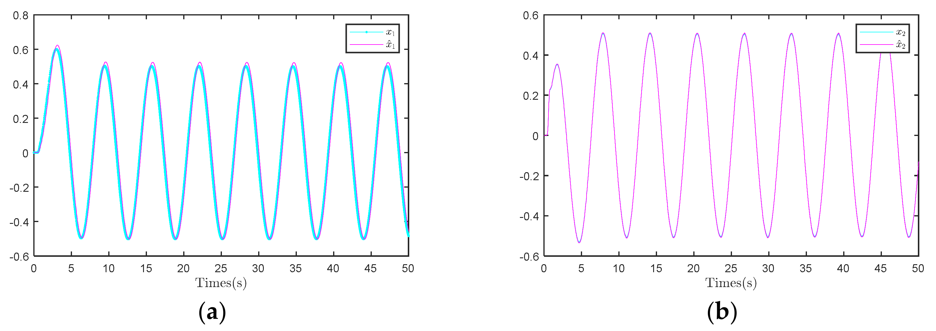
5.1. Numerical Example

We consider the following second-order numerical system:

$$\begin{array}{l}\left\{\begin{array}{l}{\dot{x}}_{11}\begin{array}{cc}=x_{12}& \end{array}\hfill \\ {\dot{x}}_{12}=0.2\sin \left(2y_1\right)+f_{1,2}{x}_2+b_1{H}_{12}{w}_1\hfill \end{array}\right.\\ y_1=x_{11}\end{array}$$

(66)

where $f_{1,2}=-2,b_1=1,H_{12}=0.1$. The remaining parameters are all set to zero.

To validate the effectiveness of the control strategy, we set the initial state of the control system to zero and compare the simulation results between the compensation observer control scheme and the traditional observer control scheme.

The compensatory observer control scheme proposed in this design introduces a compensation term $\frac{TH}{h^2+{{\sigma }_{\infty }}^2}$ into the traditional observer. Consequently, the traditional observer control scheme follows the observer structure shown in Equation (67), but without the compensation term. To ensure a fair comparison, all other parameters remain identical:

$$\begin{array}{c}{\dot{\epsilon }}_{0ij}=(A_i-l_i{L}_i{q}_i{c_i}^T){\epsilon }_{0ij}+F_{i,j}\left(y_i\right){\epsilon }_{0ij}+{\phi }_{0,i,j}\left(y_i\right)+l_i{L}_i{q}_i{y}_i\hfill \\ {\dot{\epsilon }}_{kij}=(A_i-l_i{L}_i{q}_i{c_i}^T){\epsilon }_{kij}+F_{i,j}\left(y_i\right){\epsilon }_{kij}+{\phi }_{k,i,j}\left(y_i\right)\hfill \\ {\dot{\epsilon }}_{sij}=(A_i-l_i{L}_i{q}_i{c_i}^T){\epsilon }_{sij}+F_{i,j}\left(y_i\right){\epsilon }_{sij}+H_{i,j}\left(y_i\right)u_i\left(t\right)\hfill \\ {\dot{\epsilon }}_{zij}=(A_i-l_i{L}_i{q}_i{c_i}^T){\epsilon }_{cij}+F_{i,j}\left(y_i\right){\epsilon }_{cij}\hfill \end{array}$$

(67)

Figure 2 presents the compensation observer control strategy, while Figure 3 illustrates the traditional controller control strategy. The error range in Figure 2b is smaller, indicating better tracking performance. This result further validates the superiority of the compensation observer control strategy.

Figure 2. Results under the compensation control strategy. (a) Trajectory tracking diagram of System 1. (b) System 1 output error.

Figure 3. Results under the traditional control strategy. (a) Trajectory tracking diagram of System 1. (b) System 1 output error.

Comparing the input waveforms between Figure 4 and Figure 5 indicates that under both control strategies, the input waveform of the overall system exhibits periodic variations. However, under the compensation strategy, the system input presents localized oscillations. This result represents a drawback of the control scheme, indicating a limitation in its ability to mitigate localized oscillations in the system input.

Figure 4. Input to System 1 under the compensation control strategy.

Figure 5. Input to System 1 under the traditional control strategy.

The dynamic behavior depicted in Figure 6, showing periodic states of the system output in three-dimensional state space, indicates the stable periodic responses of the system to certain inputs or initial conditions, indirectly suggesting a degree of stability in the system.

Figure 6. State space tracking performance of System 1.

As shown in Figure 7a, the derivative of the dynamic gain exhibits periodic oscillations. This phenomenon is similar to observations in Figure 7b. Additionally, the waveforms of ${\dot{\widehat{\theta }}}_i$ and $\dot{\widehat{p}}$ trend towards zero, indicating that the integrated values of these parameters are bounded. This characteristic may reflect the stability of the system dynamics, as the integrated values of the parameters are constrained, leading to limited variations in the system state within a finite range.

Figure 7. Results under the compensation control strategy. (a) Derivation of three parameters of System 1. (b) Waveform diagram of parameter $l_i$. (c) Waveform diagram of parameter ${\dot{\widehat{\theta }}}_i$. (d) Waveform diagram of parameter $\dot{\widehat{p}}$.

Based on the results shown in Figure 8, the waveforms of $x_i$ and ${\widehat{x}}_i$ are nearly identical, indicating that the observer can accurately track and predict the system’s state variables. This result demonstrates that the observer effectively estimates the system state in dynamic environments, thereby providing a necessary foundation for the performance of the stringent controller.

Figure 8. Comparison of observer performance. (a) $x_1$ and ${\widehat{x}}_1$ in System 1; (b) $x_2$ and ${\widehat{x}}_2$ in System 1.

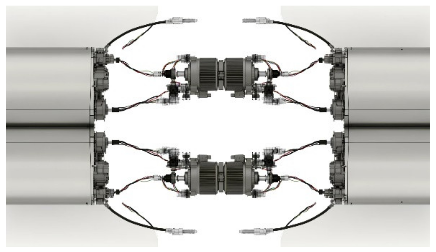
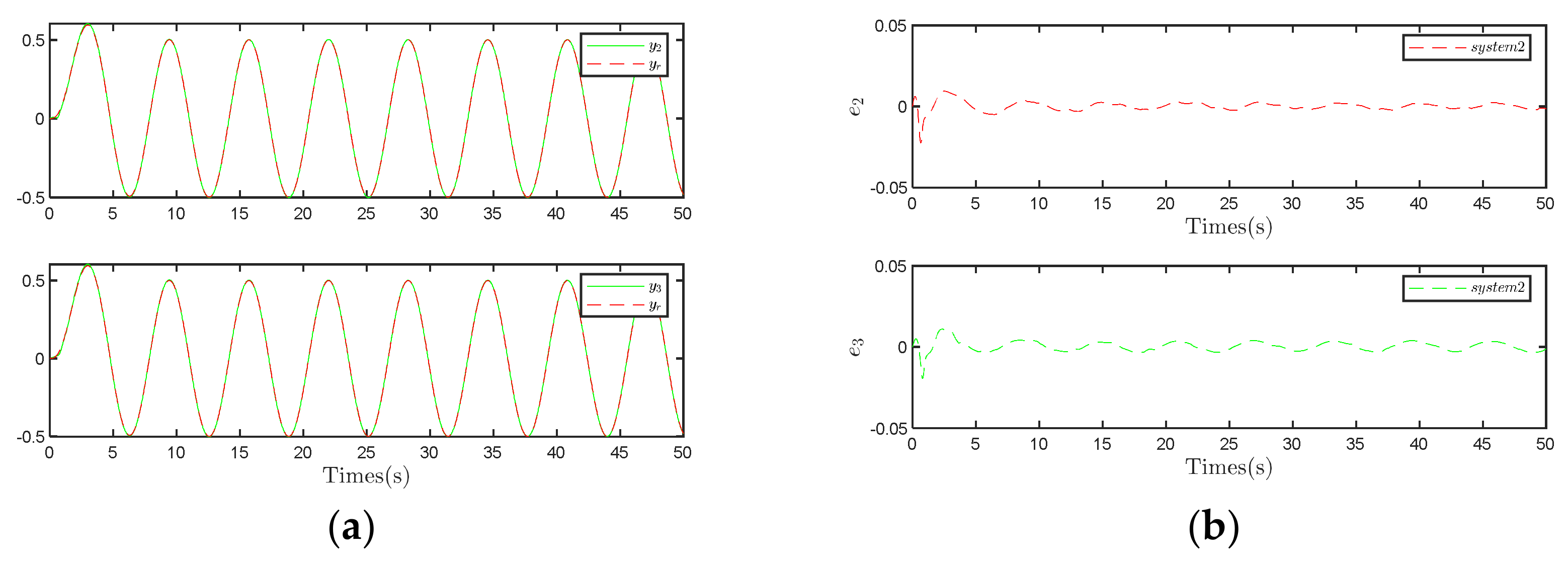
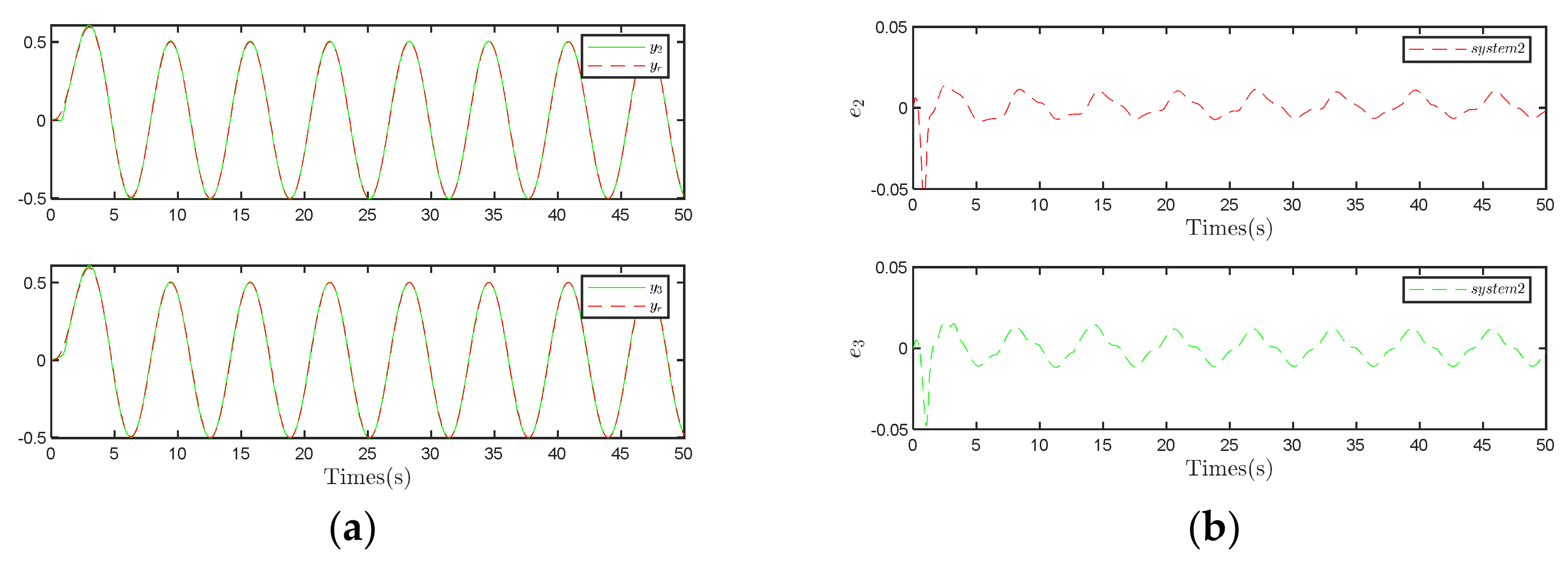
5.2. Pratical Example

In this section, we employ a dual-motor coupled control system as an example of the simulation. The instance model of this control system is illustrated in Figure 9. Here, we treat the two motors as independent agents within a multi-agent system. Each agent is independently controlled, and overall stability is achieved by coordinating the two agents via controllers or information transmission.

Figure 9. A dual-motor coupled control system.

The physical meanings of the parameters are as follows: ${\theta }_2$ is the drive rotation angle, and ${\theta }_3$ is the load rotation angle, which are represented by $x_{21}$ and $x_{31}$, respectively. $J_1$ is the moment of inertia of the load, $J_d$ is the moment of inertia of the driver, $g_r$ is the gear tooth ratio, $k_1$ is the damping of the driver, $k_2$ is the load damping, and $k$ is the torsional elastic constant.

The state equation of the system is

$$\begin{array}{l}\left\{\begin{array}{l}{\dot{x}}_{21}\begin{array}{c}=x_{22}+{\phi }_{0,2,1}\end{array}\hfill \\ {\dot{x}}_{22}={\phi }_{0,2,2}+f_{2,2}{x}_2+a_{k,2,2}{\phi }_{k,2,2}+b_2{H}_{2,2}{w}_2\hfill \end{array}\right.\\ y_2=x_{22}\end{array}$$

(68)

$$\begin{array}{l}\left\{\begin{array}{l}{\dot{x}}_{31}\begin{array}{c}=x_{32}+{\phi }_{0,3,1}\end{array}\hfill \\ {\dot{x}}_{32}={\phi }_{0,3,2}+f_{3,2}{x}_2+a_{k,3,2}{\phi }_{k,3,2}+b_3{H}_{3,2}{w}_3\hfill \end{array}\right.\\ y_3=x_{32}\end{array}.$$

(69)

In Formula (68) of subsystem 2,

$$\begin{array}{c}{f}_{2,2}=-\frac{k_1}{J_d},b_2=1,H_{22}=0.1,a_{k,2,2}=1\hfill \\ {\phi }_{0,2,1}=0.05\cos \left(3y_2\right)-0.02\sin (y_2-0.5)\hfill \\ {\phi }_{0,2,2}=0.5\sin \left(2y_2-0.5\right),{\phi }_{k,2,2}=\frac{kA}{J_d}\left(A{y}_2-y_3\right).\hfill \end{array}$$

(70)

In Formula (69) in subsystem 3,

$$\begin{array}{c}{f}_{3,2}=-\frac{k_1}{J_d},b_3=1,H_{32}=0.1,a_{k,3,2}=1\hfill \\ {\phi }_{0,3,1}=0.02\cos \left(y_3\right)-0.02\sin (y_3-0.5)\hfill \\ {\phi }_{0,3,2}=0.5\tan \left(2y_3\right),{\phi }_{k,3,2}=\frac{k}{J_1}\left(A{y}_2-B{y}_3\right)\hfill \end{array}.$$

(71)

Next, we set the parameter values as follows:

$$\begin{array}{c}A=\frac{1}{gr},k=1,k_1=0.8,k_2=0.6,J_1=1.2,\hfill \\ J_d=1,gr=0.8,B=1,\Delta =1,{\gamma }_{\tilde{\theta }}=2,{\gamma }_{\theta }=4\hfill \\ c_1=c_2=20,q_1=2,q_2=1,\rho =2,.\hfill \end{array}$$

To summarize, the simulation operation effect of the system can be obtained as follows:

Comparing Figure 10 with Figure 11 yields a consistent conclusion, indicating that employing the compensation observer control strategy can further reduce tracking errors. This finding underscores the efficacy of the compensation observer control strategy in enhancing the system’s tracking performance.

Figure 10. Results under the compensation control strategy. (a) Trajectory tracking diagram of System 2 and 3. (b) System 2 and 3 output error.

Figure 11. Results under the traditional control strategy. (a) Trajectory tracking diagram of System 2 and 3. (b) System 2 and 3 output error.

A comparative analysis of Figure 12 and Figure 13 similarly reveals an inherent flaw in the compensation observer control strategy: the exacerbation of input oscillations. This observation highlights a limitation of the compensational observer control strategy, indicating its tendency to amplify input oscillations. However, the degree of oscillation amplification is relatively mild and remains within an acceptable range.

Figure 12. Input to System 2 and 3 under the compensation control strategy.

Figure 13. Input to System 2 and 3 under the traditional control strategy.

Figure 14 graphically depicts the trajectories of Systems 2 and 3 within the state space, indicating a nearly complete overlap between them. This significant overlap not only underscores the high effectiveness of the control strategy in tracking the desired trajectory but also confirms the existence of a stable periodic response in both systems. The results from the comparative experiments further support these findings.

Figure 14. State space tracking performance of system 2 and 3.

Figure 15 presents the actual and estimated values of the first state variable. Here, the overlap between $x_{21}$  and ${\widehat{x}}_{21}$, as well as that between $x_{31}$  and ${\widehat{x}}_{31}$, indicates that the observer can closely match the true state of the system. The superior fitting accuracy of the second state variable can be observed in Figure 16, as indicated by the minimal deviation between $x_{22}$  and ${\widehat{x}}_{22}$, as well as $x_{32}$  and ${\widehat{x}}_{32}$. This level of precision in estimating the second state variable highlights the enhanced performance of the observer in multi-dimensional settings, which is crucial to effectively control multi-agent systems.

Figure 15. The comparison of observer performance.

Figure 16. The comparison of observer performance.

6. Conclusions and Further Research

This study introduced a modified compensatory observation scheme that markedly differs from traditional observation methods and was specifically designed for a class of nonlinear multi-agent systems influenced by an unknown hysteresis signal loop. This innovative approach not only significantly reduces tracking errors but also substantially enhances overall system tracking performance. However, we observed that under certain conditions, the compensatory observer control strategy may inadvertently increase input oscillations. Although these oscillations are relatively mild, it is essential to consider their potential impacts on overall system control and stability.

Future research will focus on further optimizing the system’s design. This includes detailed studies on parameter adjustments, structural enhancements, sensor layout optimization, and other aspects. These efforts aim to refine the compensatory observation scheme, minimize any adverse effects, and improve the robustness and reliability of the control strategy. Ultimately, such advancements will contribute to significant technological progress and development in related fields.

References

- Montagna, S.; Castro Silva, D.; Henriques Abreu, P.; Ito, M.; Schumacher, M.I.; Vargiu, E. Autonomous Agents and Multi-Agent Systems Applied in Healthcare. Artif. Intell. Med. 2019, 96, 142–144. [Google Scholar] [CrossRef] [PubMed]
- Cong, Z. Distributed ESO Based Cooperative Tracking Control for High-Order Nonlinear Multiagent Systems with Lumped Disturbance and Application in Multi Flight Simulators Systems. ISA Trans. 2018, 74, 217–228. [Google Scholar] [CrossRef] [PubMed]
- Wang, L.; Chen, M.Z.Q.; Gao, Z.; Wu, C.W.; Lin, Z. Special Issue on “Distributed Coordination Control for Multi-Agent Systems in Engineering Applications”. ISA Trans. 2017, 71, 1–2. [Google Scholar] [CrossRef] [PubMed]
- De Wilde, P.; Briscoe, G. Stability of Evolving Multiagent Systems. IEEE Trans. Syst. Man Cybern. Part B (Cybern.) 2011, 41, 1149–1157. [Google Scholar] [CrossRef] [PubMed]
- Liu, Y.; Fang, Z.; Li, Y. Global Decentralized Output Feedback Control for Interconnected Time Delay Systems with Saturated PI Hysteresis. J. Frankl. Inst. 2020, 357, 5460–5484. [Google Scholar] [CrossRef]
- Nguyen, T.T.; Nguyen, N.D.; Nahavandi, S. Deep Reinforcement Learning for Multiagent Systems: A Review of Challenges, Solutions, and Applications. IEEE Trans. Cybern. 2020, 50, 3826–3839. [Google Scholar] [CrossRef] [PubMed]
- Cui, G.; Xu, S.; Ma, Q.; Li, Y.; Zhang, Z. Prescribed Performance Distributed Consensus Control for Nonlinear Multi-Agent Systems with Unknown Dead-Zone Input. Int. J. Control 2017, 91, 1053–1065. [Google Scholar] [CrossRef]
- Gong, A.; Xie, X.; Yue, D.; Xia, J. Multi-instant observer design of discrete-time fuzzy systems via an enhanced gain-scheduling mechanism. IEEE Trans. Cybern. 2022, 53, 2876–2885. [Google Scholar] [CrossRef] [PubMed]
- Hua, C.; Liu, S.; Li, Y.; Guan, X. Distributed adaptive output feedback leader-following consensus control for nonlinear multiagent systems. IEEE Trans. Syst. Man Cybern. Syst. 2018, 50, 4309–4317. [Google Scholar] [CrossRef]
- Huang, D.; Yang, C.; Pan, Y.; Cheng, L. Composite learning enhanced neural control for robot manipulator with output error constraints. IEEE Trans. Ind. Inform. 2019, 17, 209–218. [Google Scholar] [CrossRef]
- Li, W.; Zhang, Z.; Ge, S.S. Dynamic Gain Reduced-Order Observer-Based Global Adaptive Neural-Network Tracking Control for Nonlinear Time-Delay Systems. IEEE Trans. Cybern. 2022, 53, 7105–7114. [Google Scholar] [CrossRef] [PubMed]
- Li, Z.; Liu, J.; Huang, Z.; Peng, Y.; Pu, H.; Ding, L. Adaptive impedance control of human–robot cooperation using reinforcement learning. IEEE Trans. Ind. Electron. 2017, 64, 8013–8022. [Google Scholar] [CrossRef]
- Liu, G.; Zhao, L.; Yu, J. Adaptive finite-time consensus tracking for nonstrict feedback nonlinear multi-agent systems with unknown control directions. IEEE Access 2019, 7, 155262–155269. [Google Scholar] [CrossRef]
- Liu, Y.H. Adaptive dynamic surface asymptotic tracking for a class of uncertain nonlinear systems. Int. J. Robust Nonlinear Control 2018, 28, 1233–1245. [Google Scholar] [CrossRef]
- Liu, Y.J.; Tong, S. Barrier Lyapunov functions-based adaptive control for a class of nonlinear pure-feedback systems with full state constraints. Automatica 2016, 64, 70–75. [Google Scholar] [CrossRef]
- Liu, Y.J.; Tong, S. Barrier Lyapunov functions for Nussbaum gain adaptive control of full state constrained nonlinear systems. Automatica 2017, 76, 143–152. [Google Scholar] [CrossRef]
- Liu, Y.; Lin, Y. Global adaptive output feedback tracking for a class of non-linear systems with unknown backlash-like hysteresis. IET Control Theory Appl. 2014, 8, 927–936. [Google Scholar] [CrossRef]
- Liu, Y.; Lin, Y.; Huang, R. Decentralised adaptive output feedback control for interconnected nonlinear systems preceded by unknown hysteresis. Int. J. Control 2015, 88, 1712–1725. [Google Scholar] [CrossRef]
- Schwartz, M.; Krebs, S.; Hohmann, S. Guaranteed State Estimation Using a Bundle of Interval Observers with Adaptive Gains Applied to the Induction Machine. Sensors 2021, 21, 2584. [Google Scholar] [CrossRef] [PubMed]
- Shi, X.; Lu, J.; Li, Z.; Xu, S. Robust Adaptive Distributed Dynamic Surface Consensus Tracking Control for Nonlinear Multi-Agent Systems with Dynamic Uncertainties. J. Frankl. Inst. 2016, 353, 4785–4802. [Google Scholar] [CrossRef]
- Tao, G.; Kokotovic, P.V. Adaptive control of plants with unknown hystereses. IEEE Trans. Autom. Control. 1995, 40, 200–212. [Google Scholar] [CrossRef]
- Tong, S.; Li, Y.; Liu, Y. Observer-based adaptive neural networks control for large-scale interconnected systems with nonconstant control gains. IEEE Trans. Neural Netw. Learn. Syst. 2020, 32, 1575–1585. [Google Scholar] [CrossRef] [PubMed]
- Wang, H.; Shen, H.; Xie, X.; Hayat, T.; Alsaadi, F.E. Robust Adaptive Neural Control for Pure-Feedback Stochastic Nonlinear Systems with Prandtl–Ishlinskii Hysteresis. Neurocomputing 2018, 314, 169–176. [Google Scholar] [CrossRef]
- Ye, W.; Aghili, F.; Wu, J.; Su, C.-Y. Robust Adaptive Control of Uncertain Systems Preceded with Unknown Hysteresis Actuators. In Proceedings of the 2021 IEEE 7th International Conference on Control Science and Systems Engineering (ICCSSE), Qingdao, China, 30 July–1 August 2021; pp. 23–28. [Google Scholar]
- Zhao, W.; Liu, Y.; Liu, L. Observer-based adaptive fuzzy tracking control using integral barrier Lyapunov functionals for a nonlinear system with full state constraints. IEEE/CAA J. Autom. Sin. 2021, 8, 617–627. [Google Scholar] [CrossRef]
- Zhou, M.; Zhang, Y.; Ji, K.; Zhu, D. Model Reference Adaptive Control Based on KP Model for Magnetically Controlled Shape Memory Alloy Actuators. J. Appl. Biomater. Funct. Mater. 2017, 15, 31–37. [Google Scholar] [CrossRef] [PubMed]
- Wang, Q.; Liu, Y.; Zhang, G.; Li, H.; Liu, H. Novel Dynamic Surface Funnel Control for Input Delay Nonlinear Systems. Control. Theory Appl. 2022, 39, 1426–1432. [Google Scholar]
- Hosseinzadeh, M.; Yazdanpanah, M.J. Performance enhanced model reference adaptive control through switching non-quadratic Lyapunov functions. Syst. Control Lett. 2015, 76, 47–55. [Google Scholar] [CrossRef]
- Tao, G. Model reference adaptive control with L 1+ α tracking. Int. J. Control 1996, 64, 859–870. [Google Scholar] [CrossRef]
Disclaimer/Publisher’s Note: The statements, opinions and data contained in all publications are solely those of the individual author(s) and contributor(s) and not of MDPI and/or the editor(s). MDPI and/or the editor(s) disclaim responsibility for any injury to people or property resulting from any ideas, methods, instructions or products referred to in the content. |
© 2024 by the authors. Licensee MDPI, Basel, Switzerland. This article is an open access article distributed under the terms and conditions of the Creative Commons Attribution (CC BY) license (https://creativecommons.org/licenses/by/4.0/).