
All-in-Focus Three-Dimensional Reconstruction Based on Edge Matching for Artificial Compound Eye


Abstract
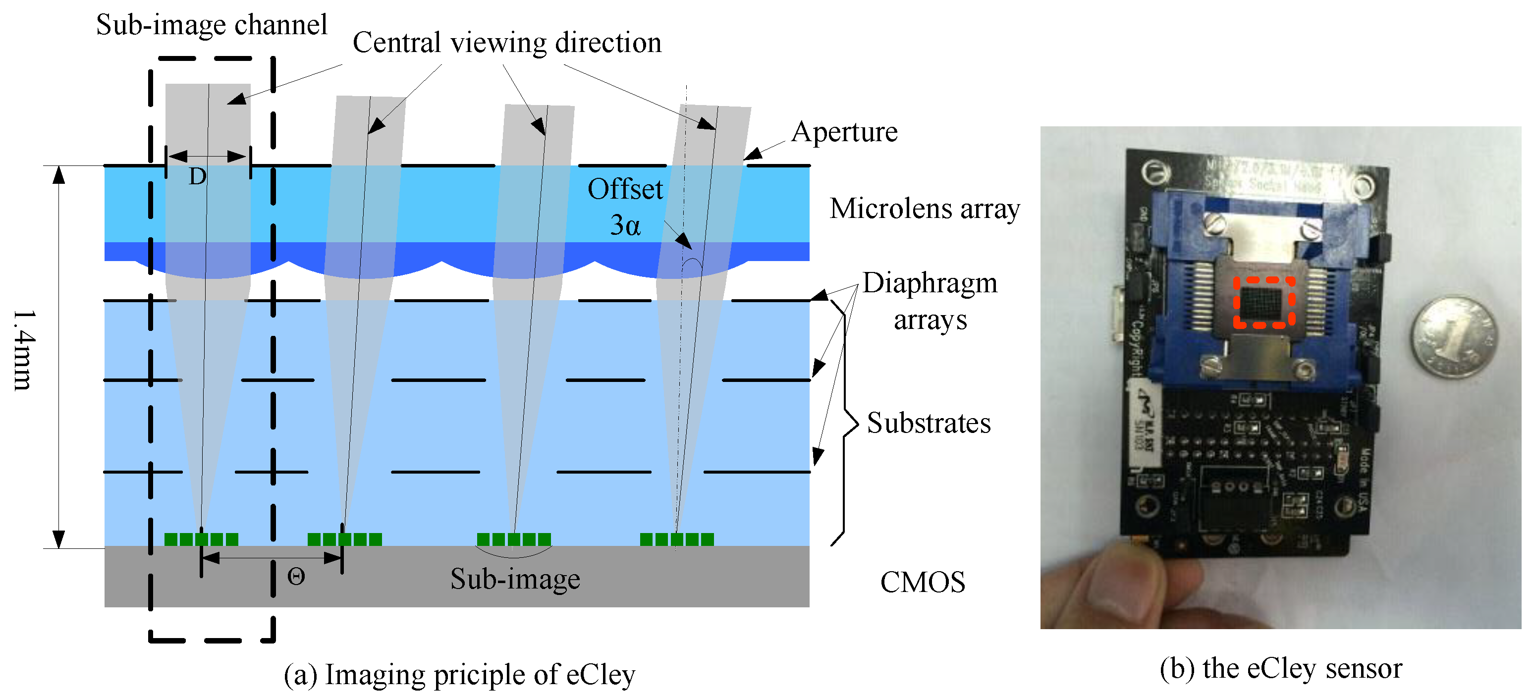
1. Introduction
- The low-resolution and small FOV. In this paper, the rectified sub-image has only pixels, and the FOV of the sub-image is about , which will lead to a large textureless area in the sub-image.
- The large FOV offset. For the eCley, the inherent offset between adjacent sub-images is about 34 pixels, and the overlap area between adjacent images is less than . As shown in Figure 4, Figure 4a gives the target sub-image located in the center and its four neighboring sub-images placed at the corresponding location. Figure 4b–d show the overlap between the target sub-image and each adjacent sub-image, where the green area indicates the non-overlapped area. This will result in much less contextual information being used.
- The photo-consistency may not hold for all pixels. Due to the low resolution and noise, the boundary of objects will be blurred, and the point-wise depth map will be very noisy.
2. Related Work
3. Overview of Edge Matching and Propagation
- Image correction. Because the ACE image suffers distortion, the first step is to rectify sub-images. This will greatly reduce the complexity of the following depth estimation.
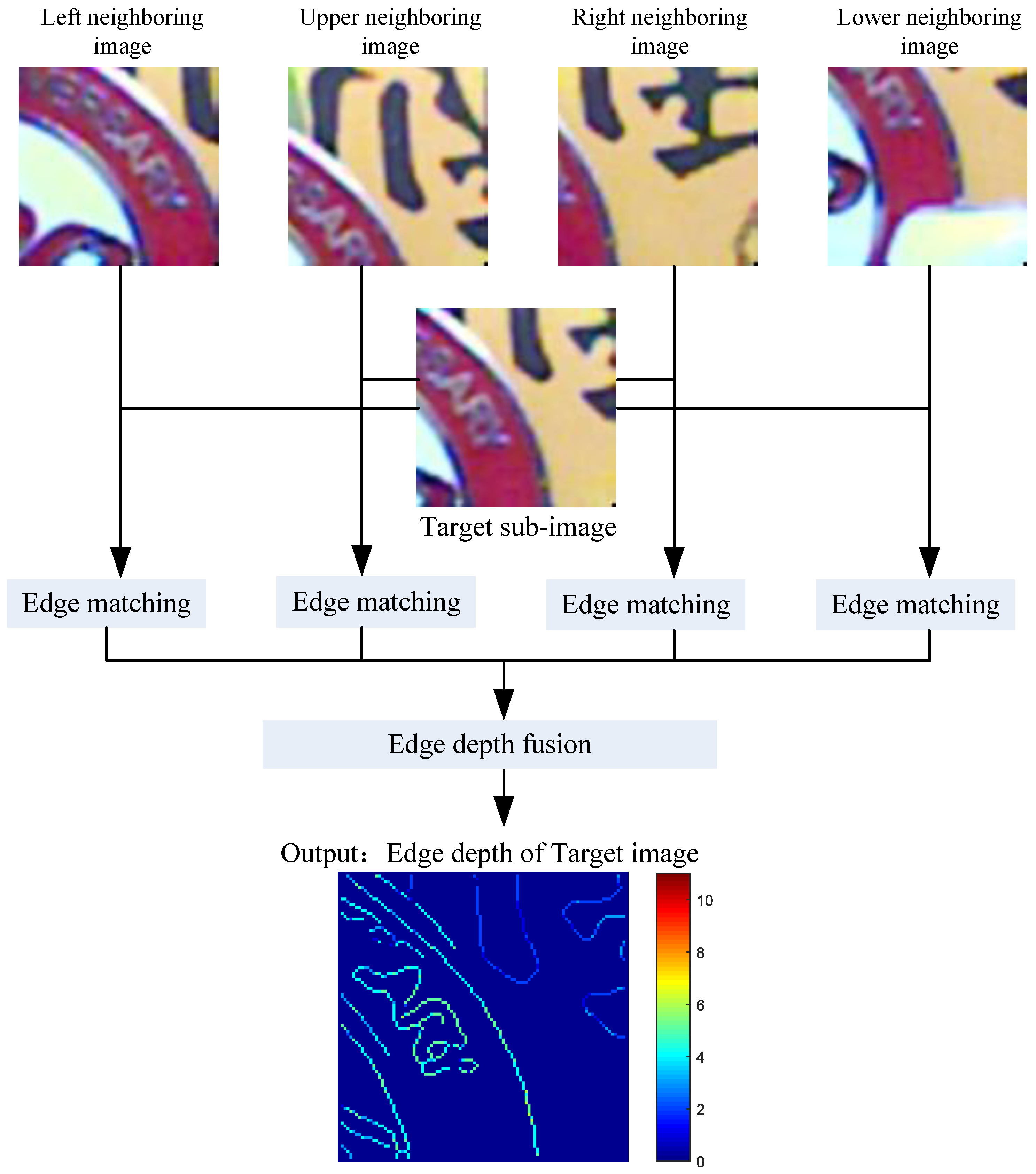
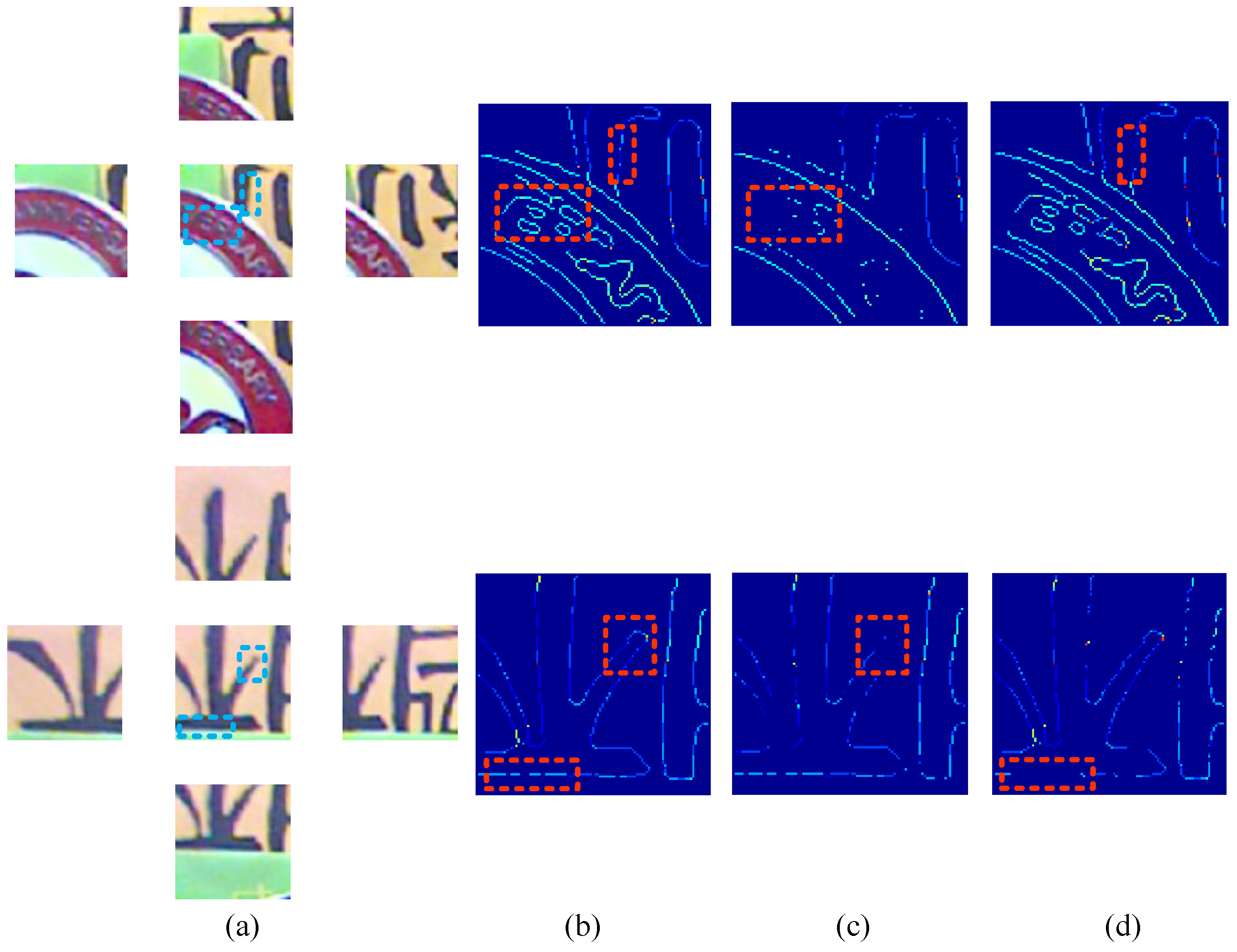
- Edge depth estimation. The inputs to the edge depth estimation module consist of a reference image and four adjacent images, which have been rectified already. The main purpose of this module is to obtain a consistent sparse edge depth map of the reference image.
- Edge depth propagation. The purpose of this module is mainly to propagate the edge depth to the whole image. Associated with over-segmentation results and four neighbor images, this matching cost of the segmented area is much more robust to obtain the correct depth.
- Inconsistency checking and refinement. The main purpose of this module is to identify segmented areas which have unreliable depth. Instead of the left–right check used in many stereo matching algorithms, matching consistency with four neighboring images is used.
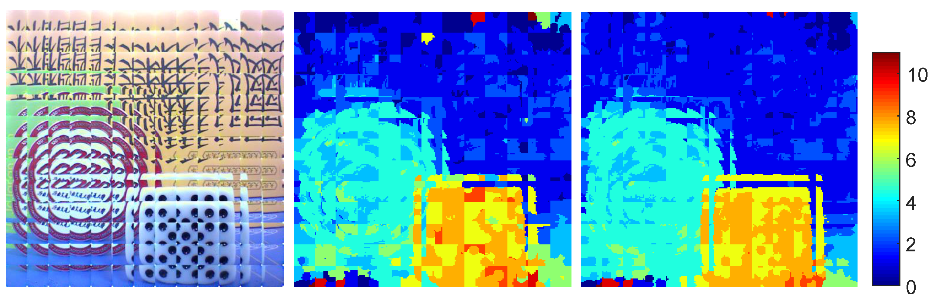
- All-in-focus reconstruction. Finally, based on the refined depth map of each sub-image, the sub-image arrays are rendered to reconstruct the all-in-focus image, and the depth maps are also merged into a whole depth map.
4. Edge Matching and Propagation Method
4.1. Image Correction
4.2. Edge Depth Estimation
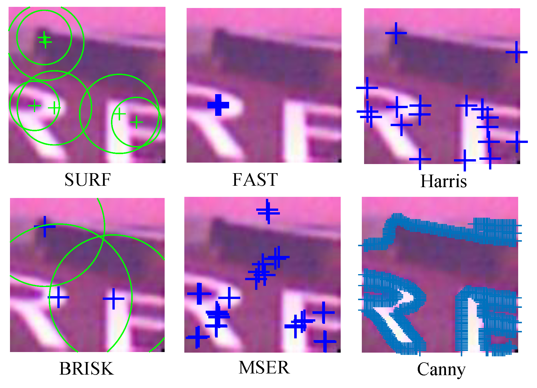
4.2.1. Sub-Image Matching Feature Selection
4.2.2. Edge Feature Matching
4.2.3. Edge Depth Fusion
- The pixel p in the four has the same depth. The depth of remains the same.
- The pixel p in the four has different depths, and the difference is smaller than 2 pixels. The smaller depth is chosen.
- The pixel p in the four has different depths, and the difference is not smaller than 2 pixels. The depth of the pixel is considered unreliable, and is set to 0.
4.3. Edge Depth Propagation
| Algorithm 1 Edge Depth Propagation |
Input: Edge depth map () and color images () Output: Dense depth map
|
4.4. Inconsistency Check and Depth Refinement
4.5. All-in-Focus Reconstruction
5. Experiments
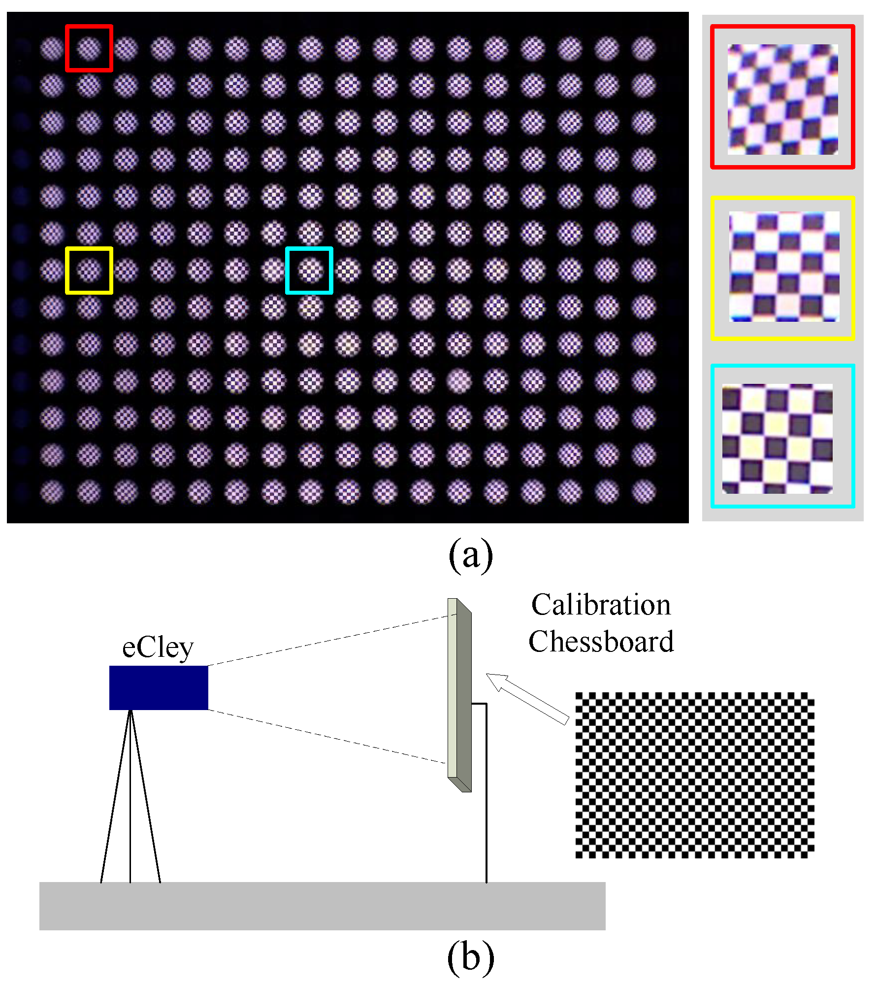
5.1. Experimental Settings
5.2. Evaluation
5.2.1. Image Correction
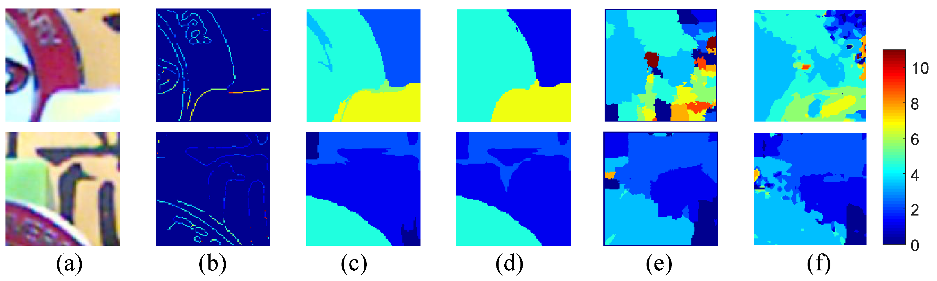
5.2.2. Edge Depth Estimation
5.2.3. Sub-Image Depth
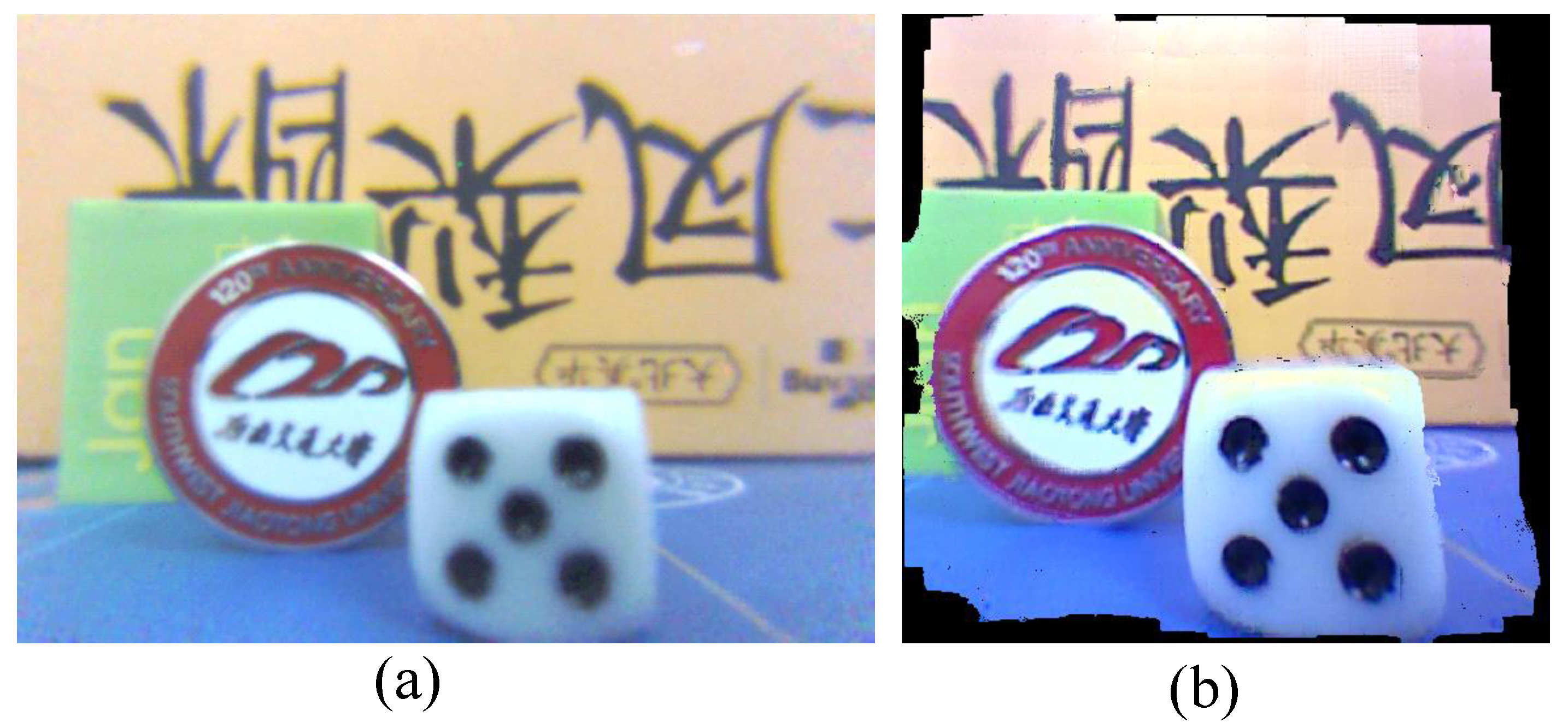
5.2.4. Image Reconstruction
5.2.5. Failure Cases
6. Conclusions
Author Contributions
Funding
Institutional Review Board Statement
Informed Consent Statement
Data Availability Statement
Acknowledgments
Conflicts of Interest
References
- Brückner, A.; Duparré, J.; Leitel, R.; Dannberg, P.; Bräuer, A.; Tünnermann, A. Thin wafer-level camera lenses inspired by insect compound eyes. Opt. Express 2010, 18, 24379–24394. [Google Scholar] [CrossRef]
- Yamada, K.; Mitsui, H.; Asano, T.; Tanida, J.; Takahashi, H. Development of ultra thin three-dimensional image capturing system. In Proceedings of the Three-Dimensional Image Capture and Applications VII; SPIE: San Jose, CA, USA, 2006; Volume 6056, pp. 287–295. [Google Scholar]
- Wu, S.; Jiang, T.; Zhang, G.; Schoenemann, B.; Neri, F.; Zhu, M.; Bu, C.; Han, J.; Kuhnert, K.D. Artificial compound eye: A survey of the state-of-the-art. Artif. Intell. Rev. 2017, 48, 573–603. [Google Scholar] [CrossRef]
- Oberdörster, A.; Brückner, A.; Wippermann, F.C.; Bräuer, A. Correcting distortion and braiding of micro-images from multi-aperture imaging systems. In Proceedings of the Sensors, Cameras, and Systems for Industrial, Scientific, and Consumer Applications XII; SPIE: San Francisco, CA, USA, 2011; Volume 7875, pp. 73–85. [Google Scholar]
- Scharstein, D.; Szeliski, R. A taxonomy and evaluation of dense two-frame stereo correspondence algorithms. Int. J. Comput. Vis. 2002, 47, 7–42. [Google Scholar] [CrossRef]
- Sun, J.; Zheng, N.N.; Shum, H.Y. Stereo matching using belief propagation. IEEE Trans. Pattern Anal. Mach. Intell. 2003, 25, 787–800. [Google Scholar]
- Hirschmuller, H. Stereo processing by semiglobal matching and mutual information. IEEE Trans. Pattern Anal. Mach. Intell. 2007, 30, 328–341. [Google Scholar] [CrossRef] [PubMed]
- Hosni, A.; Rhemann, C.; Bleyer, M.; Rother, C.; Gelautz, M. Fast cost-volume filtering for visual correspondence and beyond. IEEE Trans. Pattern Anal. Mach. Intell. 2012, 35, 504–511. [Google Scholar] [CrossRef] [PubMed]
- Liu, B.; Yu, H.; Long, Y. Local similarity pattern and cost self-reassembling for deep stereo matching networks. Proc. AAAI Conf. Artif. Intell. 2022, 36, 1647–1655. [Google Scholar] [CrossRef]
- Shen, Z.; Dai, Y.; Song, X.; Rao, Z.; Zhou, D.; Zhang, L. PCW-Net: Pyramid combination and warping cost volume for stereo matching. In Proceedings of the European Conference on Computer Vision, Tel Aviv, Israel, 23–27 October 2022; pp. 280–297. [Google Scholar]
- Xu, G.; Wang, X.; Ding, X.; Yang, X. Iterative geometry encoding volume for stereo matching. In Proceedings of the IEEE/CVF Conference on Computer Vision and Pattern Recognition, Vancouver, BC, Canada, 17–24 June 2023; pp. 21919–21928. [Google Scholar]
- Lhuillier, M.; Quan, L. A quasi-dense approach to surface reconstruction from uncalibrated images. IEEE Trans. Pattern Anal. Mach. Intell. 2005, 27, 418–433. [Google Scholar] [CrossRef]
- Zabih, R.; Woodfill, J. Non-parametric local transforms for computing visual correspondence. In Proceedings of the European Conference on Computer Vision, Stockholm, Sweden, 2–6 May 1994; pp. 151–158. [Google Scholar]
- Belongie, S.; Malik, J.; Puzicha, J. Shape matching and object recognition using shape contexts. IEEE Trans. Pattern Anal. Mach. Intell. 2002, 24, 509–522. [Google Scholar] [CrossRef]
- Tanida, J.; Kumagai, T.; Yamada, K.; Miyatake, S.; Ishida, K.; Morimoto, T.; Kondou, N.; Miyazaki, D.; Ichioka, Y. Thin observation module by bound optics (TOMBO): Concept and experimental verification. Appl. Opt. 2001, 40, 1806–1813. [Google Scholar] [CrossRef]
- Duparré, J.; Dannberg, P.; Schreiber, P.; Bräuer, A.; Tünnermann, A. Artificial apposition compound eye fabricated by micro-optics technology. Appl. Opt. 2004, 43, 4303–4310. [Google Scholar] [CrossRef] [PubMed]
- Duparré, J.; Wippermann, F. Micro-optical artificial compound eyes. Bioinspir. Biomim. 2006, 1, R1. [Google Scholar] [CrossRef] [PubMed]
- Brückner, A.; Duparré, J.; Dannberg, P.; Bräuer, A.; Tünnermann, A. Artificial neural superposition eye. Opt. Express 2007, 15, 11922–11933. [Google Scholar] [CrossRef] [PubMed]
- Druart, G.; Guérineau, N.; Haïdar, R.; Lambert, E.; Tauvy, M.; Thétas, S.; Rommeluère, S.; Primot, J.; Deschamps, J. MULTICAM: A miniature cryogenic camera for infrared detection. In Proceedings of the Micro-Optics 2008; SPIE: Strasbourg, France, 2008; Volume 6992, pp. 129–138. [Google Scholar]
- Meyer, J.; Brückner, A.; Leitel, R.; Dannberg, P.; Bräuer, A.; Tünnermann, A. Optical cluster eye fabricated on wafer-level. Opt. Express 2011, 19, 17506–17519. [Google Scholar] [CrossRef] [PubMed]
- Jeong, K.H.; Kim, J.; Lee, L.P. Biologically inspired artificial compound eyes. Science 2006, 312, 557–561. [Google Scholar] [CrossRef] [PubMed]
- Song, Y.M.; Xie, Y.; Malyarchuk, V.; Xiao, J.; Jung, I.; Choi, K.J.; Liu, Z.; Park, H.; Lu, C.; Kim, R.H.; et al. Digital cameras with designs inspired by the arthropod eye. Nature 2013, 497, 95–99. [Google Scholar] [CrossRef] [PubMed]
- Floreano, D.; Pericet-Camara, R.; Viollet, S.; Ruffier, F.; Brückner, A.; Leitel, R.; Buss, W.; Menouni, M.; Expert, F.; Juston, R.; et al. Miniature curved artificial compound eyes. Proc. Natl. Acad. Sci. USA 2013, 110, 9267–9272. [Google Scholar] [CrossRef] [PubMed]
- Lee, G.J.; Choi, C.; Kim, D.H.; Song, Y.M. Bioinspired artificial eyes: Optic components, digital cameras, and visual prostheses. Adv. Funct. Mater. 2018, 28, 1705202. [Google Scholar] [CrossRef]
- Cheng, Y.; Cao, J.; Zhang, Y.; Hao, Q. Review of state-of-the-art artificial compound eye imaging systems. Bioinspir. Biomim. 2019, 14, 031002. [Google Scholar] [CrossRef]
- Kim, M.S.; Kim, M.S.; Lee, G.J.; Sunwoo, S.H.; Chang, S.; Song, Y.M.; Kim, D.H. Bio-inspired artificial vision and neuromorphic image processing devices. Adv. Mater. Technol. 2022, 7, 2100144. [Google Scholar] [CrossRef]
- Kitamura, Y.; Shogenji, R.; Yamada, K.; Miyatake, S.; Miyamoto, M.; Morimoto, T.; Masaki, Y.; Kondou, N.; Miyazaki, D.; Tanida, J.; et al. Reconstruction of a high-resolution image on a compound-eye image-capturing system. Appl. Opt. 2004, 43, 1719–1727. [Google Scholar] [CrossRef] [PubMed]
- Nitta, K.; Shogenji, R.; Miyatake, S.; Tanida, J. Image reconstruction for thin observation module by bound optics by using the iterative backprojection method. Appl. Opt. 2006, 45, 2893–2900. [Google Scholar] [CrossRef] [PubMed]
- Horisaki, R.; Irie, S.; Ogura, Y.; Tanida, J. Three-dimensional information acquisition using a compound imaging system. Opt. Rev. 2007, 14, 347–350. [Google Scholar] [CrossRef]
- Horisaki, R.; Nakao, Y.; Toyoda, T.; Kagawa, K.; Masaki, Y.; Tanida, J. A thin and compact compound-eye imaging system incorporated with an image restoration considering color shift, brightness variation, and defocus. Opt. Rev. 2009, 16, 241–246. [Google Scholar] [CrossRef]
- Dobrzynski, M.K.; Pericet-Camara, R.; Floreano, D. Vision Tape—A flexible compound vision sensor for motion detection and proximity estimation. IEEE Sens. J. 2011, 12, 1131–1139. [Google Scholar] [CrossRef]
- Luke, G.P.; Wright, C.H.; Barrett, S.F. A multiaperture bioinspired sensor with hyperacuity. IEEE Sens. J. 2010, 12, 308–314. [Google Scholar] [CrossRef]
- Prabhakara, R.S.; Wright, C.H.; Barrett, S.F. Motion detection: A biomimetic vision sensor versus a CCD camera sensor. IEEE Sens. J. 2010, 12, 298–307. [Google Scholar] [CrossRef]
- Gao, Y.; Liu, W.; Yang, P.; Xu, B. Depth estimation based on adaptive support weight and SIFT for multi-lenslet cameras. In Proceedings of the 6th International Symposium on Advanced Optical Manufacturing and Testing Technologies: Optoelectronic Materials and Devices for Sensing, Imaging, and Solar Energy; SPIE: Xiamen, China, 2012; Volume 8419, pp. 63–66. [Google Scholar]
- Park, S.; Lee, K.; Song, H.; Cho, J.; Park, S.Y.; Yoon, E. Low-power, bio-inspired time-stamp-based 2-D optic flow sensor for artificial compound eyes of micro air vehicles. IEEE Sens. J. 2019, 19, 12059–12068. [Google Scholar] [CrossRef]
- Agrawal, S.; Dean, B.K. Edge detection algorithm for Musca-Domestica inspired vision system. IEEE Sens. J. 2019, 19, 10591–10599. [Google Scholar] [CrossRef]
- Lee, W.B.; Lee, H.N. Depth-estimation-enabled compound eyes. Opt. Commun. 2018, 412, 178–185. [Google Scholar] [CrossRef]
- Oberdörster, A.; Brückner, A.; Wippermann, F.; Bräuer, A.; Lensch, H.P. Digital focusing and refocusing with thin multi-aperture cameras. In Proceedings of the Digital Photography VIII; SPIE: BBurlingame, CA, USA, 2012; Volume 8299, pp. 58–68. [Google Scholar]
- Ziegler, M.; Zilly, F.; Schaefer, P.; Keinert, J.; Schöberl, M.; Foessel, S. Dense lightfield reconstruction from multi aperture cameras. In Proceedings of the 2014 IEEE International Conference on Image Processing (ICIP), Paris, France, 27–30 October 2014; pp. 1937–1941. [Google Scholar]
- Jiang, T.; Zhu, M.; Kuhnert, K.D.; Kuhnert, L. Distance measuring using calibrating subpixel distances of stereo pixel pairs in artificial compound eye. In Proceedings of the 2014 International Conference on Informative and Cybernetics for Computational Social Systems (ICCSS), Qingdao, China, 9–10 October 2014; pp. 118–122. [Google Scholar]
- Wu, S.; Zhang, G.; Zhu, M.; Jiang, T.; Neri, F. Geometry based three-dimensional image processing method for electronic cluster eye. Integr. Comput. Aided Eng. 2018, 25, 213–228. [Google Scholar] [CrossRef]
- Wu, S.; Zhang, G.; Neri, F.; Zhu, M.; Jiang, T.; Kuhnert, K.D. A multi-aperture optical flow estimation method for an artificial compound eye. Integr. Comput. Aided Eng. 2019, 26, 139–157. [Google Scholar] [CrossRef]
- Javidi, B.; Carnicer, A.; Arai, J.; Fujii, T.; Hua, H.; Liao, H.; Martínez-Corral, M.; Pla, F.; Stern, A.; Waller, L.; et al. Roadmap on 3D integral imaging: Sensing, processing, and display. Opt. Express 2020, 28, 32266–32293. [Google Scholar] [CrossRef] [PubMed]
- Wu, G.; Masia, B.; Jarabo, A.; Zhang, Y.; Wang, L.; Dai, Q.; Chai, T.; Liu, Y. Light field image processing: An overview. IEEE J. Sel. Top. Signal Process. 2017, 11, 926–954. [Google Scholar] [CrossRef]
- Bay, H.; Tuytelaars, T.; Van Gool, L. Surf: Speeded up robust features. In Proceedings of the European Conference on Computer Vision, Graz, Austria, 7–13 May 2006; pp. 404–417. [Google Scholar]
- Rosten, E.; Drummond, T. Fusing points and lines for high performance tracking. In Proceedings of the IEEE International Conference on Computer Vision, Beijing, China, 17–21 October 2005; Volume 2, pp. 1508–1515. [Google Scholar]
- Harris, C.; Stephens, M. A combined corner and edge detector. In Proceedings of the Alvey Vision Conference, Manchester, UK, 31 August–2 September 1988; Volume 15, pp. 147–152. [Google Scholar]
- Leutenegger, S.; Chli, M.; Siegwart, R.Y. BRISK: Binary robust invariant scalable keypoints. In Proceedings of the IEEE International Conference on Computer Vision, Barcelona, Spain, 6–13 November 2011; pp. 2548–2555. [Google Scholar]
- Mikolajczyk, K.; Tuytelaars, T.; Schmid, C.; Zisserman, A.; Matas, J.; Schaffalitzky, F.; Kadir, T.; Gool, L.V. A comparison of affine region detectors. Int. J. Comput. Vis. 2005, 65, 43–72. [Google Scholar] [CrossRef]
- Canny, J. A computational approach to edge detection. IEEE Trans. Pattern Anal. Mach. Intell. 1986, PAMI-8, 679–698. [Google Scholar] [CrossRef]
- Comaniciu, D.; Meer, P. Mean shift: A robust approach toward feature space analysis. IEEE Trans. Pattern Anal. Mach. Intell. 2002, 24, 603–619. [Google Scholar] [CrossRef]
- Levin, A.; Lischinski, D.; Weiss, Y. A closed-form solution to natural image matting. IEEE Trans. Pattern Anal. Mach. Intell. 2007, 30, 228–242. [Google Scholar] [CrossRef] [PubMed]
- Zuo-Lin, L.; Xiao-hui, L.; Ling-Ling, M.; Yue, H.; Ling-li, T. Research of definition assessment based on no-reference digital image quality. Remote Sens. Technol. Appl. 2011, 26, 239–246. [Google Scholar]


| Feature | SURF | FAST | Harris | BRISK | MSER | Canny |
|---|---|---|---|---|---|---|
| Count | 6 | 1 | 18 | 3 | 32 | 554 |
| eCley Image | Metrics | Sub-Image 1 | Sub-Image 2 | Sub-Image 3 |
|---|---|---|---|---|
| BP [6] 2003 | MSE | 0.0823 | 0.0593 | 0.0766 |
| 2732 | 1910 | 1783 | ||
| 11682 | 7427 | 11386 | ||
| 665 | 367 | 489 | ||
| 3982 | 2417 | 3142 | ||
| Cost Filter [8] 2012 | MSE | 0.0843 | 0.0654 | 0.0829 |
| 2662 | 1821 | 1704 | ||
| 10821 | 7309 | 10923 | ||
| 587 | 321.4 | 501 | ||
| 3811 | 2398.2 | 3028.7 | ||
| G3D [41] 2018 | MSE | 0.048 | 0.0536 | 0.0535 |
| 2883 1 | 1987.2 | 1847 | ||
| 11861 | 7654.5 | 11556 | ||
| 684.4 | 385 | 519.8 | ||
| 4099 | 2501.8 | 3179.8 | ||
| EdMP [this work] 2024 | MSE | 0.0412 | 0.0507 | 0.0476 |
| 2520 | 2288.1 | 2045 | ||
| 16,446 | 11,983 | 17,116 | ||
| 463.6 | 622.7 | 648.9 | ||
| 3105 | 3273.8 | 3522.7 |
| Method | EdMP | Cost Filter | BP | G3D |
|---|---|---|---|---|
| Time (s) | 180.24 | 197.92 | 312.77 | 169.53 |
Disclaimer/Publisher’s Note: The statements, opinions and data contained in all publications are solely those of the individual author(s) and contributor(s) and not of MDPI and/or the editor(s). MDPI and/or the editor(s) disclaim responsibility for any injury to people or property resulting from any ideas, methods, instructions or products referred to in the content. |
© 2024 by the authors. Licensee MDPI, Basel, Switzerland. This article is an open access article distributed under the terms and conditions of the Creative Commons Attribution (CC BY) license (https://creativecommons.org/licenses/by/4.0/).
Share and Cite
Wu, S.; Ren, L.; Yang, Q. All-in-Focus Three-Dimensional Reconstruction Based on Edge Matching for Artificial Compound Eye. Appl. Sci. 2024, 14, 4403. https://doi.org/10.3390/app14114403
Wu S, Ren L, Yang Q. All-in-Focus Three-Dimensional Reconstruction Based on Edge Matching for Artificial Compound Eye. Applied Sciences. 2024; 14(11):4403. https://doi.org/10.3390/app14114403
Chicago/Turabian StyleWu, Sidong, Liuquan Ren, and Qingqing Yang. 2024. "All-in-Focus Three-Dimensional Reconstruction Based on Edge Matching for Artificial Compound Eye" Applied Sciences 14, no. 11: 4403. https://doi.org/10.3390/app14114403
APA StyleWu, S., Ren, L., & Yang, Q. (2024). All-in-Focus Three-Dimensional Reconstruction Based on Edge Matching for Artificial Compound Eye. Applied Sciences, 14(11), 4403. https://doi.org/10.3390/app14114403