1. Introduction
Urban projections until 2050 [
1] show an increased concentration of population in urban areas. This scenario presents challenges in terms of mobility and traffic that aim to efficiently and sustainably manage resources to increase the quality of life. There are many approaches behind the concept of smart mobility [
2,
3,
4]:
the use of technologies that provide helpful information (IoT, sensors, network);
the creation of structures that include smart roads and monitoring platforms;
the reduction of the ecological footprint (energy saving, bike lanes, etc.).
However, most solutions rely on efficient and accurate navigation processes.
The development of advanced driver assistance systems (ADAS) for connected and automated mobility makes the accuracy [
5] of the navigation process a key issue. Sensors involved in the process of perception and comprehension of the environment, as well as fusion algorithms and decision-makers, have played a significant and evolving role in recent years. Nowadays, many resources provide helpful information to determine position, orientation, time or velocity. Nevertheless, some scenarios and phenomena directly affect the performance of sensor technologies. Thus, it is essential to develop architectures that use a multi-sensor and redundant approach to mitigate the adverse effects caused by the temporary under-performance of one or several sensors.
Recently, proposed architectural solutions have concentrated on sensor fusion [
6,
7] rather than implementing the entire On Board Unit (OBU) system [
8,
9,
10,
11,
12]. This work addresses the fusion process as the core element of the OBU, dedicating a complete architectural layer. The elements used as sensors in our implementation are the inertial measurement unit (IMU) and the global navigation satellite system (GNSS) receiver, complemented by a GNSS augmentation system.
The primary obstacle in enabling AV navigation lies in establishing a consistently accurate and dependable navigation solution across all landscapes. GNSS stands out as the most prevalent source of navigation solutions due to its enduring stability in offering long–term solutions [
13].
However, GNSS encounters limitations in providing accurate or any navigation solution in certain circumstances, notably within urban settings that include tunnels, underground parking areas, and high-rise buildings [
14,
15,
16]. Satellite navigation in the urban environment is subject to some objectively critical issues, mainly related to the following items.
Satellite visibility: due to the presence of urban canyons, the number of visible satellites, crucial for obtaining an accurate position, is limited.
Multipath and non–line–of–sight reception: the typicality and singularity of the urban context, in which the vehicles carry out their service, produces a non–trivial multipath error that seriously compromises the performance of the GNSS signal.
Other kinds of interference that can have a significant impact in an urban context.
These criticalities result in considerable variability in the reception of the GNSS signal, ranging from optimal conditions to complete absence. On the other hand, inertial navigation systems (INS) possess several advantages. They operate continuously, exhibit low short-term noise, and resist jamming and interference. However, INS accuracy degrades over time due to integration errors, and maintaining effective sole-means navigation is costly. While GNSS ensures high long-term accuracy, its output rate is lower, and signal obstruction leads to discontinuous navigation. By integrating INS and GNSS, their advantages complement each other. GNSS measurements prevent inertial solution drift, while INS smoothes GNSS output and bridges signal outages. This integration results in a continuous, high-bandwidth navigation solution with long and short-term accuracy [
17].
The navigation system emerges as a pivotal enabling factor within the framework of the EMERGE project [
18], co-funded by the European Union and spearheaded by RadioLabs in collaboration with esteemed partners such as the University of L’Aquila, Telespazio, Leonardo, and Elital. The project aims to design and develop a novel OBU to provide dual use capabilities to commercial vehicles (i.e., last mile delivery and emergency operations) enabled by dedicated cloud-edge services. The OBU is equipped with vehicle-to-everything (V2X) connectivity [
19], procedures for cyber-secure operations [
20] and an accurate geo-localization platform. The role of this latter is to guarantee real-time, precise positioning of all nodes and their relative positions, accomplished through innovative fusion techniques that leverage data from multi-constellation GNSS sensors and inertial sensors.
When elements with different characteristics regarding data rate, coding, data type, and time references are integrated, an infrastructure capable of handling all the information flows must be designed. For this reason, this work continues in
Section 2, describing an architectural proposal applied in the OBU realisation process. Also, a multi-sensor approach is employed, consequently using data fusion techniques to achieve accurate and robust navigation in different scenarios.
Section 3 details the integration algorithm based on an Extended Kalman Filter. The experimental setup is divided into two parts: one dedicated to evaluating the individual sensors’ performance and the other to evaluating the whole system’s performance based on the integration algorithm.
Section 4 describes the experimentation procedure, and the main results obtained are presented in
Section 5. Finally,
Section 6 concludes this article.
2. EMERGE Onboard System Architecture
This section describes the proposed architecture for achieving the EMERGE On board Unit (OBU). The objective is to present and use a generic architecture: easy to understand and implement, with a scalable structure compatible with different hardware platforms and operating systems. In this sense, the challenge is to define a harmonious level of abstraction that guarantees the following functionalities.
Compatibility: taking advantage of existing components, both: HW and SW (COTS).
Efficiency: exploiting the advantage of the HW architecture used.
Performance: establishment of specific metrics in each context.
Portability: to guarantee compatibility with Operating Systems and HW.
Operation: real-time or post-processing execution capability.
Scalability: add/delete components: Sensors, SW, algorithms.
We highlight the proposal of five specified layers based on their functionality and interaction with the navigation system. Including a monitoring layer allows the evaluation of prototypes and different scenarios, the detection of anomalies and problems in the singular components of the system and the evaluation of performances.
Figure 1 shows the diagram of the proposed architecture. Each of the layers to which each element belongs is identified by a different colour. The connections, paths and formats/encoding used by each element of the OBU are specified. Below, some details of the functional blocks are presented.
Sensor (layer 1): includes all sensors capable of providing helpful information in the navigation process, i.e., GNSS receivers, inertial sensors, RTK stations, augmentation services, onboard sensors, and external clocks.
Parser; Conditioner (layer 2): handles decoding/parsing and filtering information from the sensor level. When communication with sensors (configuration signals, request) is needed, this block also implements the appropriate coding/decoding process.
Controller (layer 3): controls the start-up, interruptions, restart, and the change of parameters process (in the case of a dynamic scenario). In addition, it manages the possible changes in information flows that may occur between the Core layer and the Sensor layer.
Core (layer 4): The system’s centre contains all the navigation and information management algorithms. In this application, the Sensor Fusion algorithm and the Integrity SW components are located in this layer.
Monitoring (layer 5): This layer monitors the system’s performance in the navigation process and HW resources. It also introduces remote accessibility functionalities and possibly warning signals and notifications.
The proposed blocks or components in each layer are intended to provide the required functionalities of the OBU. The first element to guarantee is connectivity (“always connected”). The OBU COMM and CRYPTO ENGINE blocks are external subsystems ensuring remote communication and IP-based services access. The system uses the connection to receive information from the Augmentation GNSS (AGNSS) systems and exchange information with traffic control elements: control centres, other vehicles, or early alert systems. The system proposes solutions based on loosely coupled integration between the inertial sensor measurements and the previously corrected GNSS navigation solutions. The modules involved in the navigation process are dedicated to decoding the information coming from the sensors, managing the information flows and synchronisation. The main objective is to integrate or fuse all useful navigation information to achieve higher levels of accuracy and integrity.
2.1. EMERGE Navigation System Implementation
The HW, SW or service components that drive up the onboard navigation system are selected according to the functional requirements of the EMERGE project. For each use case, requirements are mapped to performance measures that sensors must satisfy in the first layer. Specifically, two main elements are considered: the GNSS receiver and the inertial sensor. A GNSS augmentation service is used to improve the satellite positioning performance through corrections received via the OBU connection to the Internet.
2.1.1. Sensors and Services
The GNSS receiver uses the u-blox ZED-F9P positioning module [
21] that provides multi-band GNSS for high-volume industrial applications. The ZED-F9P integrates multi-band RTK and PPP-RTK (Precise Point Positioning—Real Time Kinematic) for centimetre accuracy. The module is ideal for automotive and UAV applications due to its low power consumption, accuracy and integration capability. Another strength of this receiver is the ability to handle multiple channels dedicated to different constellations and frequency bands. In addition, the ZED-F9P module features native compatibility with the PointPerfect (PP) augmentation service [
22].
PointPerfect is a GNSS augmentation service that supports PPP-RTK for position estimation, with 99.9% availability using the Internet or satellite (L-band) connection. The PP service has reported high availability and high levels of accuracy, making this product optimal for critical applications such as automotive. Specifically, in our configuration, we receive corrections over an IP connection. The GNSS corrections are received in SPARTN 2.0 format transparently and cost-effectively via the MQTT broker offered by the u-blox Thingstream platform [
23]. This method of receiving GNSS corrections ensures efficient use of bandwidth, improves GNSS receiver initialisation times and reduces the power consumption of the navigation system. It is important to note that the specific PointPerfect IP service (Unlimited access to IP data stream) costs 19.00 USD per month at the moment of this research.
The inertial sensor component used is the Xsens-MTi-630 AHRS (Attitude and Heading Reference System) [
24], which contains a 3-axis gyroscope, a 3-axis accelerometer, a 3-axis barometer magnetometer, a high-precision oscillator and a low-power microcontroller unit (MCU). The MCU applies calibration models (unique to each sensor and including orientation, gain and polarisation offsets, plus more advanced relationships such as non-linear temperature effects and other higher order terms) and runs Xsens’ optimised strap-down algorithm, which performs high-speed dead-reckoning calculations up to 2 kHz, enabling accurate capture of high-frequency motions and compensation for coning and sculling. The MTi-600’s output data is easily configured and customised according to the application’s requirements and can be set to use one of several inertial navigation filter profiles [
25]. In particular, the MTi-630 AHRS device enhances the process of determining referenced magnetic north and 3D acceleration, velocity and heading calibration data. The project requirements motivating the use of this sensor are low in-run bias stability (accelerometer: 10 (x,y) and 15 (z) [micro-g]; gyroscope: 8 [deg/h]), low noise density (accelerometers: 60 [micro-g/sqrt(Hz)]) and the ability to output data at a sufficiently high frequency for the sensor fusion process. Successive models of the MTi-600 family (i.e., MTi-670/80) support the INS/GNSS integration process internally; in our case, they do not; therefore, the INS/GNSS synchronisation and integration process is performed by SW.
2.1.2. Sensor Fusion and Integrity
The navigation system’s core comprises the components in charge of PNT (Positioning, Navigation and Timing) and Integrity estimation. The multi-sensor approach uses an algorithm that integrates all the elements that provide helpful information in the navigation process.
Section 3 describes the loosely coupled algorithm that integrates inertial and GNSS data.
2.1.3. Signal and Information Exchange
The
Always Connected paradigm opens up many possibilities and functionalities for the satellite navigation system. Therefore, a communication system between internal and external elements is essential. We use MQTT as a communication protocol to guarantee agile and lightweight internal communication between the OBU components (sensors, SW modules, monitoring services). MQTT is a standards-based communication protocol [
26], or set of rules, used to communicate from one device/sensor/component to another. Intelligent sensors, wearable devices, and other IoT elements typically transmit and receive data that require modest bandwidth. Therefore, MQTT is used for data exchange as it is easy to implement and can communicate data efficiently.
Figure 2 presents a detailed view of exchanging messages via the MQTT broker (Identified as “SBC BROKER”). The arrowheads on the individual connections show whether it is only a subscriber, publishes and subscribes, or only publishes messages through the Broker. For instance, given its observation functionality, the Monitoring block only intends to receive messages and not publish them. Sensors and services publish correctly decoded measured/acquired data in a dedicated Topic, from where they are accessible to the processes or modules that process them. The
Controller4Controllers module is responsible for configuring, calibrating and synchronising the sensors and coding/decoding SW components. The Broker is also involved in the external communication process via the
OBU COMM module. After the appropriate encryption process, the information to be transmitted to the control centre is made available in a dedicated Topic managed by the Data Management element.
2.1.4. Power Management System
The Power Management System is the element that ensures that the system stays on and continues to operate regardless of the state of the vehicle. It consists of two elements: a HW and a SW element. The HW element is the Sixfab Power Management; UPS HAT [
27], while the SW element is implemented using a dedicated API: Sixfab Power Python API [
28]. In short, it is an uninterruptible power supply with a built-in 18650-Li-Ion battery, allowing it to automatically switch from one power supply to another without causing a reboot or system failure. The device can enter deep sleep mode in power-sensitive applications and save battery energy.
2.1.5. Monitoring
The Monitoring component consists of a Frontend, a graphical interface that displays the data of interest, and a Backend responsible for manipulating and storing internal and external information flows. This project’s Monitoring layer is based on the Node-RED [
29] tool or framework. Node-RED is a flow-based development tool developed to connect devices, APIs and online services as part of the IoT. In addition, it provides a web browser-based flow editor, which can be used to create JavaScript functions. Application elements can be saved or shared for reuse. The runtime uses Node.js, and the streams created are stored using JSON. The decision to use this technology is based on simplicity and support for the MQTT protocol and sensor information. In addition, the built-in WEB service allows remote monitoring of the system.
2.1.6. Hardware Description
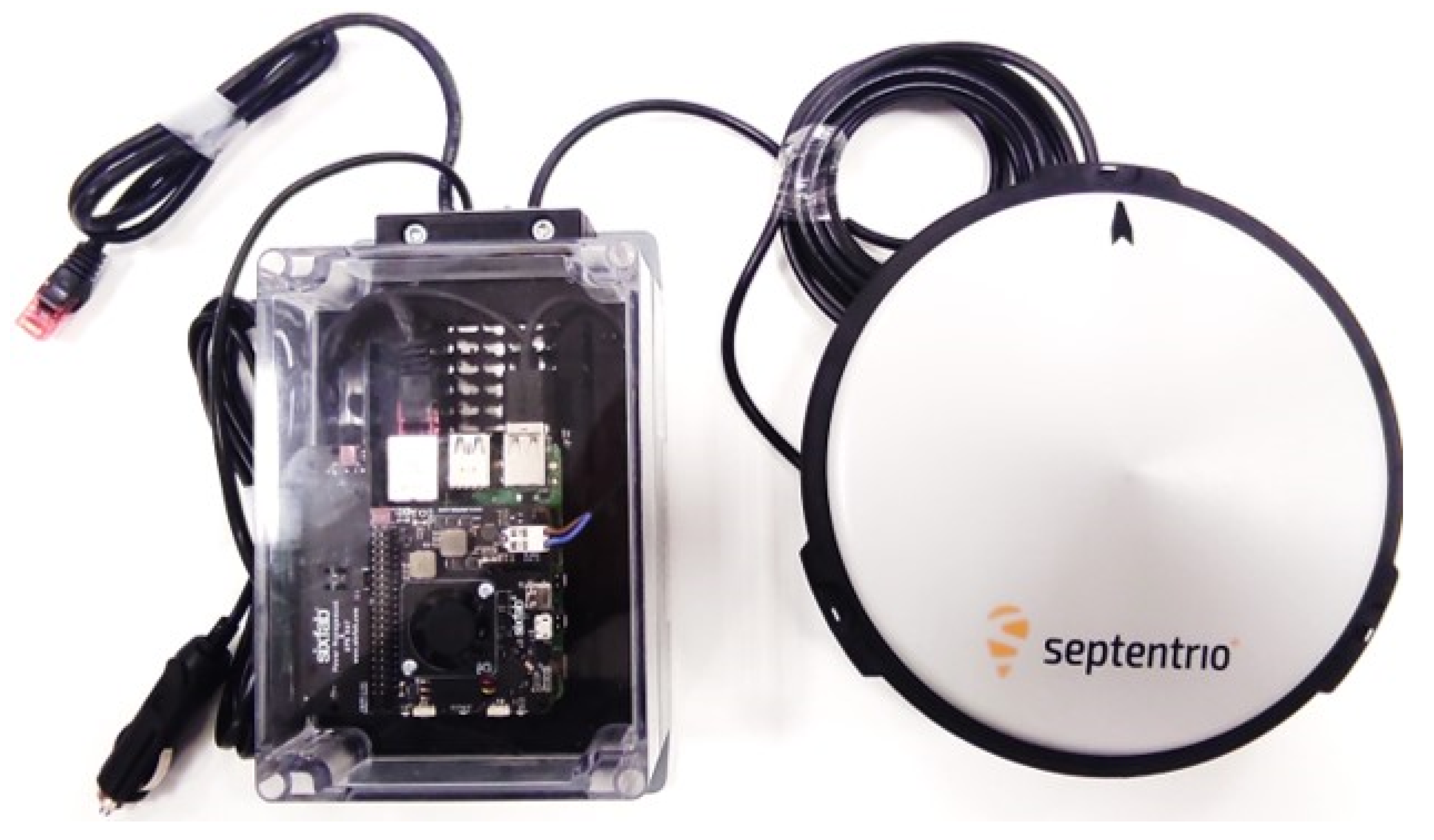
The HW used as the On–Board Computer (OBC), shown in
Figure 3, is the Raspberry Pi 4 Model B [
30] equipped with BCM2711, quad–core Cortex–A72 (ARM v8) 64–bit SoC @ 1.8 GHz, 8 GB SDRAM memory and 32 GB Micro–SD card. The sensors (Inertial and GNSS) are connected via USB interfaces, while the Power Management and UPS system is connected to the standard 40-pin GPIO. The SIRIUS RTK GNSS ROVER multi–constellation receiver [
31] (based on u–blox ZED-F9P) is connected to the Septentrio Polant–x MF antenna via the SMA interface provided. Both the antenna and the GNSS receiver verify multi–frequency and multi–constellation compatibility. Finally, the components are assembled inside a Sixfab enclosure specifically dedicated to Raspberry projects in outdoor environments with IP65 compliance. An IP65–rated enclosure gives protection against moisture, rain, snow, wind, dust and low–pressure water jets from any direction, as well as condensation and water spray. It is suitable for most outdoor enclosures that will not encounter extreme weather.
Figure 4 shows the final Navigation Box, the interfaces and the GNSS antenna.
3. Sensor Fusion: Loosely Coupled Algorithm Implementation
The primary advantage of a loosely coupled integration architecture lies in its simplicity. This architecture is versatile and compatible with any INS and GNSS user equipment, making it ideal for retrofit applications. In a loosely coupled INS/GNSS system, the integration algorithm utilizes GNSS position and velocity solutions as measurement inputs, regardless of the specific type of INS correction or GNSS aiding employed.
In the cascaded operation of this architecture, the GNSS user equipment, which incorporates a navigation filter [
17], utilizes the Extended Kalman Filter (EKF) as the integration solution. The EKF is a recursive filter specifically designed to estimate the state of a dynamic system from multiple noisy measurements. It has evolved from the Standard Kalman Filter to address the complexities associated with nonlinear dynamic systems. The resulting integrated navigation solution consists of the INS navigation solution refined by the Kalman filter’s error estimates. Specifically, within the loosely coupled integration architecture, the sequential processes can be delineated as follows:
calculation of position and velocity with GNSS;
calculation of the difference between the estimated position and velocity from the GNSS and INS solutions to assess IMU errors by integrating the estimated differences in a Kalman filter;
correction of the INS solution using variational equations.
The tests were carried out in a confined area. To simplify the spatial representation in this local context, the North East Down (NED) coordinate frame was chosen. Consequently, the position of the OBU is represented using geodetic coordinates: latitude , longitude , and ellipsoidal altitude . The Earth-referenced velocity is resolved in the local navigation axis to give , and the attitude is expressed as the body-to-local navigation frame coordinate transformation matrix . Here, e denotes the Earth-Centered Earth-Fixed (ECEF) reference frame, n is the NED frame, and b represents the inertial platform “body” coordinate frame.
Figure 5 illustrates the functional diagram of the GNSS-INS loose coupling process. It is a closed-loop correction architecture; consequently, the estimated errors in the NED reference frame,
for the latitude,
for the longitude,
for the height,
for the velocity and
for the attitude are fed back to the inertial navigation processor, where they are used to correct the inertial navigation solution. In this way, the integrated navigation solution of the navigation system is the inertial navigation solution itself, and is obtained, respectively, for the orientation,
, the velocity,
, and the position, as follows [
17]:
where superscripts − and + are used to indicate the solution before and after correction,
is the vector of Euler angles of the correction (i.e., yaw, pitch, and roll), and
represents the antisymmetric matrix
The pseudocode outlined in Algorithm 1 presents the procedural steps of the implemented INS-GNSS loosely coupled algorithm. Initially, it sets crucial parameters to account for IMU errors. The algorithm then begins with an initialisation loop which is used to estimate the initial pose of the vehicle and to configure Kalman filter parameters. After initialisation, it uses IMU data to update the vehicle’s pose, incorporating corrections from the Kalman filter when new GNSS measurements are available and providing the integrated navigation solution as output. A Zero Velocity Update (ZUPT) is also employed to mitigate the position drift introduced when the vehicle is stationary. All these steps are further described in the following.
| Algorithm 1 Loosely coupled algorithm |
- 1:
Set initialisation parameters for IMU errors; - 2:
= 100; - 3:
init_time = 15; - 4:
init_imu_samples = init_time * ; - 5:
level_time = 10; - 6:
init_imu_samples_level = level_time * ; - 7:
for to do - 8:
Initialisation loop - 9:
end for - 10:
for to end do - 11:
Specific force ; - 12:
Angular velocity ; - 13:
Correct and using estimated biases; - 14:
Update navigation solution with mechanisation equations; - 15:
Apply ZUPT detection algorithm; - 16:
if There are new solution from GNSS then - 17:
Apply Kalman Filter; - 18:
Update the navigation solution with Kalman filter estimates; - 19:
end if - 20:
end for
|
3.1. Setting Initialisation Parameters for IMU Errors
Inertial navigation systems are renowned for delivering highly accurate position, velocity, and attitude information, particularly over short time spans. However, this precision degrades significantly over extended periods due to inherent error sources within the sensors. To address this challenge, the algorithm’s first step focuses on precisely defining the initialisation parameters related to IMU errors. This meticulous calibration lays the groundwork for mitigating sensor inaccuracies and ensures the subsequent integration of INS-GNSS data yields precise and reliable navigation estimates.
The Allan variance method is used to characterise various error types present in inertial sensor data. This method allows for representing root mean square (RMS) random drift error as a function of averaging time [
32]. Inertial measurements were analysed using the Allan variance method; precisely, specific force and angular velocity measurements collected from the IMU during a stationary five-hour test were utilized. These measurements were crucial in deriving parameters such as velocity random walk, angle random walk, angle rate random walk, bias instability, correlation times, and dynamic bias root–PSD for the accelerometer and gyroscope.
3.2. The Initialisation Loop
As a systematic iteration over IMU samples, this Loop (2) calculates essential parameters and initializes the navigation solution when the system is stationary. Its execution sets the stage for optimal accuracy and performance of the Kalman filter during subsequent integration, establishing a robust foundation for a precise and reliable navigation solution. Within each iteration over the IMU measurement taken in the first seconds, the initialisation loop calculates the IMU sampling interval (
) considering the IMU frequency, facilitating precise temporal alignment. Specific force (
) and angular velocity (
) measurements are extracted from the IMU, providing essential motion-related data. The Algorithm 2 checks for the availability of new GNSS measurements within the current Inertial Navigation System (INS) time. If available, it updates the GNSS position. To account for synchronisation issues between the IMU and GNSS data, this check is performed within a time window of duration
ns. IMU measurements are accumulated for levelling purposes and also GNSS data, when available, is accumulated to initialize position parameters. Roll and pitch are computed based on the averaged specific force measurements through the levelling process. The estimated position is initialized using the averaged GNSS positions.
| Algorithm 2 Initialisation Loop |
- 1:
= ; %duration in seconds - 2:
for to do - 3:
if then - 4:
- 5:
else - 6:
- 7:
end if - 8:
- 9:
- 10:
- 11:
- 12:
- 13:
%Check if there is a new GNSS measurement to process at current INS time - 14:
if then - 15:
- 16:
- 17:
gnss position - 18:
end if - 19:
- 20:
- 21:
if then - 22:
; - 23:
end if - 24:
- 25:
if then - 26:
- 27:
- 28:
- 29:
%Initializes the estimated position - 30:
end if - 31:
end for
|
3.3. Specific Force and Angular Velocity Error Model
The primary sources of error are modelled as follows. Given the true specific force and angular velocity measurements, their noisy counterparts
and
are given by:
where
and
represent the biases on accelerometers and gyroscopes measurements, respectively, and
and
are the corresponding random noises, assumed to follow a zero-mean normal distribution.
3.4. Navigation Solution Update
Mechanisation equations (in discrete form) [
33] are used to update the solution of inertial navigation at the next time instant, using measurements of angular velocity
and specific force
from the IMU sensors. Since mechanisation equations are the result of approximations and may introduce errors, an optimised version was used.
Orientation update: if the angular velocity remains constant during the integration interval, i.e., if
is sufficiently small, the updated rotation matrix representing the attitude of the vehicle is given by
where
is the skew-symmetric matrix of the rotation vector of the Earth,
, resolved in the navigation frame,
is the skew-symmetric matrix of the
transport rate vector due to the rotation of the navigation frame with respect to the Earth,
and
are respectively the radius of transverse curvature and the radius of curvature of the meridian at that point. We further define the attitude axis update matrix as the coordinate transformation matrix from the body reference frame at the end of the update (
) to the body reference system at the beginning (
)
where
is the attitude increment. Truncating the formula to the fourth order gives the Rodrigues formula, used to calculate:
where
is calculated from
.
Velocity update:
where the acceleration due to gravity,
, is modeled as a function of latitude and height, and
denotes the measured specific force resolved in the local navigation frame using the estimated
.
In order to have the velocity and position accuracy update, we considered the use of the mean transformation matrix
in the transformation of the specific force in the NED coordinate system:
where
obtaining
3.5. ZUPT Detection Algorithm
To make the Algorithm 1 more efficient, the ZUPT algorithm is used to correct errors accumulated in the inertial navigation data when the system is stationary [
34]. Thus, when the average velocity is below a fixed threshold of 0.5 m/s for a fixed time period of 4 s, the algorithm assumes the system is stationary and updates the current attitude and position based on the averages of the previous values.
3.6. Kalman Filter
The state vector of the Kalman filter includes orientation, velocity and position errors used in Equations (
1)–(
5), as well as the biases of the accelerometer and gyroscope, and is given by
where the position error is
Whenever corrections from the integration filter are applied, the values of the corresponding states are reset to zero. The algorithm implemented for the Kalman filter is as follows.
Calculation of the covariance matrix
of the prediction error at instant
k:
where
is the system noise covariance matrix, and the transition matrix
is obtained by computing the expected value of the time derivative for each state.
Calculation of the Kalman gain matrix:
where
is the measurement matrix and
is the measurement noise covariance matrix at epoch
k.
Filtering of the system state at instant
k based on GNSS measurements, and calculation of the covariance matrix of the filtered estimation error:
where
is the vector of observations (i.e., the difference between position and velocity measured by the GNSS and the corresponding values estimated by the inertial navigation system). It’s important to note that all estimated quantities are derived based on preceding correction. The matrices
,
,
used in this study are resolved in a local navigation (NED) frame and can be found in
Appendix A of this paper.
4. Experimental Setup
This section describes the materials and methods used to test the navigation system. The testing process covered all the elements: sensors, services, communication elements, power consumption, synchronisation and especially the data integration/fusion for the PNT process. In the first part, this section describes the experimental activities to evaluate the performance of sensors/services used in the navigation process: GNSS receiver, GNSS Augmentation (PP) service and inertial sensor. Afterwards, it is shown the experimental methodology carried out during the final test, evaluating the impact of the sensor fusion algorithm on the navigation process in an on-road environment.
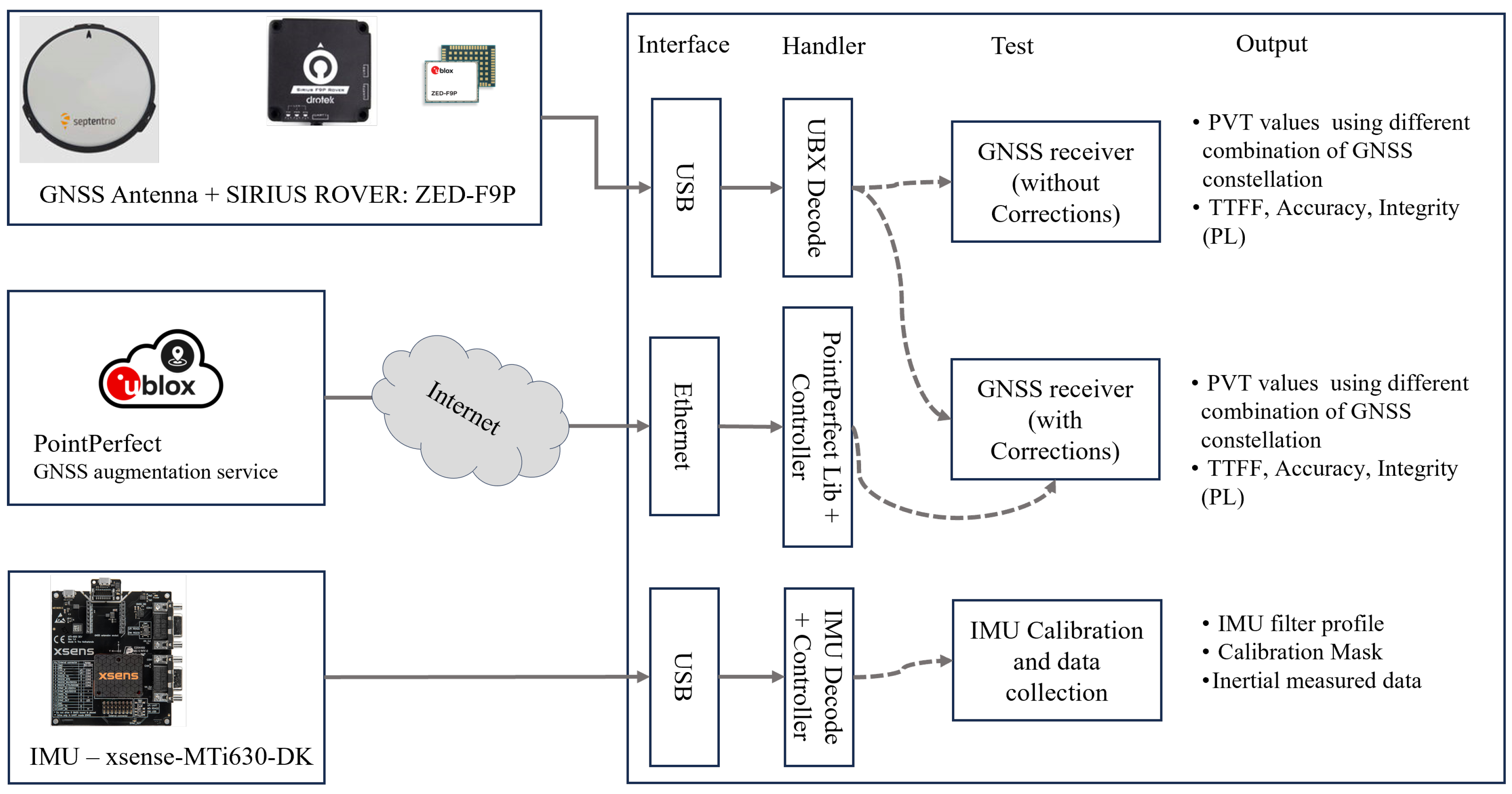
Figure 6 presents a detailed schematic of the experimental verification process conducted for each key system sensor. The purpose of this experimental setup is to evaluate each subsystem and check the individual performances of each sensor. The test also covers the process of interconnection, configuration, decoding, and calibration of the sensors involved. The verification process of the GNSS system (GNSS Antenna + SIRIUS ROVER: ZED-F9P) is a comprehensive series of experimental tests where all the components of the GNSS subsystem are thoroughly evaluated: the antenna, the communication interfaces, the SW block dedicated to decoding, as well as the performances in terms of position calculation (PVT). Furthermore, the impact of the PointPerfect (Augmentation service) is evaluated.
Table 1 shows some performance results that cover the cases of using the GPS and Galileo constellations without PointPerfect service and the case of using the full capability of the GNSS receiver (GNSS + PointPerfect augmentation service). The reference system (known positions) used in the performance calculations was derived from previous long-term PPP-RTK measurements. The inertial measurement system (Xsens—MTi 630 AHRS) is also verified in a stationary scenario. In addition to validating the interfaces, configuration, and SW components dedicated to coding/decoding, this process allows the creation of a data set that was used to characterise the inertial error in the GNSS + IMU integration process.
4.1. Sensors Verification
Before a complete and definitive test of the OBU in a real environment, we present a verification of the performance of some fundamental system elements. Particular interest falls on the satellite navigation system, which includes two fundamental components: the GNSS multi-constellation/multi-frequency receiver and the Augmentation Service, which provides the relevant atmospheric and clock corrections. The sensor verification process allows the performance to be characterised locally through appropriate configuration. For example, it can evaluate satellite availability and coverage (DOP), the average Time To First Fix (TTFF), and the most effective combinations of constellations and frequencies in the case of GNSS.
4.2. Xsens MTi630 AHRS
The tests conducted on the inertial navigation component focused on the calibration process and the correct functionality of the sensor. For this, we used the Xsens Development Kit MTi630 connected to a PC and a SW dedicated to the configuration and storage of data measured by the sensor. The experiment configuration just involves connecting the PC and the MTi-630-DK using the corresponding USB interface. The acquisition SW is implemented in Python and uses the manufacturer open-source API (Xsens Device API) as a library. To summarise the flow followed by the acquisition SW: a first “startup” phase dedicated to the creation of the XDA library objects, scanning of the ports/interfaces and configuration of the device; a second “processing and storage” step dedicated to the manipulation and storage of the inertial data; and finally the step of closing and disconnection of the objects, ports and files used. In addition, a summary of the IMU configuration profile, including motion filters, calibration information and inertial system data, is stored.
4.3. GNSS and Augmentation Service
The whole satellite navigation system testing process is conducted in two steps: one dedicated only to verify the correct functionality of the GNSS receiver, and the other one to evaluate the impact of using the PointPerfect service. For the first step, the HW involved includes the GNSS antenna, the GNSS receiver, and a PC that connects to the receiver via the USB port. In the second step, an Internet connection is needed to access the PointPerfect service. This test is performed in a controlled outdoor environment with the antenna placed on a vehicle at rest.
The tests described in this section focus on the evaluation of the performance of the satellite navigation system, considering the most important parameters in automotive positioning: TTFF, Accuracy, Integrity and satellite availability metrics. The GNSS data acquisition process (with and without corrections) is carried out using an acquisition SW that has the following flow: startup (configuration of interfaces, objects, devices and services); processing (main cycle in charge of decoding the UBX data coming from the GNSS sensor, the corrections coming from the PointPerfect service, and the file storage process); and finally the close and disconnection phase of the elements used. In the case of the TTFF tests, repetitions are performed from a “coldstart” and, afterwards, the mean is applied to the measured values.
4.4. Sensor Integration: On-Road Navigation Test
The integration or fusion process is the core of the multi-sensor approach to navigation. This section describes the verification process applied to the algorithm described in
Section 3. Having characterised the sensors/services in terms of noise, accuracy and response times, the improvements introduced by the integration process can be quantified. In this case we use a Raspberry Pi 4 Model B (On Board Controller), the satellite navigation system described in the previous section (Antenna, Receiver and GNSS Augmentation Service), the MTi630-DK, everything installed within a compact city car.
Figure 7 specifies the coordinate system and reference frame used. In this case, we match the inertial reference frame (i-frame) with the body/vehicle reference frame (b-frame). The conversion process to a unique navigation system (n-frame) uses the corresponding transformations (i.e., Rotation Matrix). Likewise, the reference system used by the ground-referenced GNSS (e-frame) shall be in a compatible reference system to facilitate the fusion process.
The navigation information is captured during the experiment using a data-logger script. The main elements to be stored for future analysis are GNSS information, inertial measurements, timing information, sensor fusion process results, and Kalman filter status information. This experiment has been conducted in the following sequence.
The On-road experiment has been conducted in the parking area of the Tecnopolo of Abruzzo, city of L’Aquila, Italy, and lasted 240 s (4 min). During the test, a trajectory along the marked tracks has been followed, with acceleration intervals and stops, to simulate a typical urban scenario. For this experiment, the inertial sensor samples the data with a frequency of 100 Hz, and the GNSS receives one updated PVT message every second.
5. Results
The most relevant results in evaluating the sensors lie in the accuracy of the satellite navigation system and the improvement obtained using an external GNSS augmentation service. In addition, considering the automotive application, we provide some statistics on the power consumption of the OBU. This section concludes by showing the final results of the sensor fusion application.
5.1. GNSS Performance
The first GNSS key issue analysed was the TTFF measured starting from a “coldstart” signal to the receiver until it reaches a 3D Fix. Experimental results show a mean value slightly below 30 s. This result has been verified and is consistent with the data provided by the manufacturer. However, even if this result is satisfactory, it is important to note that a lower TTFF may be required in automotive applications. This is why the OBU foresees the storage of the last position/status of the vehicle after it has been powered off, functionalities supported thanks to the internally incorporated Power Management and UPS system. The backup battery connected to the Protected 18650 Li-Ion Separable Battery Holder has a capacity of 3000 mAh (at 3.7 V). Assuming OBU consumption in the high operating mode (average power of 5 W and average current of 1 A), the system autonomy, regarding energy, is about 2 h.
Table 1 compiles the results obtained in the evaluation process by accumulating data for more than 5000 s (approximately one and a half hours) at different fixed known positions and times along a given day. The first two columns of the table match the key performance indicators (KPI) with the corresponding measured parameters. Two measurement sets have been collected: one using two GNSS constellations (GPS + GALILEO) without GNSS corrections and the other, including the PointPerfect Augmentation service and using all four GNSS constellations. Measurements collected at different times during multiple trials, are summarized statistically through their mean and variance. Accuracy measures are improved by using the augmentation service, as expected: performance obtained using the GALILEO and GPS constellations simultaneously, but without atmospheric and clock correction, are significantly lower than the ones obtained when the full potential of the GNSS receiver is used. Exploitation of the PointPerfect augmentation service noticeably improves the mean of the accuracy values and also reduces their variance, leading to an improved system’s reliability. Although requirements of the EMERGE reference use cases are satisfied, the recommendation points towards a configuration with a Multi-constellation/multi-frequency approach plus GNSS Augmentation Service. With the perspective to support high and full automated Connected and Automated Driving (CAD) functions, as detailed in 3GPP and ETSI latest specifications [
35], a reduction of the order of magnitude (from metres to centimetres) in the accuracy parameters in the satellite navigation process is more than justified.
One of the advantages of using configurations where all available satellite resources in view are utilised is the ability to select (exclude) the SVs (space vehicles) to be used. This has a direct impact on other satellite navigation KPIs. When using all the potentialities of the receiver, it can be observed doubling of the number of used satellites, as well as an improvement in the Dilution of Precision (DOP) parameters that mitigate the (mathematical) error in the calculation of the position due to the effects of the spatial distribution of the GNSS satellites.
Values of the Integrity, which is a crucial element in automotive applications, may be insufficient for some specific automotive use cases, despite the usage of the GNSS and PointPerfect configuration. This is why other sensors such as Lidar, Radar and Video cameras must be incorporated in specific scenarios and applications. In fact, the EMERGE project foresees the integration of sensors (as external components) in the navigation OBU.
5.1.1. Sensor Integration
This section presents the experimental results obtained using the sensor fusion (SF) algorithm described in
Section 3. To assess the algorithm’s performance under realistic conditions, we conducted tests in an open–sky environment near our laboratory, ensuring clear visibility. We intentionally opted for this setting to maintain flexibility in test conditions and trajectory definition. We decided to focus our tests on real–world scenarios characterized by urban signal degradation, therefore augmenting the GNSS data further would not have provided significant insights. Our aim was to underscore the practical utility of INS in complementing GNSS signals, particularly in scenarios where augmentation may not substantially contribute to improving accuracy or robustness. Hence, we opted to concentrate on the primary GNSS signals from GPS and Galileo, augmented by the INS data. To replicate inaccuracies typically encountered in urban settings, a fault injection operation was applied to the GNSS–only signal (GPS + GALILEO). To simulate the effect of random variations and inaccuracies in the GNSS signal, we employed a Brownian motion process, that generated random additive variations for latitude, longitude, and altitude. In this way, we obtained the estimates of position provided by a degraded GNSS. Subsequently, we evaluated the impact of data fusion in terms of accuracy, stability, and response to errors that affected GNSS without augmentation and IMU sensors.
The tests were conducted near the Abruzzo Technopole, located at Strada Statale 17 Loc. Boschetto di Pile, 67100 L’Aquila (AQ), Italy.
Figure 8,
Figure 9,
Figure 10,
Figure 11 and
Figure 12 illustrate the five test scenarios under consideration. Each figure depicts the starting point of the vehicle detected by each sensor with a circle. The dashed line represents the ground truth, derived from the GNSS signal (all constellations) with PP corrections applied every 5 s. The solid purple line represents the trajectory obtained with GNSS–only, while the solid blue line represents the trajectory obtained from the sensor fusion algorithm, integrating IMU/GNSS data. A preliminary analysis reveals that in each scenario, the trajectory from GNSS–only, which has undergone degradation, deviates further from the ground truth compared to the trajectory returned by the data fusion algorithm.
Figure 13,
Figure 14,
Figure 15,
Figure 16 and
Figure 17 compare, on one side, the graphs of latitude, longitude, and altitude, and on the other side, the error on the same calculated as the distance from the ground truth. The gray line corresponds to GNSS-only, the blue line represents the result of IMU/GNSS integration, and the dashed line represents the ground truth. Here, it becomes even more evident how the algorithm reduces disturbances introduced by GNSS and minimizes error.
This observation is also numerically confirmed in
Table 2 which presents the Root Mean Square Error data calculated with respect to the ground truth for the position obtained with GNSS–only and for the position estimated by the SF algorithm.
These results indicate a substantial discrepancy between the positions estimated via GNSS and the actual positions measured in the field, and demonstrate that the combined use of IMU and GNSS significantly improved the accuracy of position estimation.
The velocity plots in
Figure 18,
Figure 19,
Figure 20,
Figure 21 and
Figure 22 confirm the previous analyses for the same scenarios, with a perfect overlap of the velocity estimates on all three axes for the ground truth, GNSS-only, and the result of data fusion. On the other side, the error on the three axes fluctuates slightly around zero, confirming the algorithm’s good performance.
6. Conclusions
This paper presents the OBU architecture for the EMERGE project, and the implementation of the navigation system, based on a multi–sensor approach.
The proposal of a concrete architecture for OBU development provides a starting point in the automotive field for other application areas and services. Although in the test–bed used for this work most of the processing has been performed locally, the presented architecture can be applied to systems that foresee a microservice approach, cloud computing [
36], and/or edge computing. This transformation entails moving some elements (mainly from the core layer of the onboard system architecture, i.e., layer 4 in
Figure 1) out of the OBU and enhancing elements dedicated to communication, according to specific performance requirements. The modular architecture has helped in using the agile methodology for developing the product, facilitating the selection process of HW components and technologies, and error debugging.
Experimental tests conducted on inertial and GNSS sensors have demonstrated their accuracy, that satisfies performance requirements of the EMERGE project and justifies their use in real automotive scenarios. The GNSS receiver provides excellent performance when integrated with the u–blox augmentation system, i.e., PointPerfect, that enhances the accuracy of the satellite navigation system from metres to centimetres. This work uses the u–blox commercial IP plan, which provides corrections through an MQTT broker. The subscription to the root topic provides to the experiment all the set of corrections—i.e., orbits, bias, atmosphere, and clock—whenever they are available. The effectiveness of the multi–sensor approach has also been validated in challenging scenarios like urban contexts. In fact, tests documented in
Section 5.1.1 show that merging inertial and satellite data provides a more accurate estimate of the trajectory, particularly when the GNSS is degraded.
Implementing an OBU in the automotive context also involves the power analysis of the system. The Power Management and UPS systems guarantee the operating autonomy needed by the OBU to conclude and store the states of the active processes.
Author Contributions
Conceptualisation, all authors; methodology, all authors; software, A.L.Z.S., V.I., M.B. and M.P.; validation, A.L.Z.S., V.I., M.P., M.B., F.V. and E.C.; formal analysis, all authors; investigation, all authors; resources, all authors; data curation, A.L.Z.S., V.I., M.P., M.B., F.V. and E.C.; writing—original draft preparation, A.L.Z.S., V.I., M.P., F.V. and E.C.; writing—review and editing, A.L.Z.S., V.I., M.P., M.B., F.V. and E.C.; visualisation, all authors; supervision, M.P., R.A., F.V., E.C., C.A. and A.M.; project administration, F.V. and M.P.; funding acquisition, all authors. All authors have read and agreed to the published version of the manuscript.
Funding
This research was partly funded by the project “Centre of Excellence on Connected, Geo–Localized and Cyber–secure Vehicles”–Italian Government (Grant Number: CIPE Resolution 70/2017) and the project EMERGE–Navigation (Ministry of Innovation and Made in Italy and Regione Abruzzo).
Institutional Review Board Statement
Not applicable.
Informed Consent Statement
Not applicable.
Data Availability Statement
The data that support the findings of this study are available from the corresponding authors, A.Z. and V.I., upon reasonable request.
Acknowledgments
The authors acknowledge the Ex-EMERGE centre, Radiolabs and Telespazio Spa for the support, resources and facilities provided. Special thanks to Graziano Battisti/DISIM-UNIVAQ for his invaluable technical assistance during this research. Their expertise and support have played a crucial role in successfully executing this work.
Conflicts of Interest
The authors declare no conflict of interest.
Abbreviations
The following abbreviations are used in this manuscript:
| ADAS | Advanced Driver Assistance System |
| AGNSS | Augmented GNSS |
| AHRS | Attitude and Heading Reference Systems |
| API | Application programming interface |
| AV | Autonomous Vehicle |
| C/N0 | Carrier-to-Noise Density Ratio |
| CAD | Connected and Automated Driving |
| COTS | Commercial Off-The-Shelf |
| DOP | Dilution Of Precision |
| ECEF | Earth-centred, Earth-fixed Coordinate System |
| EKF | Extended Kalman Filter |
| GNSS | Global Navigation Satellite System |
| GPIO | General Purpose Input/Output |
| GT | Ground Truth |
| HW | Hardware |
| IMU | Inertial Measurement Unit |
| INS | Inertial Navigation System |
| IoT | Internet of Things |
| IP | Internet Protocol |
| JSON | JavaScript Object Notation |
| KPI | Key Performance Indicators |
| MCU | Microcontroller Unit |
| MQTT | Message Queuing Telemetry Transport |
| MT | Motion Trackers |
| NED | North-East-Down |
| OBC | On Board Computer |
| OBU | On Board Unit |
| PNT | Positioning, Navigation and Timing |
| PP | PointPerfect |
| PPP | Precise Point Positioning |
| PPP-RTK | Precise Point Positioning - Real Time Kinematic |
| PVT | Position, Velocity and Time |
| RMSE | Root Mean Square Error |
| RTK | Real Time Kinematic |
| SBC | Single Board Computer |
| SDRAM | Synchronous Dynamic Random Access Memory |
| SF | Sensor Fusion |
| SMA | SubMiniature version A - coaxial RF connector |
| SoC | System-on-a-Chip |
| SVs | Space Vehicles |
| SW | Software |
| TTFF | Time To First Fix |
| UAV | Unmanned Aerial Vehicle |
| UBX | u-blox proprietary binary protocol |
| UPS | Uninterruptible Power Supply |
| V2V | Vehicle to Vehicle communications |
| V2X | Vehicle to Everything communications |
| XDA | Xsens Device API |
Appendix A. Extended Kalman Filter (NED Implementation)
In this appendix, the expressions for the matrices used in the Kalman filter prediction and correction steps when attitude and velocity are Earth-referenced and resolved in the local (NED) navigation frame, and the position is expressed using geodetic coordinates, are reported. The index denoting the epoch is omitted in the equations for readability. However, it should be understood that all equations are formulated explicitly for a specific epoch k.
State prediction matrix:
where
Prediction error covariance matrix:
where
,
,
, and
denote, respectively, the power spectral densities of the noise of the gyroscope and accelerometer, and the power spectral densities of the bias variations of the gyroscope and accelerometer.
Vector of observations:
is given by the difference between the position and velocity solution of the GNSS and the corrected inertial navigation solution, plus a term to account for the displacement between the inertial platform and the GNSS antenna,
.
References
- United Nations: Department of Economic and Social Affairs Population Dynamics. World Urbanisation Prospects 2018—Processed by Our World in Data. “Urban”. Available online: https://population.un.org/wup/Download/ (accessed on 12 September 2023).
- Faria, R.; Brito, L.; Baras, K.; Silva, J. Smart mobility: A survey. In Proceedings of the 2017 International Conference on Internet of Things for the Global Community (IoTGC), Funchal, Portugal, 10–13 July 2017; pp. 1–8. [Google Scholar] [CrossRef]
- Paiva, S.; Ahad, M.; Tripathi, G.; Feroz, N.; Casalino, G. Enabling technologies for urban smart mobility: Recent trends, opportunities and challenges. Sensors 2021, 21, 2143. [Google Scholar] [CrossRef] [PubMed]
- Ribeiro, P.; Dias, G.; Pereira, P. Transport systems and mobility for smart cities. Appl. Syst. Innov. 2021, 4, 61. [Google Scholar] [CrossRef]
- Xiang, C.; Feng, C.; Xie, X.; Shi, B.; Lu, H.; Lv, Y.; Yang, M.; Niu, Z. Multi-Sensor Fusion and Cooperative Perception for Autonomous Driving: A Review. IEEE Intell. Transp. Syst. Mag. 2023, 15, 36–58. [Google Scholar] [CrossRef]
- Yeong, D.; Velasco-Hernandez, G.; Barry, J.; Walsh, J. Sensor and sensor fusion technology in autonomous vehicles: A review. Sensors 2021, 21, 2140. [Google Scholar] [CrossRef]
- Mailka, H.; Abouzahir, M.; Ramzi, M. An efficient end-to-end EKF-SLAM architecture based on LiDAR, GNSS, and IMU data sensor fusion for autonomous ground vehicles. Multimed. Tools Appl. 2023, 83, 56183–56206. [Google Scholar] [CrossRef]
- Santa, J.; Bernal-Escobedo, L.; Sanchez-Iborra, R. On-board unit to connect personal mobility vehicles to the IoT. In Proceedings of the 17th International Conference on Mobile Systems and Pervasive Computing (MobiSPC), Leuven, Belgium, 9–12 August 2020; Volume 175, pp. 173–180, ISSN 18770509. [Google Scholar] [CrossRef]
- Ganeshkumar, N.; Kumar, S. OBU (On-Board Unit) Wireless Devices in VANET(s) for Effective Communication—A Review. In Computational Methods and Data Engineering. Advances in Intelligent Systems and Computing; Singh, V., Asari, V.K., Kumar, S., Patel, R.B., Eds.; Springer: Singapore, 2021; Volume 1257. [Google Scholar] [CrossRef]
- He, L.; Deng, Z.; Huang, J. Navigation and communication platform for on board unit of logistics traffic. In Proceedings of the 2009 Joint Conferences On Pervasive Computing (JCPC), Tamsui, Taiwan, 3–5 December 2009; pp. 305–308. [Google Scholar] [CrossRef]
- Schindler, N. On Board Unit for the European Electronic Tolling Service. In Proceedings of the 9th ITS European Congress, Dublin, Ireland, 4–7 June 2013; ERTICO (ITS Europe). Available online: https://www.gnss-consulting.com/wp-content/uploads/2018/12/2013-Schindler-OBU-for-the-European-Electronic-Tolling-Service-Hybrid-Electronic-Tolling-Solution-9thITS-Dublin.pdf (accessed on 6 June 2023).
- Santa, J.; Skarmeta, A.; Ubeda, B. An Embedded Service Platform for the Vehicle Domain. In Proceedings of the 2007 IEEE International Conference on Portable Information Devices, Orlando, FL, USA, 25–29 May 2007; pp. 1–5. [Google Scholar] [CrossRef]
- Noureldin, A.; Karamat, T.B.; Georgy, J. Fundamentals of Inertial Navigation. In Satellite-Based Positioning and Their Integration; Springer: Berlin/Heidelberg, Germany, 2013; Volume 1, p. 313. [Google Scholar]
- Tamazin, M.; Karaim, M.; Noureldin, A. GNSSs, Signals, and Receivers. In Multifunctional Operation and Application of GPS; Rustamov, R.B., Hashimov, A.M., Eds.; IntechOpen: Rijeka, Croatia, 2018; Chapter 6; pp. 69–85. [Google Scholar]
- Zhu, N.; Marais, J.; Bétaille, D.; Berbineau, M. GNSS Position Integrity in Urban Environments: A Review of Literature. IEEE Trans. Intell. Transp. Syst. 2018, 19, 2762–2778. [Google Scholar] [CrossRef]
- Reid, T.G.R.; Houts, S.E.; Cammarata, R.; Mills, G.; Agarwal, S.; Vora, A.; Pandey, G. Localization Requirements for Autonomous Vehicles. SAE Intl. J CAV 2019, 2, 173–190. [Google Scholar] [CrossRef]
- Groves, P.D. Principles of GNSS, Inertial, and Multisensor Integrated Navigation Systems; Artech House: Boston, MA, USA, 2013; Chapter 14; pp. 559–589. [Google Scholar]
- Overview of the EMERGE Initiative: Connected, Geo-Localized and Cybersecure Vehicles. Available online: http://exemerge.disim.univaq.it/?page_id=342 (accessed on 11 December 2023).
- Di Sciullo, G.; Zitella, L.; Cinque, E.; Santucci, F.; Pratesi, M.; Valentini, F. Experimental Validation of C-V2X Mode 4 Sidelink PC5 Interface for Vehicular Communications. In Proceedings of the 2022 61st FITCE International Congress Future Telecommunications: Infrastructure and Sustainability (FITCE), Rome, Italy, 29–30 September 2022; pp. 1–6. [Google Scholar] [CrossRef]
- Tiberti, W.; Civino, R.; Gavioli, N.; Pugliese, M.; Santucci, F. A Hybrid-Cryptography Engine for Securing Intra-Vehicle Communications. Appl. Sci. 2023, 13, 13024. [Google Scholar] [CrossRef]
- u-blox. ZED-F9P High Precision GNSS Module Integration Manual. 30 August 2023. Available online: https://content.u-blox.com/sites/default/files/ZED-F9P_IntegrationManual_UBX-18010802.pdf (accessed on 6 September 2023).
- u-blox. PointPerfect Product Summary. 2021. Available online: https://content.u-blox.com/sites/default/files/PointPerfect_ProductSummary_UBX-21024758.pdf (accessed on 11 June 2023).
- u-blox. u-blox Services Product Overview: IoT Location-as-a-Service. 2023. Available online: https://content.u-blox.com/sites/default/files/SER-product_Overview_UBX-21029993.pdf (accessed on 10 November 2023).
- Movella. MTi-630 AHRS Datasheet. May 2023. Available online: https://www.xsens.com/hubfs/Downloads/Leaflets/MTi-630.pdf (accessed on 10 November 2023).
- Movella. MTi 600-Series Datasheet: IMU, VRU, AHRS and GNSS/INS. June 2023. Available online: https://www.xsens.com/hubfs/Downloads/Leaflets/MTi%20600-series%20Datasheet.pdf (accessed on 10 November 2023).
- MQTT Version 5.0 OASIS Standard. 7 March 2019. Available online: https://docs.oasis-open.org/mqtt/mqtt/v5.0/mqtt-v5.0.pdf (accessed on 10 November 2023).
- Sixfab. Sixfab Raspberry Pi 3G-4G/LTE Base HAT Datasheet: V1.0. 2019. Available online: https://sixfab.com/wp-content/uploads/2020/03/Sixfab_3G-4G-LTE_Base_HAT_Datasheet_V1.0.pdf (accessed on 22 May 2023).
- Sixfab. Sixfab API Documentation. Available online: https://sixfab.github.io/sixfab-power-python-api/ (accessed on 9 September 2023).
- Node-RED: Low-Code Programming for Event-Driven. Node-RED Documentation. Available online: https://nodered.org/docs/ (accessed on 14 September 2023).
- Raspberry Pi (Trading) Ltd. Raspberry Pi 4 Model B DATASHEET: Release 1. June 2019. Available online: https://datasheets.raspberrypi.com/rpi4/raspberry-pi-4-datasheet.pdf (accessed on 12 February 2023).
- Drotek. Sirius RTK GNSS Rover (F9P): Compact; High-Precision L1/L2 GNSS Rover Based on U-blox ZED-F9P (GPS/GLONASS/BeiDou/Galileo). March 2020. Available online: https://static1.squarespace.com/static/5619914ce4b07e497b442de9/t/5f29cc9638612318c900f5c1/1596574874260/DrotekDoc_0911A+-+Sirius+RTK+GNSS+Rover+%28F9P%29.pdf (accessed on 22 June 2023).
- El-Sheimy, N.; Hou, H.; Niu, X. Analysis and Modeling of Inertial Sensors Using Allan Variance. IEEE Trans. Instrum. Meas. 2008, 57, 140–149. [Google Scholar] [CrossRef]
- Groves, P.D. Principles of GNSS, Inertial, and Multisensor Integrated Navigation Systems; Artech House: Boston, MA, USA, 2013; Chapter 5; pp. 163–187. [Google Scholar]
- Groves, P.D. Principles of GNSS, Inertial, and Multisensor Integrated Navigation Systems; Artech House: Boston, MA, USA, 2013; Chapter 15; pp. 638–641. [Google Scholar]
- ETSI TS 122 186 V17.0.0. 5G; Service Requirements for Enhanced V2X Scenarios (3GPP TS 22.186 Version 17.0.0 Release 17). (2022-04). Available online: https://www.etsi.org/deliver/etsi_ts/122100_122199/122186/17.00.00_60/ts_122186v170000p.pdf (accessed on 10 September 2023).
- Desirena Lopez, H.; Siller, M.; Huerta, I. Internet of vehicles: Cloud and fog computing approaches. In Proceedings of the 2017 IEEE International Conference on Service Operations and Logistics, and Informatics (SOLI), Bari, Italy, 18–20 September 2017; pp. 211–216. [Google Scholar] [CrossRef]
| Disclaimer/Publisher’s Note: The statements, opinions and data contained in all publications are solely those of the individual author(s) and contributor(s) and not of MDPI and/or the editor(s). MDPI and/or the editor(s) disclaim responsibility for any injury to people or property resulting from any ideas, methods, instructions or products referred to in the content. |
© 2024 by the authors. Licensee MDPI, Basel, Switzerland. This article is an open access article distributed under the terms and conditions of the Creative Commons Attribution (CC BY) license (https://creativecommons.org/licenses/by/4.0/).


 ,
, 


