Study on Classification of Fishing Vessel Operation Types Based on Dilated CNN-IndRNN

Abstract

At present, fishery resources are becoming increasingly depleted, and a reliable assessment of fishing activity is a key step in protecting marine resources. Correctly identifying the type of fishing operation can help identify illegal fishing vessels, strengthen fishing regulations, and prevent overfishing. Aiming to address these problems, this study first collects and preprocesses fishing vessel AIS data. Improvements are proposed on the basis of the convolutional neural network (CNN), long short-term memory (LSTM), and other models, changing the CNN to dilated CNN and LSTM to independently recurrent neural network (IndRNN). The results of the experiment show that the accuracy, precision, recall, and F-1 score of the model are finally obtained as 93.12%, 93.10%, 93.14%, and 93.10%, respectively. Overall, the new model proposed in this study offers a significant improvement in performance compared to the models of other scholars in the past.

1. Introduction

Nowadays, the increasing exploitation of global resources and the rapid growth of the population have resulted in resource shortages, environmental pollution, and many other problems [1]. Based on this situation, people are gradually shifting their horizons from inland to the oceans in the hope of obtaining additional resources [2]. With the continuous development of shipbuilding technology, the number of fishing vessels in the world has increased, and fishing vessels are gradually evolving into large and high-speed vessels. Different types of fishing vessels have different fishing ranges and cause different levels of damage to fishery resources [3,4,5]. Categorizing and identifying the types of fishing vessel operations can strengthen the protection of fishery resources and combat illegal fishing. For example, a fishing vessel that exceeds its operating range, fishes in the wrong sea area, or fishes at a time when fishing is prohibited, can be judged as illegal fishing [6,7,8].

Identifying the type of operation of fishing vessels has always been the focus of fishery administration. With the development of the modernization of fishing vessels, the Global Positioning System (GPS) and Beidou systems have been put into use one after another, laying a solid foundation for a large amount of data collection. At present, the most widely used vessel monitoring system (VMS) is the Automatic Identification System (AIS), which is designed to ensure the safety of vessel navigation [9,10,11]. There are great differences in the operation trajectories of different vessels, which can be recognized according to the AIS data [12,13,14].

Kroodsma et al. [15] processed 22 billion worldwide AIS data from 2012 to 2016. They trained two convolutional neural networks, one to identify the type of fishing vessel operation and the other to detect the fishing status. The model was able to identify six types of fishing vessels and six types of non-fishing vessels. The accuracy of identifying the types of fishing vessels was up to 95%, and the accuracy of identifying the fishing status was up to 90%. This study collected sufficiently rich data to ensure that the model is trained to achieve a high accuracy rate, but there is still room for optimization in the model structure. Kim et al. [16] identified six fishing gear types based on vessel AIS data and environmental data using a deep learning-based approach for gear type recognition. To capture the complex dynamic patterns in the trajectories of gear types, a sliding window-based data-slicing method was used to generate the training dataset. In order to compare the performance of the proposed models, a support vector machine (SVM) model was also developed. The CNN model showed an average of 0.963 dots per inch (DPI), while the SVM model showed an average of 0.814 DPI. The results show that the model can effectively identify the gear types of the fishing vessels. Storm et al. [17] proposed a vessel geospatial trajectory analysis visualization system (VA-TRAC), which accomplished the monitoring, identification, and verification of fishing vessel trajectories, aiming to solve the problem of illegal fishing. This work provides an effective identification of illegal fishing behavior by fishing vessels, which is of great significance in the regulation of fishing vessels. Park [18] grouped speed and heading time series and constructed six offshore fishing vessel category identification models for the Korean Peninsula using the image recognition method. Finally, Ericon N. et al. [19] used different models for different types of fishing vessels, including a hidden Markov model for trawlers, with the observed variable being vessel speed, which ultimately achieved 83% accuracy.

The above studies generally used the model of a convolutional neural network, which is slightly simpler in model structure and lacks the ability to extract features from complex fishing vessel AIS sequence data. In this paper, a deep learning model combining the dilated CNN and IndRNN was used to improve the feature extraction ability of the model and obtain better recognition results.

2. Methods

2.1. Data Preparation

This study is based on the fishing vessel AIS data from the Ali Tianchi competition (https://tianchi.aliyun.com/dataset/, accessed on 25 September 2023), which contains the trajectory information of more than 18,329 fishing vessels, among which there are 6189 trawlers, 6099 purse seiners, and 6041 gillnets, and each trajectory information contains the six basic elements of longitude, latitude, speed, heading, time, and type of fishing operation.

2.2. Data Preprocessing

Preprocessing for AIS data is mainly reflected in the treatment of missing values and outliers. Missing values need to be completed by interpolation according to the before and after data. Outliers should be recognized first and then completed by interpolation after deleting.

Currently, AIS technology is not yet fully matured, resulting in a partial absence of ship track trajectory points; therefore, some processing of the missing data is needed. Figure 1 shows the missing trajectory data map; the blue points indicate the actual data that have been recorded, and the black points indicate the missing data to compensate for the missing data values [20]. The numbers are markers for the points.

Since the trajectory data is a column of time series, the location where the missing values need to be interpolated can be determined based on the time interval between two neighboring data points, and the number of missing points is directly proportional to the time interval. The larger the time interval between two neighboring data points, the greater the number of missing points.

To identify missing values, we used the method of judging the time interval to identify missing values, with a time interval of 10 min. Let the time series of the original AIS data be $T=\{t_1,t_2,\dots ,t_n\}$, and calculate the time interval between any two adjacent time points $\Delta t=t_j-t_k$, when $\Delta t<20$, which does not need to be supplemented. When $20\le \Delta t<30$, it needs to supplement one point. When $30\le \Delta t<40$, it needs to supplement two points, and so on. In the filling in of missing values, the data were supplemented using Lagrange interpolation.

A polynomial passing through all known points can be obtained by Lagrange interpolation. Based on the existing trajectory of the fishing boat, all known points can be brought in to obtain the polynomial, and then the value at the missing place can be calculated from the polynomial, as shown in the following formula [21].

$$P_n(t)={\displaystyle \sum _{i=1}^n{k}_{t_i}({\displaystyle \prod _{j\ne i}^{1\le j\le n}\frac{(t-t_j)}{(t_i-t_j)}}})$$

(1)

Due to the different configuration of fishing vessel facilities for different types of operations, the range of speed and heading range that can be reached is also different, and there is no clear regulation. AIS data of fishing boats record the instantaneous speed and instantaneous course of fishing boats, which are easily affected by waves, strong winds, and other factors, and are prone to noise values. Therefore, it is necessary to process the abnormal value of the collected AIS data to avoid adverse effects on the subsequent model training.

Let D be the difference between the current velocity value and the previous velocity value, and F be the velocity threshold. When D > F, the distance l between the current data point and the previous data point is calculated by the current velocity. The distance l is compared with the actual distance d between the two data points calculated by the Haversine formula. If the distance l is close to the actual distance d, it is considered that the current velocity value is normal. On the contrary, it is considered that the current velocity value is abnormal, and the data value needs to be corrected. The Harversine formula is:

$$d=2r{\sin }^{-1}\left(\sqrt{{\sin }^2\left(\frac{{\varphi }_2-{\varphi }_1}{2}\right)+\cos \left({\varphi }_1\right)\cos \left({\varphi }_2\right){\sin }^2\left(\frac{{\psi }_2-{\psi }_1}{2}\right)}\right)$$

(2)

where, d represents the actual distance between the two points and r represents the radius of the earth, generally selected as 6,378,137 m. $\left({\psi }_1,{\varphi }_1\right)$,$\left({\psi }_2,{\varphi }_2\right)$ represents the latitude and longitude of the previous data point and the latter data point, respectively.

The latitude and longitude anomaly refers to the non-normal deviation of the trajectory point in a small time, which will adversely affect the judgment of the subsequent model. It is necessary to delete the data point and perform an interpolation-filling calculation. According to the degree of variation before and after the trajectory point, we can judge whether there is a deviation problem in the trajectory point. Suppose that the current trajectory point is $T_i$, the previous data point is $T_{i-1}$, the latter data point is $T_{i+1}$, the midpoint of $T_{i-1}$ and $T_{i+1}$ is $T_m$, $d_1$ represents the distance between $T_m$ and $T_i$, and $d_2$ represents the distance between $T_{i-1}$ and $T_{i+1}$. When $d_1>d_2$, the current data point can be considered as a latitude and longitude anomaly point. The anomaly point can be deleted first, and then the interpolation method introduced above is used to fill the data.

Sequence slicing is a data preprocessing technique that involves dividing a long sequence into a series of shorter subsequences, which is widely used in time series analysis. Its main functions include managing long sequences and alleviating computer memory limitations. By fixing the length input, sequences of different lengths are transformed into consistent shapes to adapt to the deep learning model. When dealing with data such as text or time series, slicing can help the model capture short-term time dependencies, which helps reduce the computational complexity and may improve model performance. Due to the huge difference in the number of trajectory points of each fishing vessel in the AIS dataset used in this paper, the sequence slicing method proposed in this paper is to divide the trajectory data of different lengths into statistical segments with a unified number of segments.

The state vector of the fishing vessel at time t can be represented by ${\overrightarrow{X}}_t$. It contains four state values, the latitude (lat), longitude (lon), speed, and heading direction of the ship at time t, as shown in Formula (3).

$${\overrightarrow{X}}_t=(\mathrm{lat},\mathrm{lon},\mathrm{speed},\mathrm{directional})$$

(3)

Then all the state vectors experienced by a fishing boat from time 0 to time H can form the original data matrix A of the whole fishing boat.

$$A={({\overrightarrow{X}}_0,{\overrightarrow{X}}_1,\dots ,{\overrightarrow{X}}_H)}^T$$

(4)

We use L to represent the total length of a trajectory and divide it into N segments on average; then the time step of each segment is T. $T=\frac{L}{N}$; then the new data matrix X_segment is:

$$X\_segment=\left[\begin{array}{cccc}{\overrightarrow{X}}_0,& {\overrightarrow{X}}_1,& \dots & {\overrightarrow{X}}_{T-1}\\ {\overrightarrow{X}}_T,& {\overrightarrow{X}}_{T+1},& \dots & {\overrightarrow{X}}_{2T-1}\\ \dots & \dots & \dots & \dots \\ {\overrightarrow{X}}_{NT},& {\overrightarrow{X}}_{NT+1}& \dots & {\overrightarrow{X}}_{NT+T-1}\end{array}\right]$$

(5)

The speed, course, latitude, and longitude of the fishing vessel can be used as the characteristics to judge the type of fishing vessel operation. According to the slice results, the characteristics of each section are extracted. The maximum, minimum, average, median, and standard deviation of different characteristics are counted below. Its feature matrix is X_feature.

$$X\_feature=\left[\begin{array}{cccc}{F}_{1,1}& F_{1,2}& \dots & F_{1,20}\\ F_{2,1}& F_{2,2}& \dots & F_{2,20}\\ \dots & \dots & \dots & \dots \\ F_{64,1}& F_{64,2}& \dots & F_{64,20}\end{array}\right]$$

(6)

3. Model Building

3.1. Dilated CNN

In the CNN, each convolutional layer consists of a set of convolutional kernels through which the features of the image are extracted [22]. In this process, each element of each output feature map corresponds to a region on the input feature map, as shown in Figure 2. Where 5 × 5 matrix is the target image and numbers are the features. 3 × 3 matrix is the convolution kernel.

The convolution kernel slides on the input data. At each position, the convolution kernel is multiplied by a local area of the input data element by element, and the results of all the products are summed. The result of the summation is taken as the value of the corresponding position in the output feature map. Repeat the above steps until the complete input data are traversed to generate a complete output feature map. The choice of convolution kernel is very important, as it determines the filtering method. Different convolution kernels will obtain different features. The specific formula of the convolution operation is:

$$C(x,y)={\displaystyle \sum _{i=1}^m{\displaystyle \sum _{j=1}^n(X(x+i-1,y+j-1)\cdot K(i,j))+b}}$$

(7)

$C(x,y)$ represents the value of the output feature map at position $(x,y)$, X represents the input feature map, K represents the convolution kernel, m and n represent the size of the convolution kernel, and b is the bias.

A limit of convolutional layers is that they greatly increase the number of parameters in the output tensors compared to the input ones, especially when many filters are involved, then the magnitude of the tensors grows exponentially. For this reason, a pooling layer usually succeeds a convolutional one. Its purpose is to sub-sample the feature map by retaining only the most attractive information extracted by the convolutional layer. There are many possible pooling functions, but in this work, the MaxPooling one is adopted, which takes only the max value out of a predefined sub-matrix [23].

A fully connected layer is a common layer type in convolutional neural networks. A fully connected layer is generally used as the last few layers of the CNN model, which is used to compress and transform the features extracted from the convolutional layer and the pooling layer, and finally map the features to the output category. In the fully connected layer, each neuron is connected to all neurons in the previous layer, and each connection has a corresponding weight parameter to adjust the weight of the input signal.

The receptive field is the size of the region on the input image corresponding to each output feature map element in a convolutional neural network. It represents the perceptual range of each location in the network, i.e., the size of the input image region used to compute the output features. The size of the sensory field depends on several factors:

(1)

Convolution kernel size. Receptive field controlled by convolutional kernel size. Larger convolution kernels can capture more contextual information, but they also increase the amount of computation and the number of parameters.

(2)

The number of convolutional layers. The perceptual field of each output feature map increases as the depth of the network increases because the output feature map of each convolutional layer is a summary of a certain region on the input feature map of the previous layer.

(3)

Step size and pooling operation. The step size is the distance the convolution kernel slides over the input feature map, and the pooling operation downsamples the input feature map. Larger step sizes and pooling operations reduce the size of the sensory field because each output feature map element is associated with only a portion of the input feature map [24,25].

The size of the receptive field is important for feature extraction. A smaller receptive field may not be able to capture large-scale features in an image, while a larger receptive field can provide more global contextual information. Therefore, this chapter adds dilated convolution. It expands the receptive field by introducing dilated means in the convolution kernel, thus increasing the perceptual range of the network and improving the model’s ability to perceive large-scale features. In the traditional convolution operation, the convolution kernel slides over the input feature map in fixed steps and performs the convolution operation at each position. Dilated convolution, on the other hand, is performed by introducing a fixed interval between the elements of the convolution kernel, which can be an arbitrary positive integer, usually denoted by the dilated rate. This increases the range of features that can be acquired. The scheme is presented in Figure 3 below, and the formula is shown in 8 below.

$$Y_{ij}={\displaystyle \sum _m{\displaystyle \sum _n{X}_{i\cdot r+m\cdot d,j\cdot r+n\cdot d}\cdot W_{mn}}}$$

(8)

where $Y_{ij}$ denotes the value at position $(i,j)$ in the output feature map, $X_{i\cdot r+m\cdot d,j\cdot r+n\cdot d}$ denotes the value at position $(i\cdot r+m\cdot d,j\cdot r+n\cdot d)$ in the input feature map, r is the step size of the convolution, $W_{mn}$ denotes the weight value at position $(m,n)$ in the convolution kernel, and d denotes the dilation rate.

Compared with traditional methods, dilated convolution has several advantages. (1) Increasing the receptive field: Increase the receptive field to obtain more feature information. This is useful for dealing with large-scale features or scene understanding tasks. (2) Reducing the number of parameters: While keeping the range of the sensory field constant, dilation convolution can use a smaller convolution kernel size, which reduces the parameter. This helps reduce the computational burden on the model and improves operational efficiency. (3) Maintaining feature map resolution: Ordinary convolution operations will continuously reduce the resolution of the feature map as the number of layers increases. Dilated convolution can maintain the resolution of the feature map by increasing the dilated rate, thus avoiding the loss of information.

Since the data processed in this paper are one-dimensional sequence data, the two-dimensional dilated convolution is improved to one-dimensional dilated convolution. The schematic diagram of one-dimensional inflationary convolution is shown in Figure 4. Similar to two-dimensional inflationary convolution, the one-dimensional inflationary convolution expands the sensory field by introducing the dilated rate, thus increasing the network’s ability to perceive the contextual information of the sequence data. The specific formula is:

$$Y_i={\displaystyle \sum _m{X}_{i\cdot r+m\cdot d}\cdot W_m}$$

(9)

Where $Y_i$ denotes the value of the i element of the output sequence Y, and $X_{i\cdot r+m\cdot d}$ denotes the value of the element in the input sequence X, where r is the step size of the convolution, d is the dilation rate, and $W_m$ denotes the value of the weight at m in the dilated convolution kernel.

One-dimensional inflated convolution has several advantages when dealing with one-dimensional sequential data [26]:

(1)

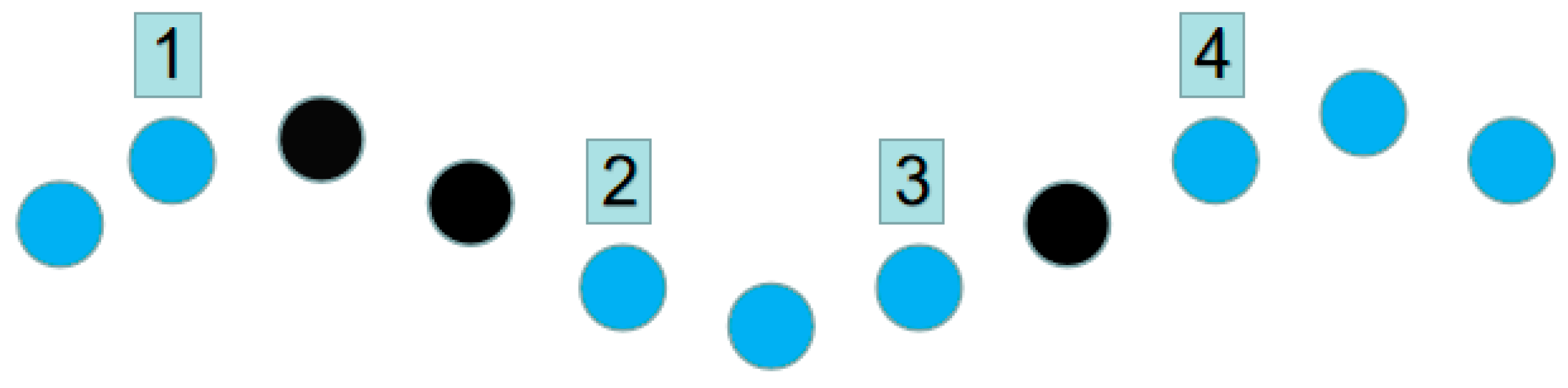
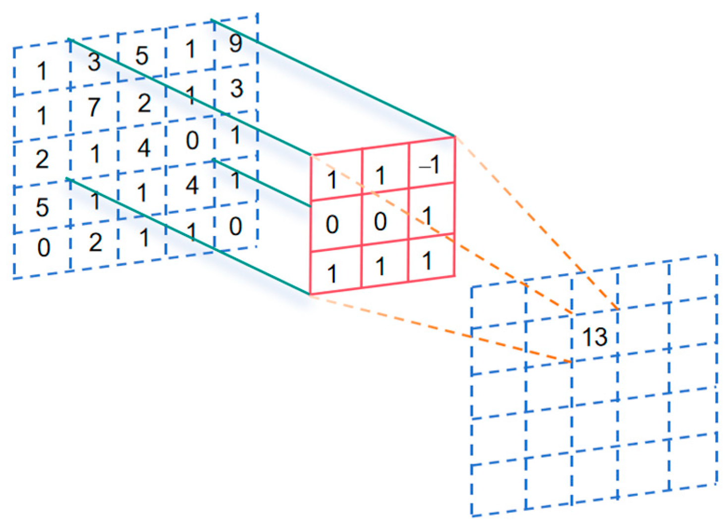
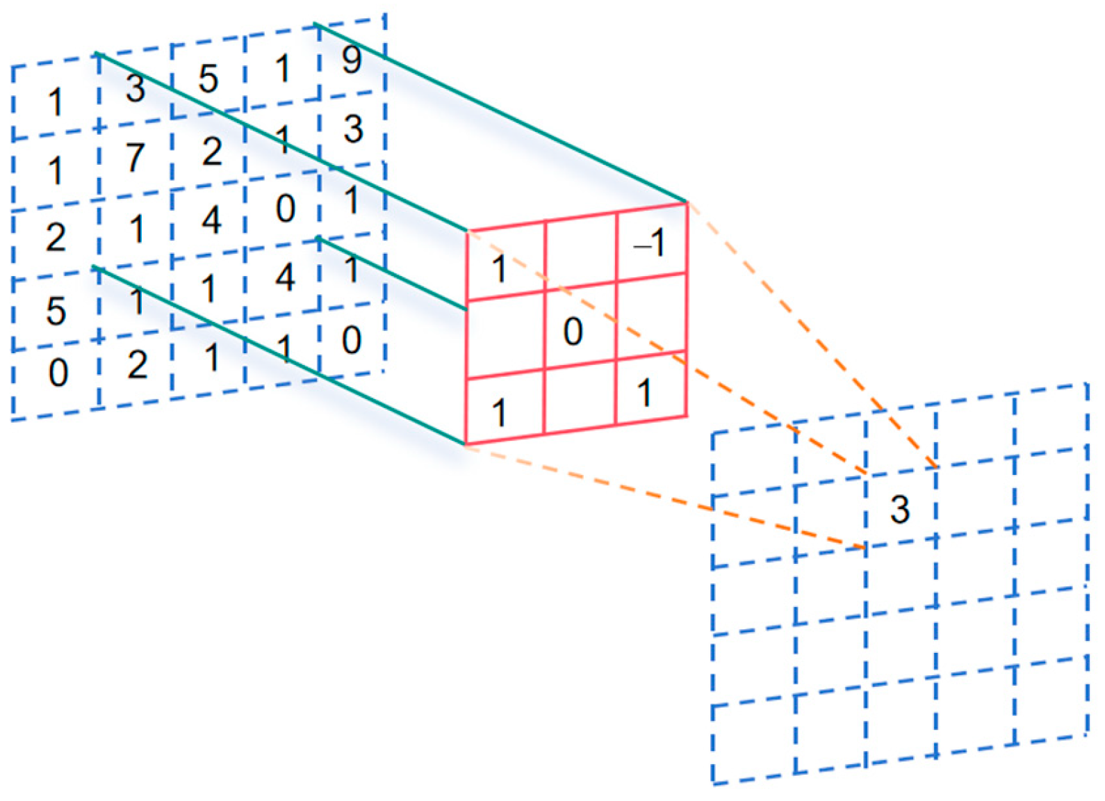
Expanding the sensory field. One-dimensional inflated convolution expands the sensory field by adjusting the dilated rate. A larger dilated rate increases the range of observation of the input sequence by the convolution kernel, thus providing broader contextual information. This is useful for capturing long-term dependencies and understanding associations at long distances in the sequence.

(2)

Reduced number of parameters. Compared to traditional one-dimensional convolution, one-dimensional inflated convolution can use a smaller convolution kernel size to achieve the same range of sensory fields. By introducing the dilated rate, the number of parameters in the model can be effectively reduced, reducing the computational burden of the model and improving its efficiency.

(3)

Maintaining sequence length. In the traditional one-dimensional convolution, the convolution operation causes the length of the output sequence to shrink. And one-dimensional dilated convolution can keep the length of the input sequence and the output sequence the same by adjusting the dilated rate, which avoids the loss of information. Multi-scale feature extraction is possible; by applying one-dimensional dilated convolution at different levels and different dilated rates, features at multiple scales can be extracted at the same time. This helps to capture patterns and correlations on different time scales in sequence data and enhances the expressive power of the model.

Sequence processing capability. One-dimensional inflationary convolution has a strong processing capability when dealing with sequence data; it can effectively capture local patterns and global dependencies in sequences, which is very effective for the processing of one-dimensional signals.

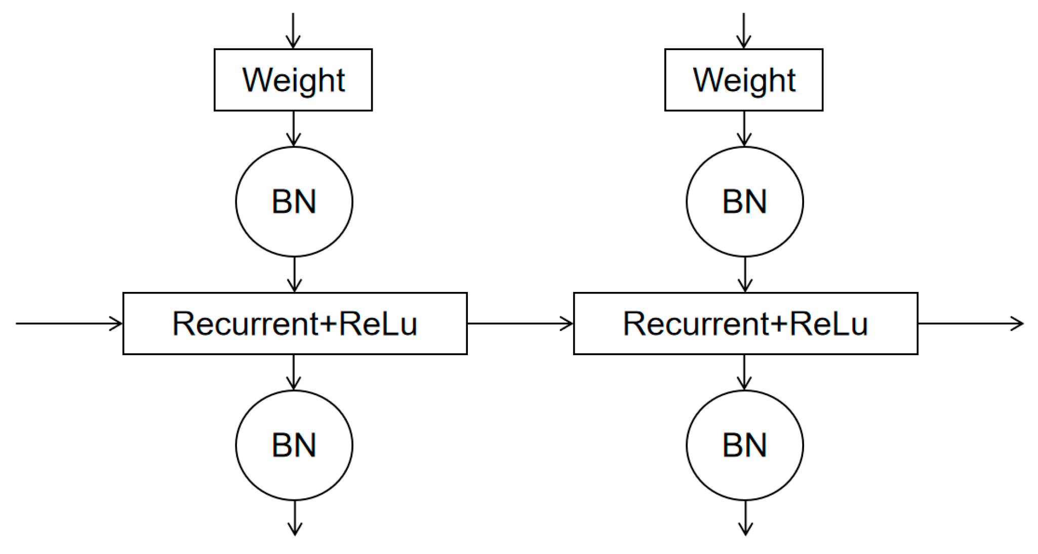
3.2. IndRNN

An independent recurrent neural network is a structure for processing sequential data, which is a variant of a recurrent neural network.

Traditional recurrent neural networks have many problems, such as a vanishing gradient and gradient explosion; neurons within layers are interconnected, making it difficult to provide a reasonable explanation of the neurons’ behavior; LSTM and GRU use Sigmoid and Tanh activation functions, and the gradient decays between the layers, making it difficult to make a multilayer network.

In traditional recurrent neural networks, the update of the hidden state is obtained by weighting the inputs and the hidden state of the previous time step with a weighted activation. The IndRNN, on the other hand, introduces element-by-element updating in this weighting step by performing an element-by-element multiplication operation with the hidden state of the previous time step to adjust the state of the hidden layer. This allows the network to dynamically scale the hidden state changes while processing the sequence data [27,28].

The traditional RNN hidden layer state update formula is:

$$h_t=\sigma (W{x}_t+U{h}_{t-1}+b)$$

(10)

The hidden layer state update formula for the IndRNN is:

$$h_t=\sigma \left(W{x}_t+u\odot h_{t-1}+b\right)$$

(11)

where $h_t$ is the hidden state at time step t, $x_t$ is the input at time step t, W is the input weight matrix, U is the loop weight matrix, u is the loop weight vector, and b is the bias. From Equation (5), it can be seen that in the IndRNN, each neuron at moment t receives only the input of this moment and its own state input at moment t − 1, and each neuron is independent. In contrast, in the RNN, each neuron at moment t has to accept the input of this moment and the state input of all neurons at moment t − 1, and each neuron is not independent. Full connections become passed between individual neurons themselves, as shown schematically in Figure 5.

In order to specifically understand the advantages of the IndRNN, it needs to know the gradient calculation formulas of the traditional RNN and the IndRNN. Firstly, the gradient calculation formula for the RNN is listed, as shown in the Formula (6), and the gradient formula for the IndRNN is then listed, as shown in Formula (7):

$$\frac{\partial J}{\partial h_t}=\frac{\partial J}{\partial h_T}\frac{\partial h_T}{\partial h_t}=\frac{\partial J}{\partial h_T}{\displaystyle \prod _{k=t}^{T-1}diag({\sigma }^{\prime }(h_{k+1}))U^T}$$

(12)

$$\frac{\partial J_n}{\partial h_{n,t}}=\frac{\partial J_n}{\partial h_{n,T}}{\displaystyle \prod _{k=t}^{T-1}\frac{\partial h_{n,k+1}}{\partial h_{n,k}}}=\frac{\partial J_n}{\partial h_{n,T}}{\displaystyle \prod _{k=t}^{T-1}{{\sigma }^{\prime }}_{n,k+1}{u}_n=}\frac{\partial J_n}{\partial h_{n,T}}{u}_n^{T-t}{\displaystyle \prod _{k=t}^{T-1}{{\sigma }^{\prime }}_{n,k+1}}$$

(13)

In the traditional gradient computation formula for RNNs, diag is the Jacobian matrix of the elemental activation functions, and it can be seen that the gradient computation for RNNs relies on the concatenated product of diagonal matrices $diag({\sigma }^{\prime }(h_{k+1}))U^T$. In IndRNNs, the concatenation operation is no longer a matrix operation, the matrix concatenation becomes a power of a number, and the derivatives of the activation function are separated independently from the cyclic weight coefficients. It is only necessary to adjust the exponential term $u_n^{T-t}{\displaystyle \prod _{k=t}^{T-1}{{\sigma }^{\prime }}_{n,k+1}}$ to a suitable range to constrain $u_n$ to avoid the problem of a vanishing gradient or gradient explosion.

The basic architecture of an IndRNN is shown in Figure 6. In this structure, Weight and Recurrent + ReLU are responsible for the processing of input and loop steps, respectively. Both of them use ReLU activation functions and add batch normalization operations before input and output so that they have a more stable distribution. By overlapping this core structure, we can create an IndRNN network with a deep structure.

3.3. Dilated CNN-IndRNN

We combine both a dilated CNN and an IndRNN to construct the dilated CNN-IndRNN combined model, and the specific structure is schematically shown in Figure 7.

The specific parameters of the model network are presented in

Table 1. Network structure setup.

	Layer (Type)	Output Shape	Param
1	Linear_1	[128, 64, 128]	2688
2	LeakyReLU_1	[128, 64, 128]	0
3	Dropout_1	[128, 64, 128]	0
4	IndRNNv2_1	[128, 64, 128]	128
	Conv1d_1_1	[128, 128, 64]	16,512
6	Dropout_2	[128, 64, 128]	0
7	Attention_1	[128, 128]	128
8	Linear_1_1	[128, 64, 128]	16,512
9	BatchNorm1d_1	[128, 128]	256
10	Dropout_3	[128, 64, 128]	0
11	Conv1d_1	[128, 64, 64]	24,640
12	AdaptiveAvgPool1d_1	[128, 64, 1]	0
13	LeakyReLU_2	[128, 64]	0
14	BatchNorm1d_2	[128, 64]	128
15	Linear_2	[128, 128]	24,704
16	Linear_3	[128, 64]	12,352
17	LeakyReLU_3	[128, 192]	0
18	Dropout_3	[128, 192]	0
19	Linear_4	[128, 3]	579

below. The first column is the name of each layer, the second column is the form of output data for each layer, and the third column is the parameter quantity.

4. Results

The parameters need to be set before the model training. The following is the selection of some parameters and the final parameters.

The learning rate is an important hyper-parameter to control the update step of model parameters when training neural networks. The role of the learning rate is mainly reflected in the optimization algorithm, which adjusts the update speed of the model parameters to make the model converge to the optimal solution or local optimal solution faster during the training process. A smaller learning rate will make the parameter update rate smaller, so that the convergence speed of the model is slower, but it helps to avoid skipping the optimal solution. A larger learning rate will make the parameter update larger, which may lead to the instability or even divergence of the optimization process. The following four values of the learning rate 0.1, 0.01, 0.001, 0.0001 are selected for testing. Among them, the learning rate 0.1 cannot converge, so it is not drawn in Figure 8. The model has the best performance when the learning rate is 0.001.

The number of convolutional layers is set to 1, 2, 3, and 4 layers, respectively, and the performance of the model under different numbers of convolutional layers is analyzed. The performance indicators of different convolutional layer models are shown in Figure 9. It can be found that the number of convolutional layers has little effect on the performance of the model. When the number of convolutional layers increases, the performance of the model is slightly improved. When the number of convolution layers is 4, the model has the best performance.

After the hyper-parameter optimization settings, the results of each parameter are shown in

Table 2. Comparison table for different sequence lengths and batch sizes.

Sequence Length	Batch Size	Acc
32	64	91.74
32	128	91.38
32	256	91.16
64	64	92.54
64	128	92.39
64	256	92.32
128	64	93.12
128	128	92.98
128	256	92.43
256	64	93.01
256	128	92.76
256	256	92.68

.

The dilated CNN-IndRNN model was used to set different sequence lengths and batch sizes for comparison. The comparison results are shown in Table 1. When the sequence length is 128 and the batch size is 64, the model has the best running effect, and the accuracy rate reaches 93.12%.

The dilated CNN increases the receptive field of the convolution kernel by introducing a dilation rate without increasing the additional computational cost or the number of parameters. The expansion rate determines the spacing between the points in the convolution kernel. In the dilated convolution, an expansion rate of 1 means the standard convolution operation, and an expansion rate greater than 1 means that there will be holes between the elements of the convolution kernel so that the convolution kernel covers a larger input area. Set the convolution expansion rate to 2, 3, and 4 for comparative experiments, as shown in

Table 3. Comparison of different dilation rates.

Dilation Rate	Acc
2	92.45
3	93.04
4	92.88
5	92.37

. The value of the expansion rate has an effect on the overall performance of the model. When the expansion rate is set to 3, the performance of the model is the best. When the value is greater than 3, the accuracy begins to decline.

After the hyper-parameter optimization settings, the results of each parameter are shown in

Table 4. Parameter setting table.

	Parameters	Numerical Value
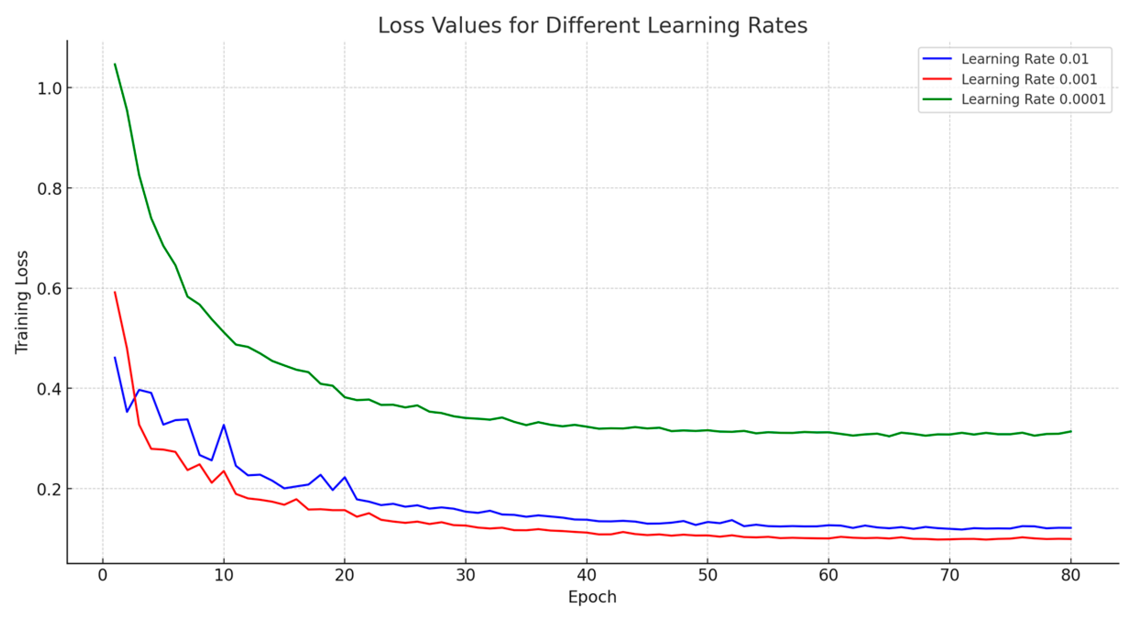
1	Learning Rate	0.001
2	Batch size	64
3	Sequence length	128
4	Epochs	80
5	Optimizer	Adam
6	Dilation rate	3
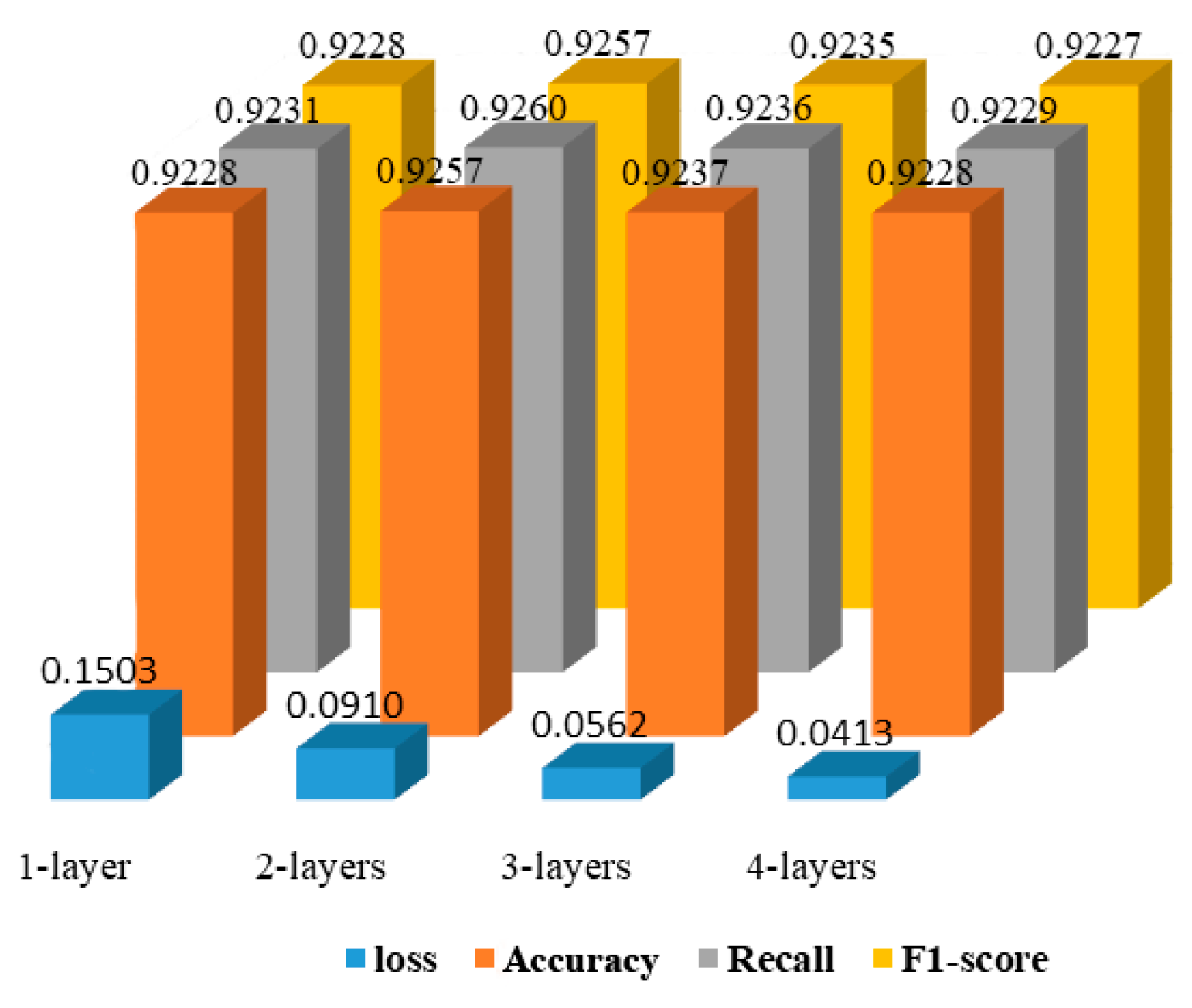
7	Number of convolution layers	4

.

According to the selected parameters brought into the model, the training results accuracy graph and loss graph are obtained, as shown in Figure 10 and Figure 11. The abscissa in the diagram is epoch, and the ordinate is the accuracy and loss value. The accuracy gradually increases with the increase in epoch, and the loss value gradually decreases with the increase in epoch, and finally, tends to converge.

This study selected a separate dilated CNN model, an Ind RNN model, a CNN model, LSTM, and other models for comparative analysis, and also selected some models studied by other scholars. The summary of their respective model evaluation indicators is shown in

Table 5. Comparison table of model results.

Model	Acc	Pre	macro-F1	Recall
Dilated CNN	0.8874	0.8880	0.8869	0.8882
IndRNN	0.9090	0.9099	0.9094	0.9101
CNN-LSTM	0.9156	0.9132	0.9122	0.9124
Dilated CNN-IndRNN	0.9312	0.9310	0.9310	0.9314
CNN	0.8687	0.8692	0.8677	0.8694
LSTM	0.9076	0.9103	0.9068	0.9066
Transformer	0.8956	0.8949	0.8960	0.8950
TCN	0.8645	0.8631	0.8630	0.8645
GRU	0.8663	0.8649	0.8642	0.8657
Bi-LSTM	0.8905	0.8897	0.8898	0.8903
Bi-GRU	0.8725	0.8728	0.8715	0.8713
RNN	0.8587	0.8571	0.8582	0.8569
LightGBM	0.9301	0.9208	0.9168	0.9064
ConvLSTM	0.9105	0.9102	0.9111	0.9106

. Among them, accuracy is the proportion of correctly classified instances out of the total instances. Precision is the proportion of true positive instances among all predicted positive instances. It focuses on the accuracy of positive predictions. Recall is the proportion of true positive instances that were correctly identified by the model. It measures the ability of the model to capture all relevant instances. The F1 score is the harmonic mean of precision and recall. It provides a balance between precision and recall. Compared with other models, we can find that the model proposed in this work is the best working model based on all indicators.

The receiver operating characteristic curve and the area under curve are graphical indicators for evaluating the performance of binary classification models. The ROC curve is a curve with the false positive rate as the abscissa and the true positive rate as the ordinate, which is used to evaluate the performance of the binary classification model under different thresholds. The AUC value is the area under the ROC curve, which is used to measure the ability of the model to sort the samples. The larger the AUC value, the better the model performance. The curves of the dilated CNN-IndRNN model are shown in Figure 12. All three ROC curves of the model are close to the upper left corner, and the area under the ROC curve is close to 1, indicating that the model classifies well and is able to perform the fishing vessel classification task well.

The confusion matrix is a kind of evaluation index of a machine learning model. It is a two-dimensional matrix, in which rows represent real categories, and columns represent predicted categories. The value of each cell represents the number of samples predicted by the model on the test set as a certain category, and the value in the diagonal cell is the correct number of predictions. The confusion matrix heat map visualization can intuitively represent the predicted distribution of the model and use the depth of the color to represent the size of the value. The confusion matrix plot for the dilated CNN-IndRNN model listed below is shown in Figure 13, where it can be seen that the classification of the dilated CNN-IndRNN model is excellent.

5. Discussion

Marine resources are one of the most important resources in China and play an important role in China’s economic development. How to make sustainable use of marine resources is a difficult problem we need to face together. Among them, accurate identification of fishing vessel operation types can combat illegal fishing and help relevant departments in formulating fishery policies, which is the key to protecting marine resources.

In this study, a dilated CNN-IndRNN model combining a dilated convolution (dilated CNN) and an independently recurrent neural network (IndRNN) was built for the first time. The CNN is improved to a dilated CNN, and the dilation rate is added so that it can focus on a wider range of features in long-sequence tasks. The improvement of LSTM to IndRNN changes the connection mode of neurons so that it can avoid gradient disappearance or explosion when capturing long-term dependencies. The experimental results show that the accuracy rate of the improved model is 93.18%, the precision rate is 93.17%, the recall rate is 93.22%, and the F1 score is 93.18%.

According to the experimental results, it can be found that the performance of the model is improved after the CNN is improved to a dilated CNN. This shows that the introduction of the dilation rate and the expansion of the receptive field improve the model’s ability to extract features. After improving LSTM to IndRNN, the performance of the model is greatly improved. This shows that the simple structure of the IndRNN is more suitable for long time series tasks and is important for capturing long-term dependencies. The IndRNN is more important than the dilated CNN for improving the performance of the combined model because the performance of the IndRNN alone is already relatively high. However, the introduction of a dilated CNN can further improve the performance of the model, which shows that in this combination, each part contributes to the performance of the model in a unique way, in which the contribution of the IndRNN is more prominent, but the role of the dilated CNN cannot be ignored, and the two together constitute a powerful combination model.

Although the model has high accuracy in the identification of fishing vessel operation types, there are still some deficiencies. First of all, because the classification of fishing vessels by data sources is limited to three categories, future research can increase the types of fishing vessels. Secondly, future research can increase the data verification of field fishing vessel operation types in multiple regions and increase the persuasiveness of the article.

6. Conclusions

According to the time series characteristics of fishing vessel trajectory data, this paper proposes a method to classify fishing vessel types using the dilated CNN-IndRNN model. This method takes the speed, direction, longitude, and latitude of the fishing vessel trajectory data as input and makes full use of the time series characteristics of the trajectory data. The experimental results show that compared with CNN, LSTM, dilated CNN, IndRNN, and CNN-LSTM, dilated CNN-IndRNN has the highest prediction accuracy and the best performance.

In the future, the model can be applied in the field of combating illegal fishing. At present, different fishing regulations are adopted for different types of fishing vessels in some areas, which limits the area and time of fishing. This model can accurately identify the type of operation of each fishing vessel so as to judge illegal fishing behavior. At the same time, the fishing area can be judged, and the aggregation area of different types of fish can be preliminarily determined according to the aggregation area of different types of fishing boats. Finally, the classification of fishing vessel operation types by this model can provide basic data for other studies and help in carrying out deeper research tasks.

References

- Worm, B.; Hilborn, R.; Baum, J.K.; Branch, T.A.; Collie, J.S.; Costello, C.; Fogarty, M.J.; Fulton, E.A.; Hutchings, J.A.; Jennings, S.; et al. Rebuilding global fisheries. Science 2009, 325, 578–585. [Google Scholar] [CrossRef]
- Duarte, C.M.; Agusti, S.; Barbier, E.; Britten, G.L.; Castilla, J.C.; Gattuso, J.P.; Fulweiler, R.W.; Hughes, T.P.; Knowlton, N.; Lovelock, C.E.; et al. Rebuilding marine life. Nature 2020, 580, 39–51. [Google Scholar] [CrossRef] [PubMed]
- Kasperski, S.; Holland, D.S. Income diversification and risk for fishermen. Proc. Natl. Acad. Sci. USA 2013, 110, 2076–2081. [Google Scholar] [CrossRef] [PubMed]
- Macfadyen, G.; Huntington, T.; Cappell, R. Abandoned, Lost or Otherwise Discarded Fishing Gear; FAO Fisheries and Aquaculture Technical Paper No. 523; FAO: Rome, Italy, 2009. [Google Scholar]
- Sumaila, U.R.; Lam, V.W.; Miller, D.D.; Teh, L.; Watson, R.A.; Zeller, D.; Cheung, W.W.; Côté, I.M.; Rogers, A.D.; Roberts, C.; et al. Winners and losers in a world where the high seas is closed to fishing. Sci. Rep. 2019, 9, 8481. [Google Scholar] [CrossRef] [PubMed]
- Zhang, Y.; Guo, H.; Shi, Q. Anomaly Detection of Fishing Vessels Based on AIS Data. IEEE Access 2020, 8, 131682–131694. [Google Scholar]
- Rashidi, T.H.; Qiu, Z.; Lin, T. Detecting suspicious fishing vessel behaviors from AIS data using deep learning. IEEE Access 2021, 9, 30188–30200. [Google Scholar]
- Sun, L.; Li, C.; Shen, S. Detecting Illegal Fishing Vessels Using Automatic Identification System Data Based on Machine Learning Algorithms. Ocean Eng. 2020, 211, 107580. [Google Scholar]
- O’Neill, F.G.; Handegard, N.O.; Gargan, P.G. Use of a Vessel Monitoring System (VMS) to improve spatial management measures for a data-poor deep-water fishery. ICES J. Mar. Sci. 2019, 76, 1766–1777. [Google Scholar]
- Solomon, J.A.; Cox, S.P.; Carr-Harris, C. Validation of GPS loggers and vessel monitoring systems for use on fishing vessels. Fish. Res. 2020, 230, 105648. [Google Scholar]
- Teixeira, J.B.; Santana, J.A.; Pennino, M.G. A systematic approach to identify fishing areas based on VMS data: Application to the Brazilian pair trawl fishery targeting Argentine hake. Fish. Res. 2019, 215, 1–9. [Google Scholar]
- Ibrahim, H.; Haroun, R.; Moustafa, M. Evaluation of trawling, gillnetting and longlining fishing gear efficiency and sustainability in the Red Sea. Fish. Res. 2019, 209, 30–41. [Google Scholar]
- Campbell, R.A.; Walmsley, S.F.; Robinson, G. Fishing gear classification based on fish behaviour to assist fisheries management. Fish. Res. 2013, 147, 428–441. [Google Scholar]
- Ulman, A.; Bekişoğlu, Ş.; Moutopoulos, D.K. The impact of trawl fishery on the ecosystem in the south-eastern Black Sea. J. Mar. Biol. Assoc. UK 2015, 95, 1051–1061. [Google Scholar]
- Kroodsma, D.A.; Mayorga, J.; Hochberg, T.; Miller, N.A.; Boerder, K.; Ferretti, F.; Wilson, A.; Bergman, B.; White, T.D.; Block, B.A. Tracking the global footprint of fisheries. Science 2018, 359, 904–908. [Google Scholar] [CrossRef] [PubMed]
- Kim, K.L.; Lee, K.M. Convolutional neural network based geartype ide-ntification from automatic identification system trajectory data. Appl. Sci. 2020, 10, 4010. [Google Scholar] [CrossRef]
- Storm-Furru, S.; Bruckner, S. VA-TRAC: Geospatial Trajectory Analysis for Monitoring, Identification, and Verification in Fishing Vessel Operations. Comput. Graph. Forum 2020, 39, 101–114. [Google Scholar] [CrossRef]
- Park, J.W.; Lee, K.M.; Kim, K.I. Automatic identifica-tion system based fishing trajectory data preprocessing method using map reduce. Int. J. Recent Technol. Eng. 2019, 8, 352–356. [Google Scholar]
- De Souza, E.N.; Boerder, K.; Matwin, S.; Worm, B. Improving Fishing Pattern Detection from Satellite AIS Using Data Mining and Machine Learning. PLoS ONE 2017, 11, e0158248. [Google Scholar]
- Candela, L.; Arvanitidis, C. Challenges and opportunities in using vessel monitoring systems and automatic identification systems (VMS/AIS) to support the ecosystem approach to fisheries. Aquat. Conserv. Mar. Freshw. Ecosyst. 2017, 27, 156–167. [Google Scholar]
- Powell, M.J.D. A hybrid method for nonlinear equations. Numer. Methods Nonlinear Algebr. Equ. 1981, 12, 663–683. [Google Scholar]
- Yao, Y.; Jiang, Z.; Zhang, H. Ship detection in optical remote sensing images based on deep convolutional neural networks. J. Appl. Remote Sens. 2017, 11, 042611. [Google Scholar] [CrossRef]
- Bono, F.M.; Cinquemani, S.; Chatterton, S.; Pennacchi, P. A deep learning approach for fault detection and RUL estimation in bearings. In NDE 4.0, Predictive Maintenance, and Communication and Energy Systems in a Globally Networked World, Proceedings of the SPIE Smart Structures + Nondestructive Evaluation, Long Beach, CA, USA, 18 April 2022; SPIE: Bellingham, WA, USA, 2022; Volume 12049, pp. 71–83. [Google Scholar]
- LeCun, Y.; Bengio, Y.; Hinton, G. Deep learning. Nature 2015, 521, 436–444. [Google Scholar] [CrossRef]
- Goodfellow, I.; Bengio, Y.; Courville, A. Deep Learning; MIT Press: Cambridge, MA, USA, 2016; Volume 1. [Google Scholar]
- Arai, T.; Watanabe, S.; Hotta, K. Convolutional neural networks for super-resolution of raw time-of-flight depth images. IEEE Trans. Image Process. 2017, 26, 4226–4237. [Google Scholar]
- Li, S.; Li, W.; Cook, C. Independently Recurrent Neural Network (IndRNN): Building A Longer and Deeper RNN. In Proceedings of the IEEE Conference on Computer Vision and Pattern Recognition, Salt Lake City, UT, USA, 18–22 June 2018; pp. 5457–5466. [Google Scholar]
- Li, Y.; Hu, S.; Zhang, J. IndRNN for Time Series Forecasting: A Case Study of Debris Flow Forecasting. Remote Sens. 2020, 12, 2882. [Google Scholar]