
Identification of Milling Cutter Wear State under Variable Working Conditions Based on Optimized SDP

Abstract
1. Introduction
2. The Analysis of SDP’s Characteristics
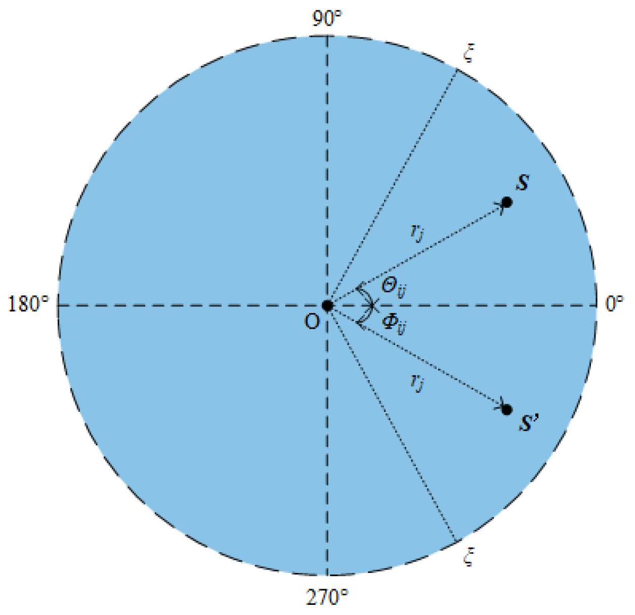
2.1. The Basic Principle of SDP
2.2. The Impact of Different Parameters on the Effect of the SDP Transformation
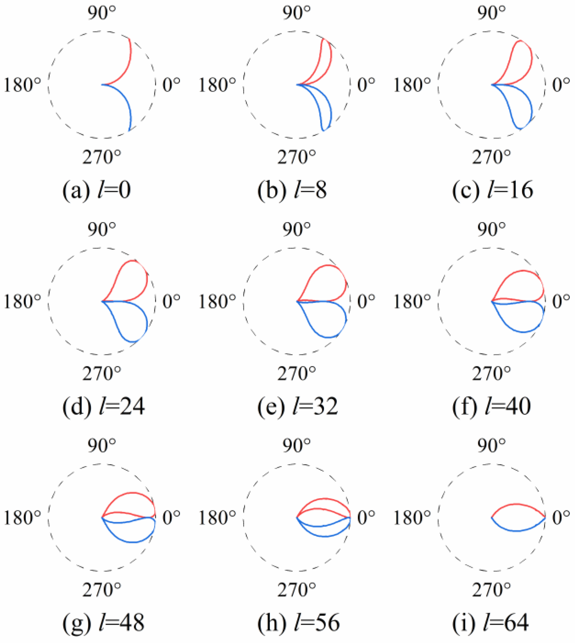
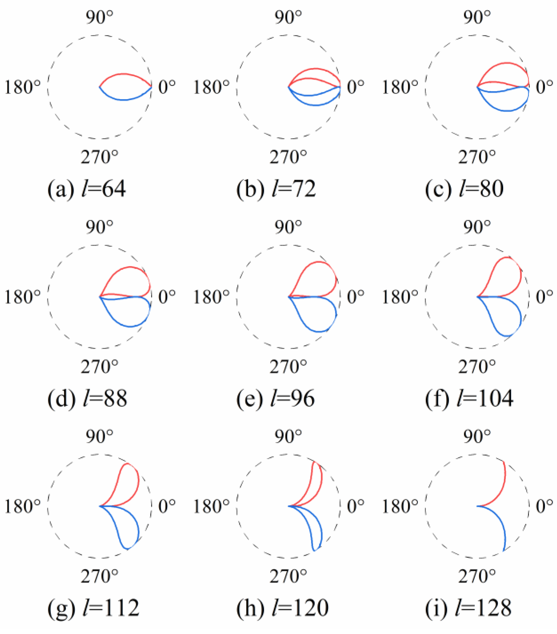
- The impact of the lag coefficient l on the SDP transformation effect.
- 2.
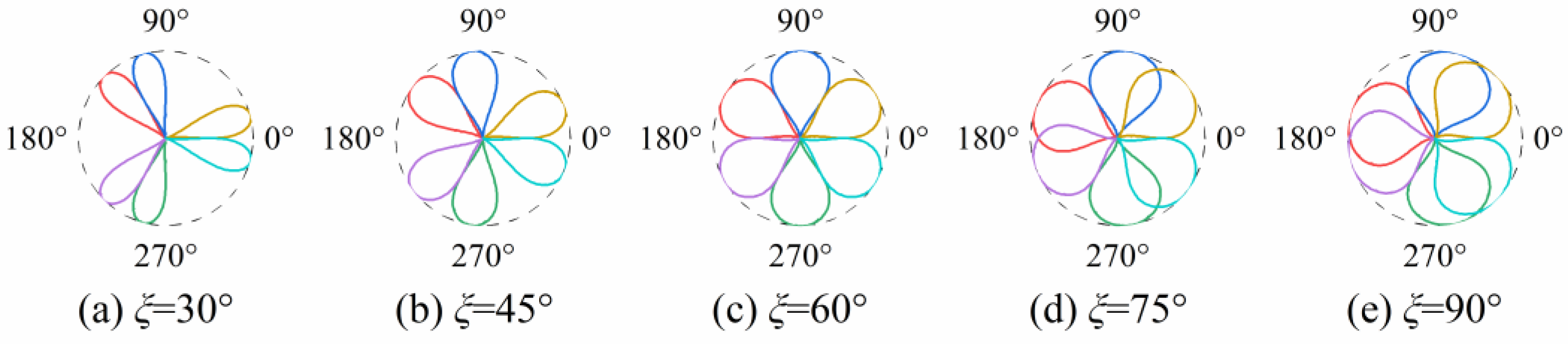
- The impact of the aperture gain ξ on the SDP transformation effect.
3. Recognizing the Wear State of Milling Cutters under Variable Conditions Based on Optimized SDP
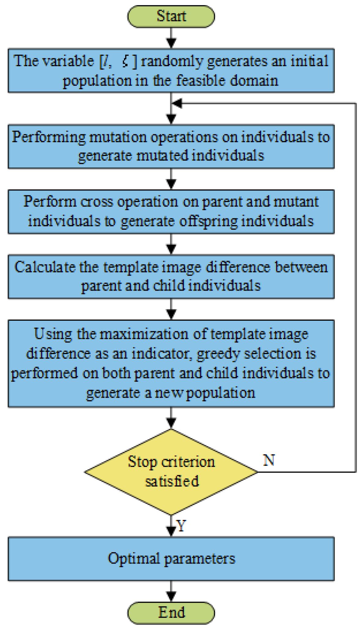
3.1. Optimization of SDP Parameters Based on the Differential Evolution Algorithm
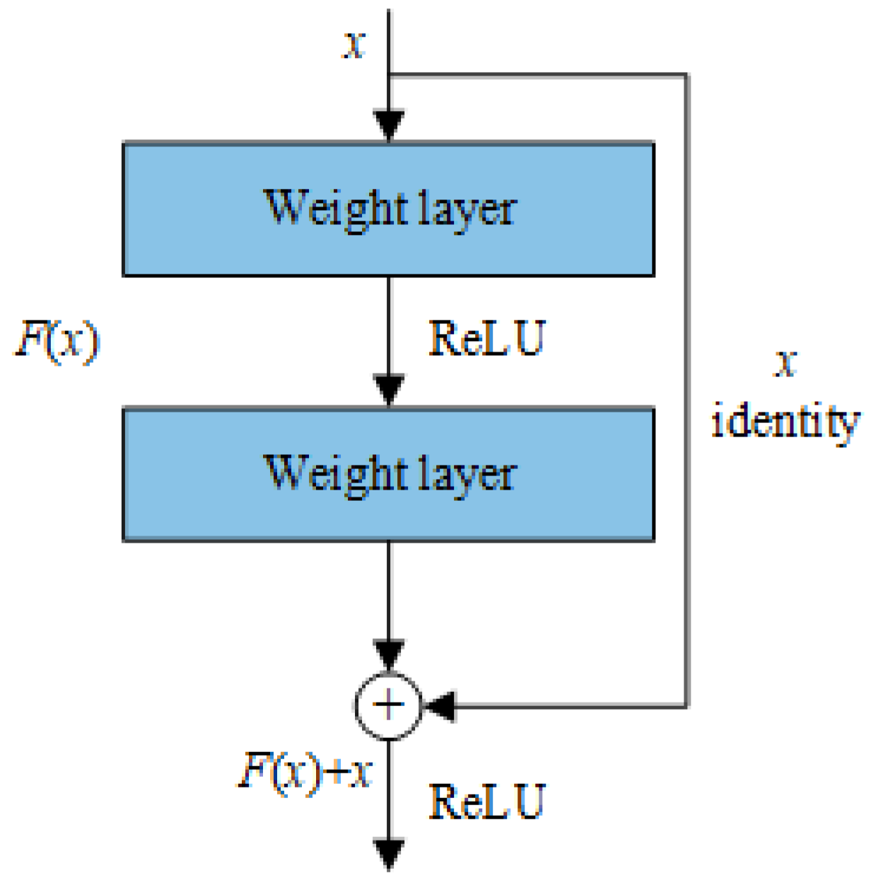
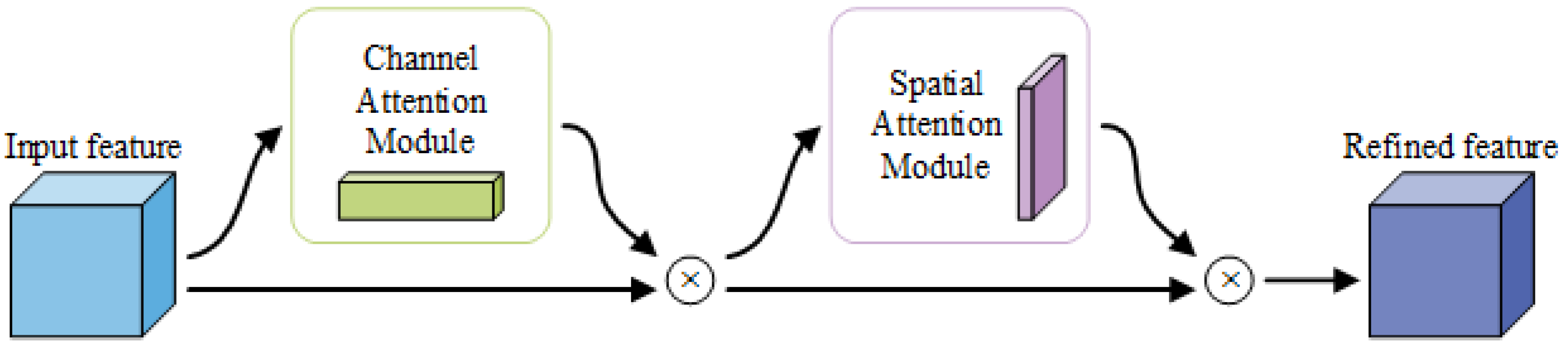
3.2. A Residual Network with an Integrated Attention Mechanism
3.3. The Process of Recognizing the Wear State of Milling Cutters under Variable Conditions Based on Optimized SDP
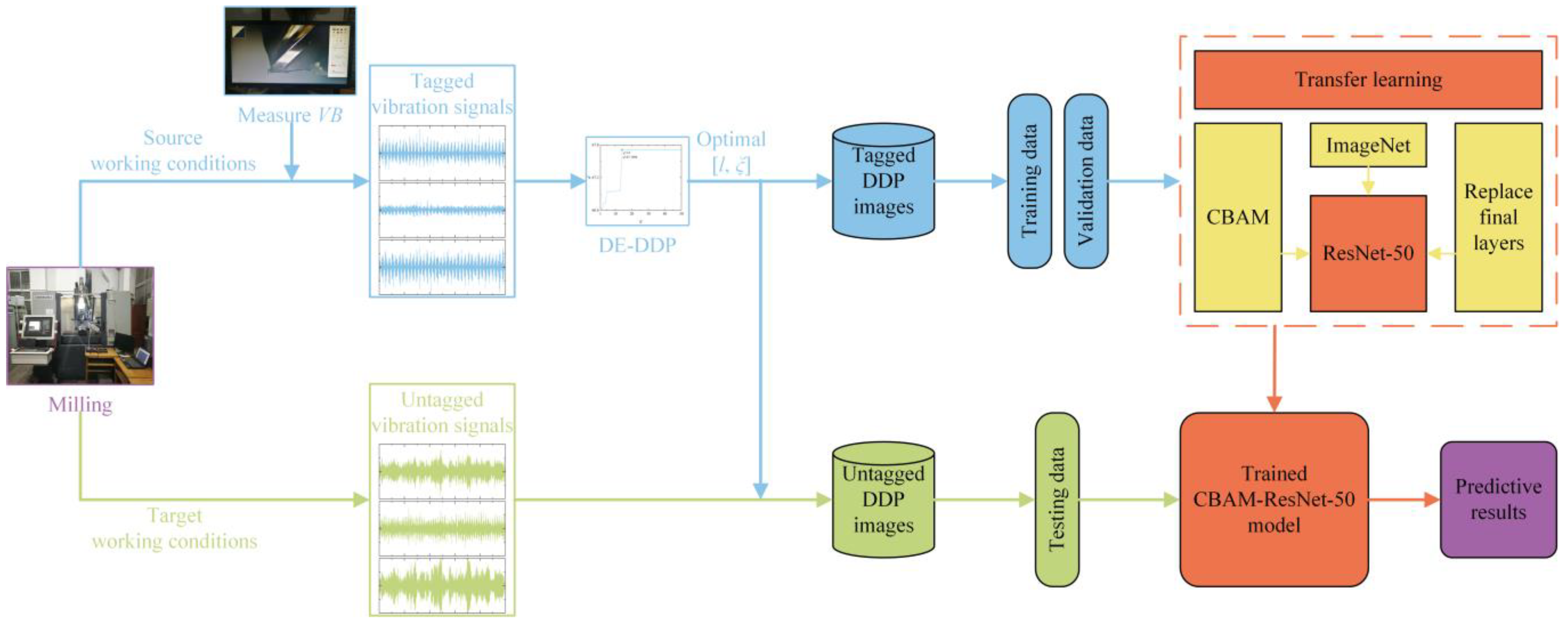
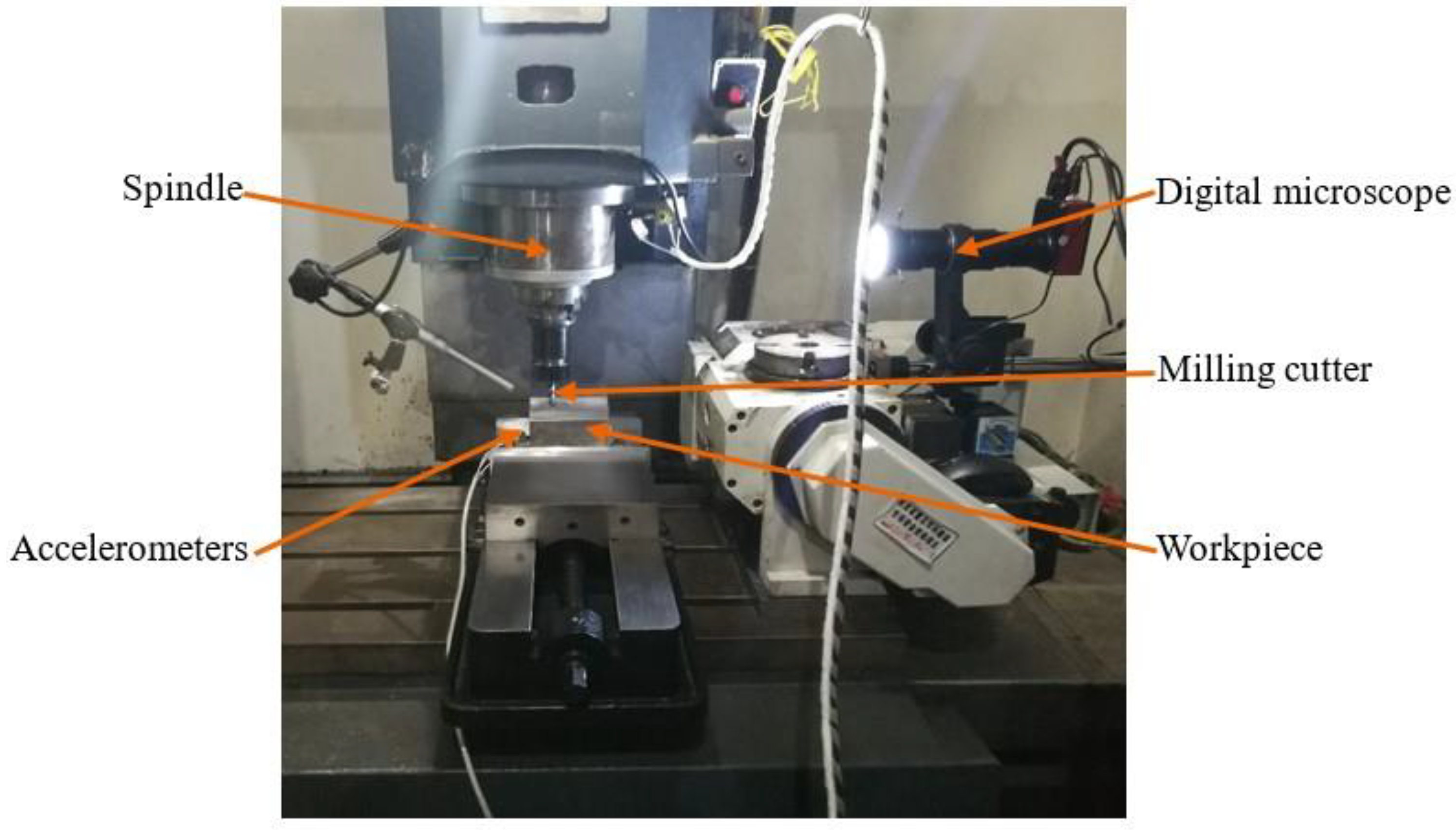
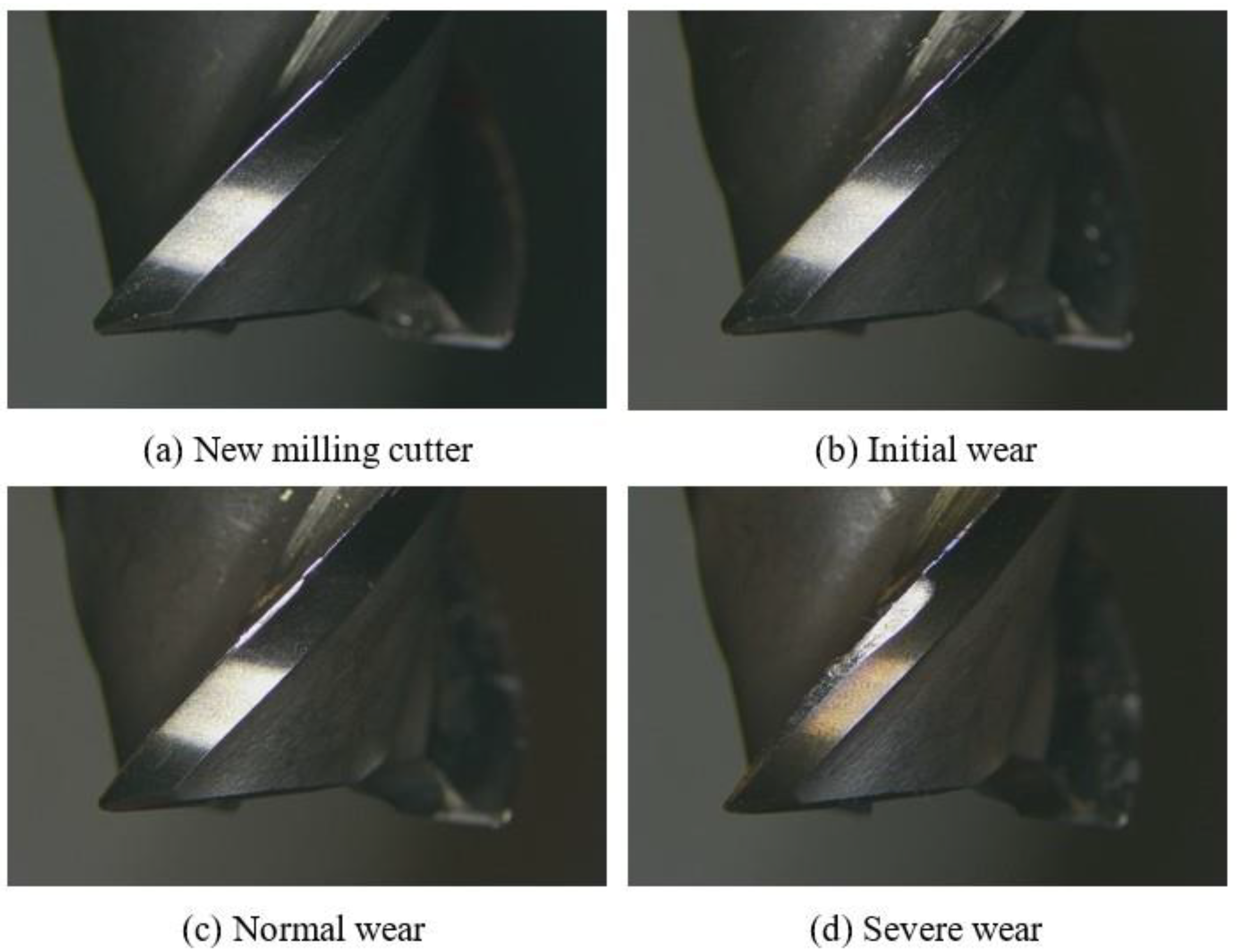
- Collect vibration signals of milling cutters in the initial wear, normal wear, and severe wear stages under different working conditions, and measure the corresponding milling cutter wear amount;
- Use cluster analysis to extract template images for each wear state, with the maximization of differences between template images of each wear state as an indicator, and employ DE to search for the optimal parameter combination [l, ξ] for DDP transformation of milling vibration signals;
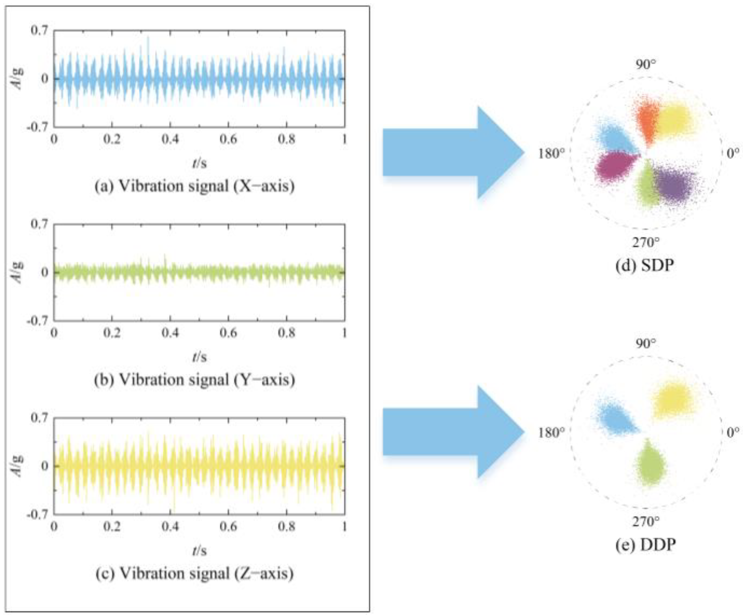
- Use the optimal parameter combination [l, ξ] to perform DDP transformation of milling vibration signals, merging vibration signals from three-axis directions into visualized DDP images;
- Utilize the ResNet-50 model pre-trained on the ImageNet dataset, introduce CBAM, and construct the CBAM-ResNet-50 model;
- Replace the final layer in the CBAM-ResNet-50 model, perform representational learning on DDP images of complete data under source conditions, and fine-tune to form a generalized milling cutter wear state recognition model;
- Classify DDP images of vibration signals under target conditions to identify the wear state of milling cutters in variable condition scenarios.
4. Milling Cutter Wear Experiment and Analysis of Recognition Results
5. Conclusions
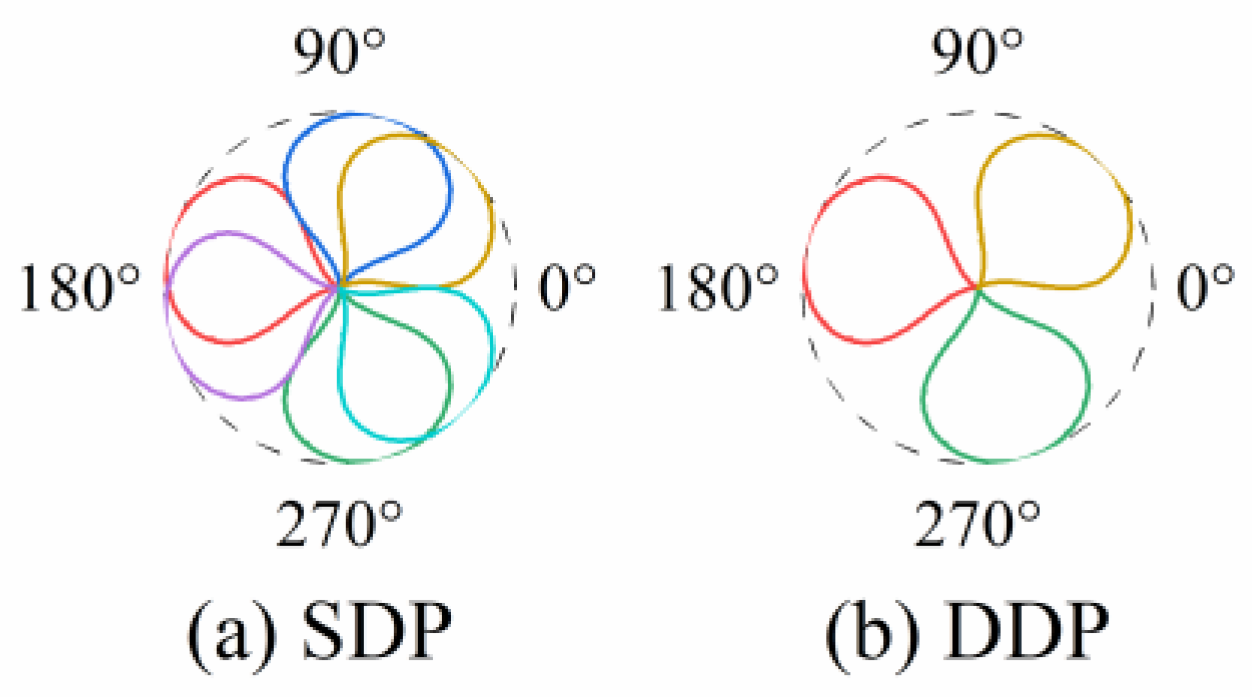
- The vibration signals in milling operations can be transformed from one-dimensional time series to two-dimensional images using SDP transformation, merging vibration signals from the X, Y, and Z axes based on their time series in a designated area to form a unified feature representation. Using a desymmetrization dot pattern effectively avoids overlapping adjacent spiral arms from different mirrors due to parameter selection, aiding in finding optimal parameters.
- Using cluster analysis to extract template images for each wear state, with Euclidean distance maximization as an indicator, adaptively optimizes the selection of SDP parameters l and ξ using the differential evolution algorithm. This effectively solves the problem of SDP transformation effects being limited by preset parameter selection, narrows the intra-class distance, and expands the inter-class difference, thus facilitating the construction of a generalized decision boundary and reducing the impact of working condition changes on the milling cutter wear state mapping relationship.
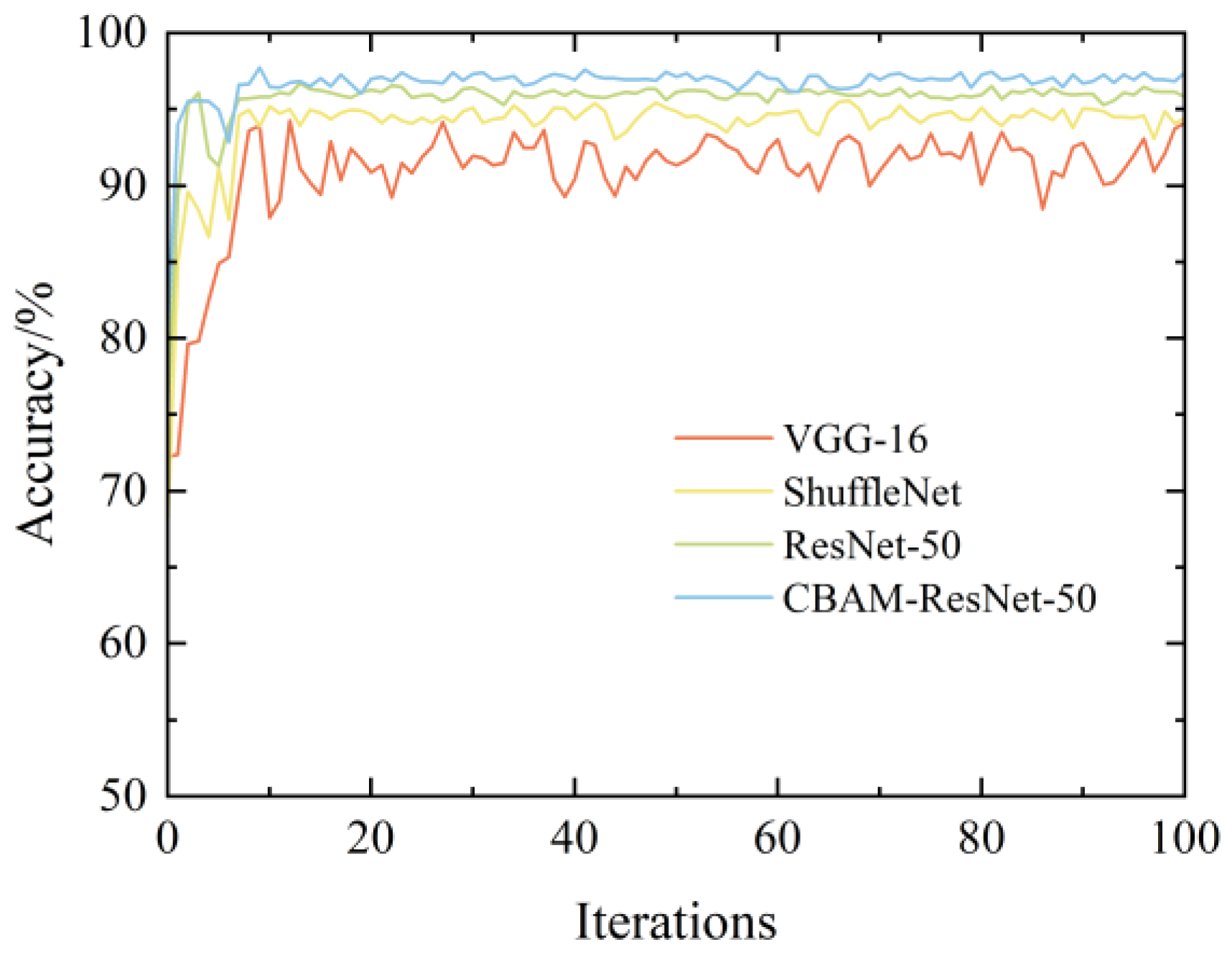
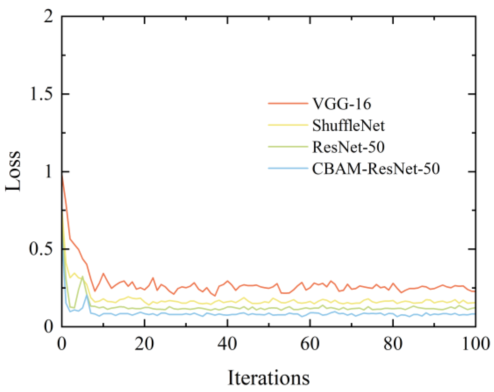
- The use of the CBAM-ResNet-50 network for feature learning of images under source conditions constructs a generalized milling cutter wear state recognition model. The results show that the recognition accuracy for test samples under variable conditions can reach over 95%. This method can effectively use labeled data from source conditions to classify unlabeled data from target conditions, achieving the recognition of milling cutter wear states in variable condition scenarios with good recognition accuracy and generalization ability.
Author Contributions
Funding
Institutional Review Board Statement
Informed Consent Statement
Data Availability Statement
Conflicts of Interest
References
- Sarıkaya, M.; Gupta, M.K.; Tomaz, I.; Pimenov, D.Y.; Kuntoglu, M.; Khanna, N.; Yıldırım, Ç.V.; Krolczyk, G.M. A state-of-the-art review on tool wear and surface integrity characteristics in machining of superalloys. CIRP J. Manuf. Sci. Technol. 2021, 35, 624–658. [Google Scholar] [CrossRef]
- Yu, W.N.; Mechefske, C.; Kim, I.Y. Identifying optimal features for cutting tool condition monitoring using recurrent neural networks. Adv. Mech. Eng. 2020, 12, 1687814020984388. [Google Scholar] [CrossRef]
- Pálmai, Z. Proposal for a new theoretical model of the cutting tool’s flank wear. Wear 2013, 303, 437–445. [Google Scholar] [CrossRef]
- Cheng, Y.N.; Guan, R.; Lu, Z.Z.; Xu, M.; Liu, Y.Z. A study on the milling temperature and tool wear of difficult-to-machine 508III steel. Proc. Inst. Mech. Eng. Part B-J. Eng. Manuf. 2017, 232, 2478–2487. [Google Scholar] [CrossRef]
- Yuan, J.; Liu, L.B.; Yang, Z.Q.; Bo, J.D.; Zhang, Y.R. Tool wear condition monitoring by combining spindle motor current signal analysis and machined surface image processing. Int. J. Adv. Manuf. Technol. 2021, 116, 2697–2709. [Google Scholar] [CrossRef]
- Kong, D.D.; Chen, Y.J.; Li, N.; Duan, C.Q.; Lu, L.X.; Chen, D.X. Relevance vector machine for tool wear prediction. Mech. Syst. Signal Proc. 2019, 127, 573–594. [Google Scholar] [CrossRef]
- Wang, J.J.; Li, Y.L.; Zhao, R.; Gao, R.X. Physics guided neural network for machining tool wear prediction. J. Manuf. Syst. 2020, 57, 298–310. [Google Scholar] [CrossRef]
- Zhou, Y.Q.; Sun, B.T.; Sun, W.F.; Lei, Z. Tool wear condition monitoring based on a two-layer angle kernel extreme learning machine using sound sensor for milling process. J. Intell. Manuf. 2022, 33, 247–258. [Google Scholar] [CrossRef]
- Hesser, D.F.; Markert, B. Tool wear monitoring of a retrofitted CNC milling machine using artificial neural networks. Manuf. Lett. 2019, 19, 1–4. [Google Scholar] [CrossRef]
- Cheng, M.H.; Jiao, L.; Yan, P.; Jiang, H.S.; Wang, R.B.; Qiu, T.Y.; Wang, X.B. Intelligent tool wear monitoring and multi-step prediction based on deep learning model. J. Manuf. Syst. 2022, 62, 286–300. [Google Scholar] [CrossRef]
- Liang, Y.; Hu, S.S.; Guo, W.S.; Tang, H.Q. Abrasive tool wear prediction based on an improved hybrid difference grey wolf algorithm for optimizing SVM. Measurement 2022, 187, 110247. [Google Scholar] [CrossRef]
- He, Z.P.; Shi, T.L.; Xuan, J.P. Milling tool wear prediction using multi-sensor feature fusion based on stacked sparse autoencoders. Measurement 2022, 190, 110719. [Google Scholar] [CrossRef]
- Li, X.B.; Liu, X.L.; Yue, C.X.; Liu, S.Y.; Zhang, B.W.; Li, R.Y.; Liang, S.Y.; Wang, L.H. A data-driven approach for tool wear recognition and quantitative prediction based on radar map feature fusion. Measurement 2021, 185, 110072. [Google Scholar] [CrossRef]
- Huang, Z.W.; Zhu, J.M.; Lei, J.T.; Li, X.R.; Tian, F.Q. Tool wear predicting based on multisensory raw signals fusion by reshaped time series convolutional neural network in manufacturing. IEEE Access 2019, 7, 178640–178651. [Google Scholar] [CrossRef]
- Zhu, G.Q.; Hu, S.S.; Tang, H.Q. Prediction of tool wear in CFRP drilling based on neural network with multicharacteristics and multisignal sources. Compos. Adv. Mater. 2021, 30, 2633366X20987234. [Google Scholar] [CrossRef]
- Qin, Y.R.; Li, J.F.; Zhang, C.X.; Zhao, Q.P.; Ma, X.F. A dual-stage attention model for tool wear prediction in dry milling operation. Entropy 2022, 24, 1733. [Google Scholar] [CrossRef] [PubMed]
- Li, X.B.; Liu, X.L.; Yue, C.X.; Liang, S.Y.; Wang, L.H. Systematic review on tool breakage monitoring techniques in machining operations. Int. J. Mach. Tools Manuf. 2022, 176, 103882. [Google Scholar] [CrossRef]
- Pan, S.J.; Yang, Q. A survey on transfer learning. IEEE Trans. Knowl. Data Eng. 2010, 22, 1345–1359. [Google Scholar] [CrossRef]
- Baskar, C.; Govindasamy, G.P.; Anbalagan, S.; Roomi, S.M.M. Computer graphic and photographic image classification using transfer learning approach. Trait. Signal 2022, 39, 1267–1273. [Google Scholar] [CrossRef]
- Sakallı, G.; Koyuncu, H. Identification of asynchronous motor and transformer situations in thermal images by utilizing transfer learning-based deep learning architectures. Measurement 2023, 207, 112380. [Google Scholar] [CrossRef]
- Tammina, S. Transfer learning using VGG-16 with deep convolutional neural network for classifying images. Int. J. Sci. Res. Publ. 2019, 9, 143–150. [Google Scholar] [CrossRef]
- Zhuang, F.Z.; Qi, Z.Y.; Duan, K.Y.; Xi, D.B.; Zhu, Y.C.; Zhu, H.S.; Xiong, H.; He, Q. A comprehensive survey on transfer learning. Proc. IEEE 2021, 109, 43–76. [Google Scholar] [CrossRef]
- Yuan, W.H.; Lu, X.Y.; Zhang, R.F.; Liu, Y.H. FCKDNet: A feature condensation knowledge distillation network for semantic segmentation. Entropy 2023, 25, 125. [Google Scholar] [CrossRef] [PubMed]
- Mohanraj, T.; Shankar, S.; Rajasekar, R.; Sakthivel, N.R.; Pramanik, A. Tool condition monitoring techniques in milling process—A review. J. Mater. Res. Technol.-JMRT 2020, 9, 1032–1042. [Google Scholar] [CrossRef]
- Mao, G.; Zhang, Z.Z.; Qiao, B.; Li, Y.B. Fusion domain-adaptation CNN driven by images and vibration signals for fault diagnosis of gearbox cross-working conditions. Entropy 2022, 24, 119. [Google Scholar] [CrossRef] [PubMed]
- Wang, M.; Deng, W.H. Deep visual domain adaptation: A survey. Neurocomputing 2018, 312, 135–153. [Google Scholar] [CrossRef]
- Pickover, C.A. On the use of symmetrized dot patterns for the visual characterization of speech waveforms and other sampled data. J. Acoust. Soc. Am. 1986, 80, 955–960. [Google Scholar] [CrossRef] [PubMed]
- Zhang, C.D.; Wang, W.; Li, H. Tool wear prediction method based on symmetrized dot pattern and multi-covariance Gaussian process regression. Measurement 2022, 189, 110466. [Google Scholar] [CrossRef]
- Sun, Y.J.; Li, S.H.; Wang, Y.L.; Wang, X.H. Fault diagnosis of rolling bearing based on empirical mode decomposition and improved manhattan distance in symmetrized dot pattern image. Mech. Syst. Signal Proc. 2021, 159, 107817. [Google Scholar] [CrossRef]
- Xu, X.G.; Liu, H.X.; Zhu, H.; Wang, S.L. Fan fault diagnosis based on symmetrized dot pattern analysis and image matching. J. Sound Vibr. 2016, 374, 297–311. [Google Scholar] [CrossRef]
- Diwakar, A.D.; Manivannan, P.V. Symmetrised dot pattern technique for fault diagnosis in a spur gear assembly using vibration signals. IOP Conf. Ser. Mater. Sci. Eng. 2019, 561, 012079. [Google Scholar] [CrossRef]
- Pang, B.; Liang, J.X.; Liu, H.; Dong, J.H.; Xu, Z.L.; Zhao, X. Intelligent bearing fault diagnosis based on multivariate symmetrized dot pattern and LEG transformer. Machines 2022, 10, 550. [Google Scholar] [CrossRef]


| Diameter of the Cutter | Shank Diameter | Cutting Length | Overall Length | Number of Teeth | Helix Angle |
|---|---|---|---|---|---|
| 10 mm | 10 mm | 22 mm | 72 mm | 3 | 42° |
| Case | ap (mm) | ae (mm) | fz (mm/z) | vc (m/min) |
|---|---|---|---|---|
| 1 | 5 | 0.3 | 0.15 | 23 |
| 2 | 4 | 0.3 | 0.07 | 17 |
| 3 | 3 | 0.5 | 0.07 | 23 |
| 4 | 5 | 0.5 | 0.03 | 29 |
| 5 | 4 | 0.4 | 0.03 | 23 |
| 6 | 3 | 0.2 | 0.03 | 17 |
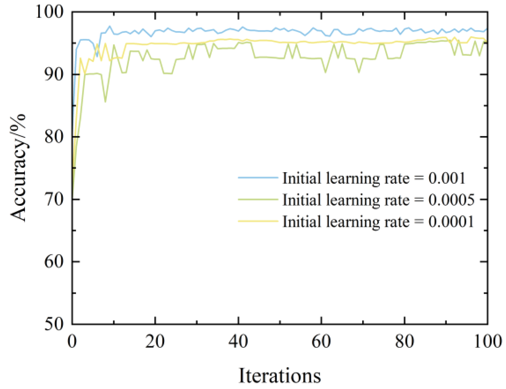
| Initial Learning Rate | Learning Rate Type | Accuracy/% |
|---|---|---|
| 0.001 | fixed learning rate | 94.51 |
| decaying learning rate | 97.39 | |
| 0.0005 | fixed learning rate | 94.1 |
| decaying learning rate | 95.25 | |
| 0.0001 | fixed learning rate | 94.81 |
| decaying learning rate | 95.07 |
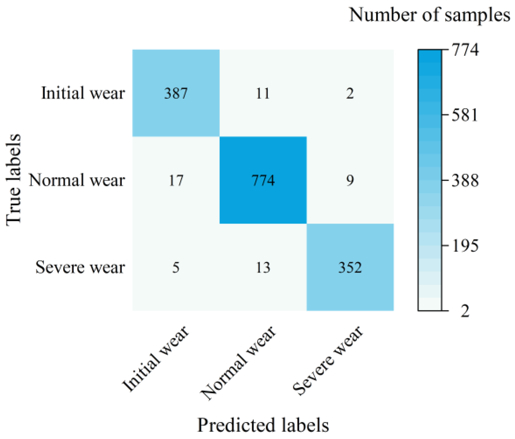
| Milling Cutter Wear States | Precision/% | Recall/% | F1 Score |
|---|---|---|---|
| initial wear | 94.62 | 96.75 | 0.9567 |
| normal wear | 96.99 | 96.75 | 0.9687 |
| severe wear | 96.97 | 95.14 | 0.9605 |
Disclaimer/Publisher’s Note: The statements, opinions and data contained in all publications are solely those of the individual author(s) and contributor(s) and not of MDPI and/or the editor(s). MDPI and/or the editor(s) disclaim responsibility for any injury to people or property resulting from any ideas, methods, instructions or products referred to in the content. |
© 2024 by the authors. Licensee MDPI, Basel, Switzerland. This article is an open access article distributed under the terms and conditions of the Creative Commons Attribution (CC BY) license (https://creativecommons.org/licenses/by/4.0/).
Share and Cite
Chang, H.; Gao, F.; Li, Y.; Chang, L. Identification of Milling Cutter Wear State under Variable Working Conditions Based on Optimized SDP. Appl. Sci. 2024, 14, 4314. https://doi.org/10.3390/app14104314
Chang H, Gao F, Li Y, Chang L. Identification of Milling Cutter Wear State under Variable Working Conditions Based on Optimized SDP. Applied Sciences. 2024; 14(10):4314. https://doi.org/10.3390/app14104314
Chicago/Turabian StyleChang, Hao, Feng Gao, Yan Li, and Lihong Chang. 2024. "Identification of Milling Cutter Wear State under Variable Working Conditions Based on Optimized SDP" Applied Sciences 14, no. 10: 4314. https://doi.org/10.3390/app14104314
APA StyleChang, H., Gao, F., Li, Y., & Chang, L. (2024). Identification of Milling Cutter Wear State under Variable Working Conditions Based on Optimized SDP. Applied Sciences, 14(10), 4314. https://doi.org/10.3390/app14104314