1. Introduction
Situational Awareness (SA) is critical for First Responders (FRs) during rescue operations. FRs must have a clear understanding of the location of individuals in need, any potential risks, and any other essential factors crucial to properly and safely perform their duties. The use of Artificial Intelligence (AI) and advances in object detection technology can greatly enhance FRs’ SA by identifying and highlighting key elements, reducing their cognitive burden, and improving their perception. However, these improvements are effective only in well-lit environments, while, in real-world scenarios, FRs often face challenging conditions, such as smoke, dust, or limited visibility, which can impair both human and AI perception. To overcome these challenges, it is necessary to utilise technology and equip FRs with tools and resources capable to improve their SA in all situations and conditions.
One critical aspect of enhancing FRs’ perceptual ability is to improve their visibility under adverse conditions, such as overexposed and underexposed scenarios. Traditional approaches to image restoration and exposure correction rely on image histogram adjustments. Histogram-based methods operate on the statistical distribution of pixel intensities in an image. These methods modify the histogram to make the image visually appealing and better expose the features in the scene [
1,
2,
3,
4]. Other techniques, related to Retinex theory [
5], have also found wide application, both within and outside of learning-based methodologies [
6,
7,
8,
9,
10,
11]. According to Retinex theory, the perceived colour of an object depends on both the spectral reflectance of the object and the spectral distribution of the incident light. Retinex-based exposure correction algorithms recover the original reflectance of the scene by removing the effects of the illumination. Further research has shown the effectiveness of High Dynamic Range (HDR) based techniques for exposure correction. The most common technique for creating HDR images is to exploit the information of a stack of bracketed exposure Low Dynamic Range (LDR) images [
12,
13,
14,
15]. Other techniques reconstruct an HDR image from a single LDR image [
16,
17,
18,
19,
20].
Despite significant advances in exposure correction techniques, it is essential to note that existing methods are not optimised for rescue scenarios and may not meet the specific needs of FRs. To address this gap, we present a novel pipeline that integrates Deep Learning (DL) and Image-Processing (IP) techniques specifically tailored to improve the operational abilities of rescuers. Our method is designed to meet three main requirements: detailed feature recovery, enhanced object detection, and efficiency. Detailed feature recovery refers to the model’s ability to enhance a scene by revealing hidden features, whereas improved object detection capabilities refer to the model’s capacity to enhance other DL techniques by acting as an intelligence amplification (IA) layer. Furthermore, the pipeline has been designed to handle the high-stress, fast-paced nature of rescue situations, where accurate and quick information is crucial.
As a proof of concept, the pipeline has been tested on a data set created in the framework of the Horizon 2020 project, “first RESponder-Centered support toolkit for operating in adverse and infrastrUcture-less EnviRonments” (RESCUER), during the Earthquake Pilot performed in Weeze, and organised by I.S.A.R Germany (International Search and Rescue organisation).
The paper is structured as follows. In
Section 2, we describe the technical details of the pipeline, including exposure correction, segmentation, and fusion techniques, indicating the DL and IP features involved in the process. We also introduce the data set used, and how we collected the training data. In
Section 3, we present different metrics of model performance validation over the data set constructed in the Weeze Earthquake Pilot. In
Section 4, we discuss the results obtained in
Section 3, highlighting the strengths and potential applications of the proposed approach. Finally, in
Section 5, we summarise the key findings of our study and their implications, as well as highlight limitations and potential areas for future research.
2. Materials and Methods
In rescue operations, the safety of both rescuers and victims relies on having accurate and up-to-date information about the environment. The unpredictable and rapidly changing conditions of a disaster scene make it essential for rescuers to understand the physical and geographical features of the area, as well as any human-made structures or infrastructures present. However, lighting deficiencies and scene degradation can present significant challenges for rescuers in identifying key features, such as pathways, buildings, and other landmarks. To address these challenges, we propose a pipeline that integrates both DL and IP techniques specifically designed to handle extreme lighting conditions. In the following section, the pipeline graphics are depicted using the TM-DIED: The Most Difficult Image Enhancement Dataset [
21], which showcases images in various lighting scenarios featuring diverse intensity shifts between regions that are underexposed, overexposed, and correctly exposed.
2.1. Pipeline Design
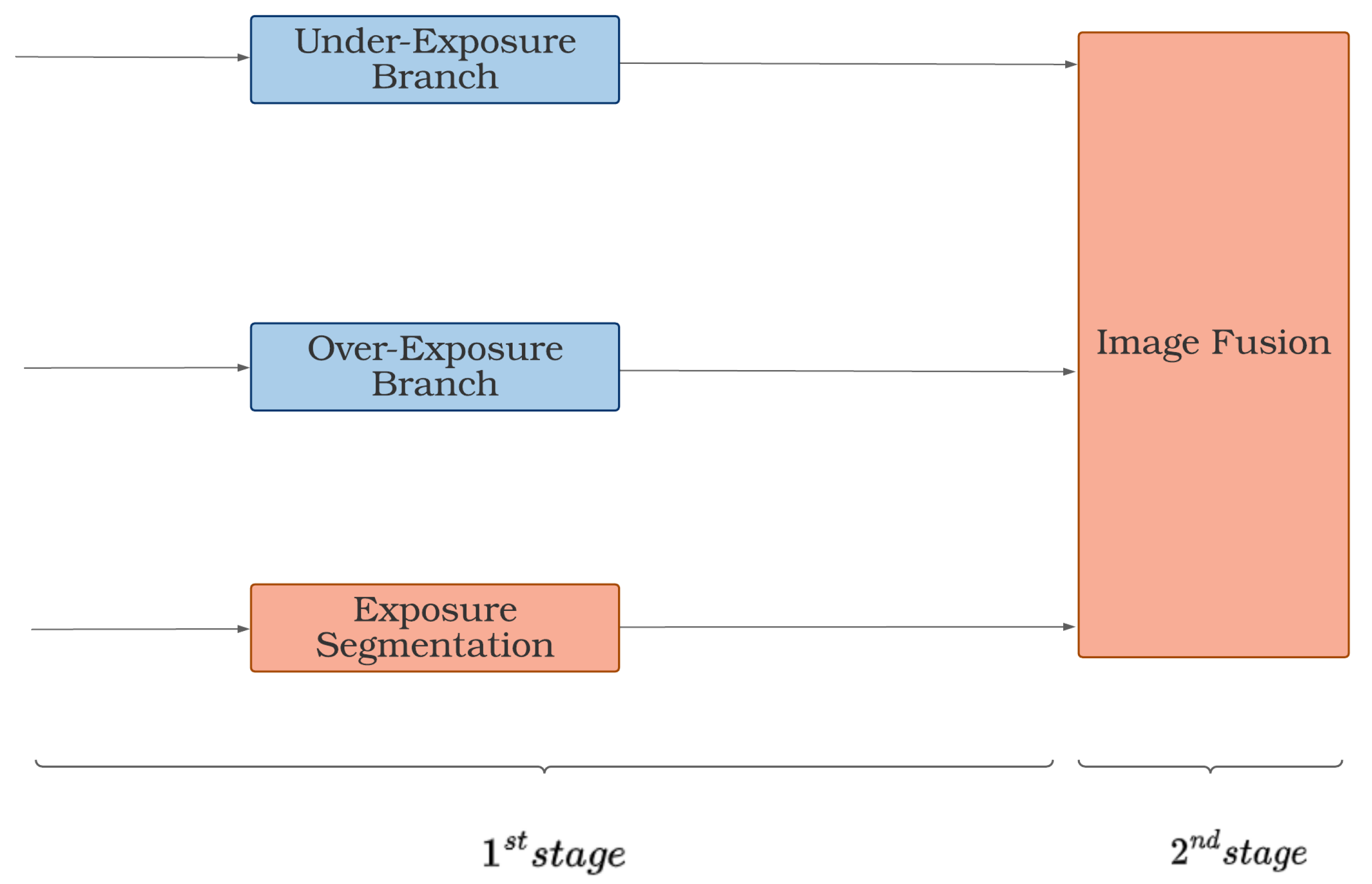
The pipeline, as it is represented in
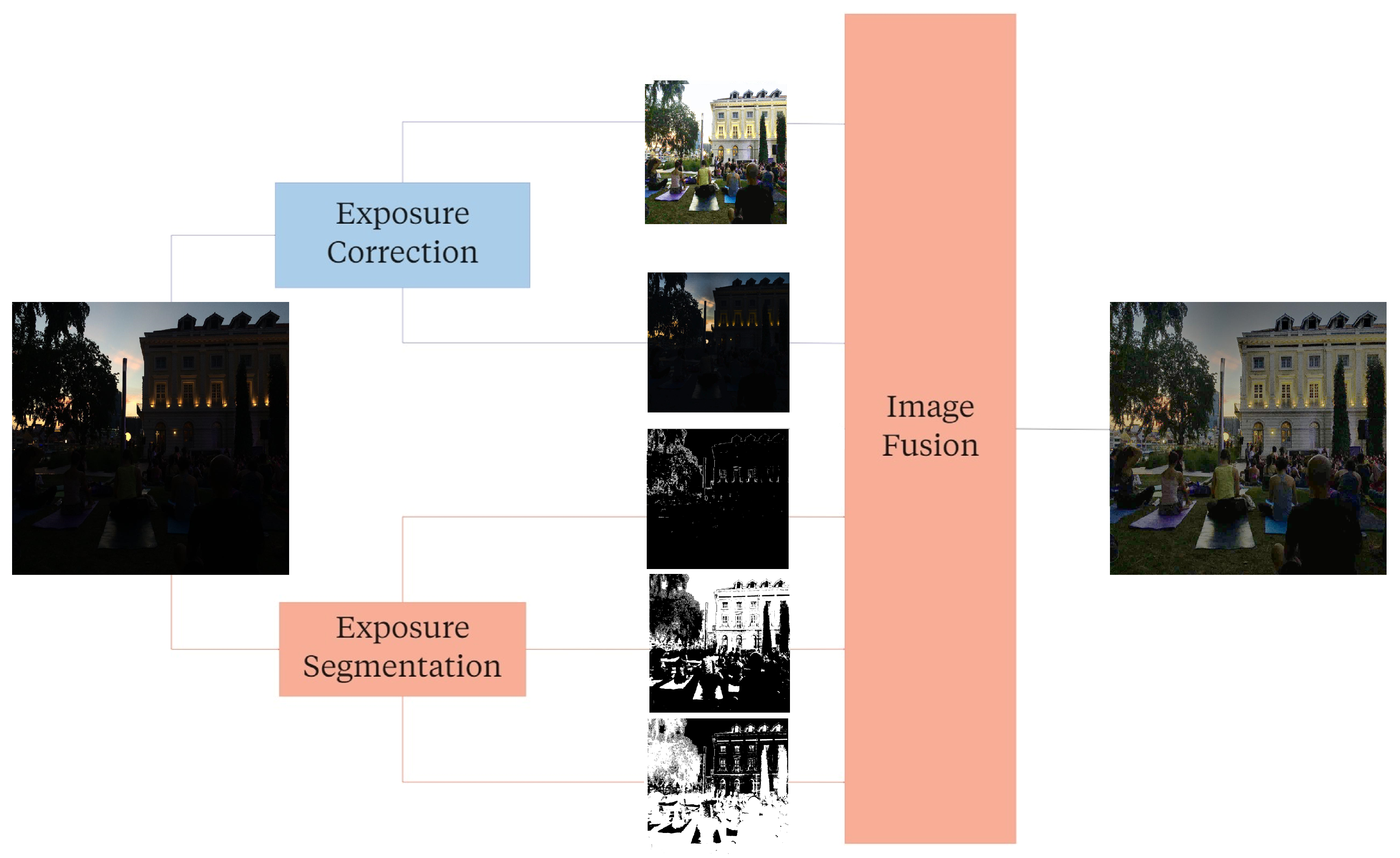
Figure 1, comprises three main modules, each playing a specific role in improving the quality of the final image. We designed the first two, Exposure Correction (EC) and Exposure Segmentation (ES), to work in parallel. Simultaneously advancing the flow enabled us to boost all the steps required to reach the final module. EC aims to adjust the exposure of acquired images to an optimal level, using a DL method that automatically adapts to different lighting conditions. The isolation of Regions Of Interest (ROIs) based on their exposure levels is achieved by ES through the application of IP techniques such as global thresholding and edge detection. ES allows the system to process each ROI independently, ensuring that the final image contains only the information of interest. Finally, the last module, Image Fusion (IF), combines both EC and ES results to produce the final outcome. IF takes as input the information of all ROIs and corrections collected from the previous stages and fuses them to create a single image with an optimal exposure level.
2.1.1. Exposure Correction (EC)
The EC module adjusts the brightness and contrast of an image to achieve an optimal level of visibility and detail. In recent years, researchers have proposed several DL methods for exposure adjustments and demonstrated their effectiveness in several applications, including surveillance, robotics, and photography [
22,
23,
24,
25].
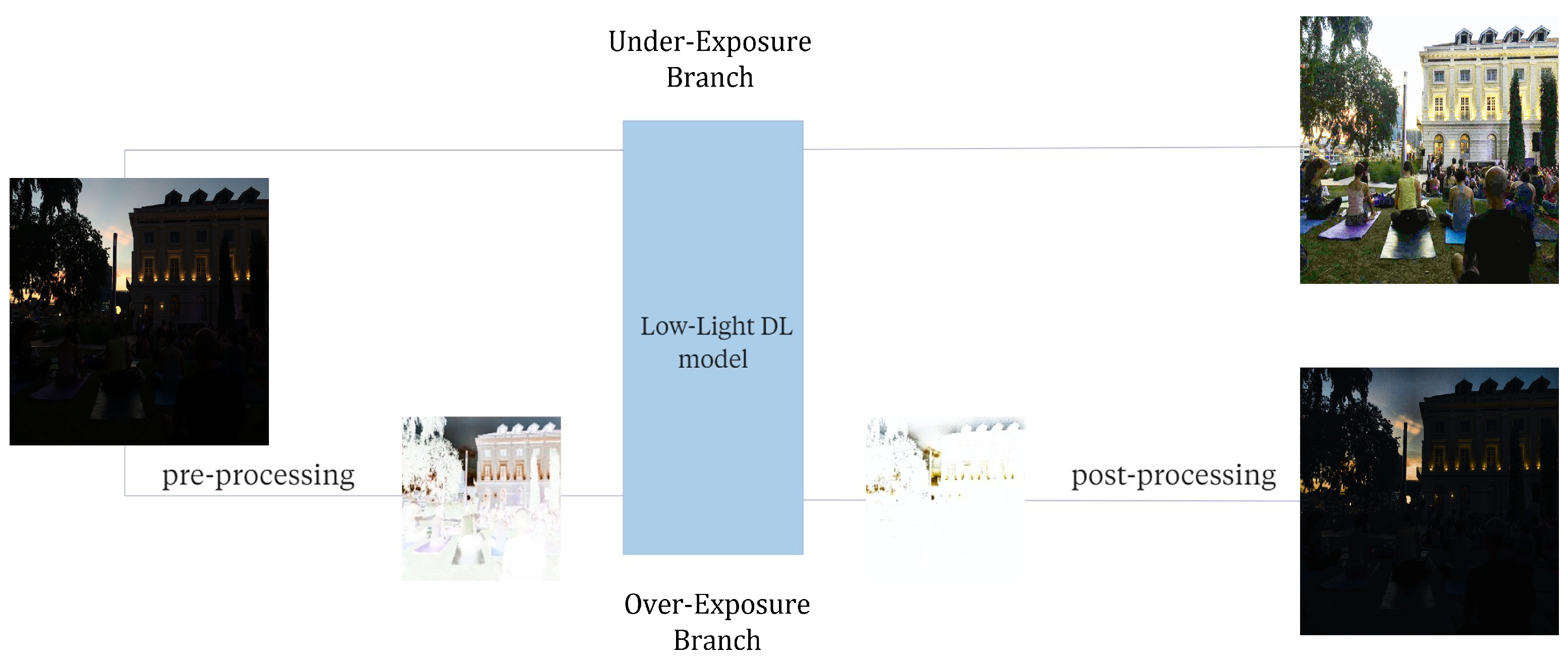
In the following section, we describe the DL framework for exposure adjustment in rescue scenarios. We subdivide it into two parallel branches, namely the Under-Exposure Branch (
) and the Over-Exposure Branch (
), which perform the under- and overexposure corrections, respectively. Both share the same unsupervised DL model designed for low-light image enhancement. In the
, we apply the model directly to the original images to correct and recover their dark areas. Instead, for the
, we introduce a pre-processing step on the original images to treat the overexposure correction as if it were an underexposure recovery problem. After the application of the model, at the end of
, a post-processing step is necessary to restore the original appearance of the images. Further details on the processing procedures are given at the end of this section. The high-level architecture of the EC module is outlined in
Figure 2.
Further details about the main components of EC are provided below:
Low-Light DL model: As DL model, we used the SCI (Self-Calibrated Illumination) [
8]. The model is designed to be fast and flexible, thus making it ideal for real-time situations with unpredictable lighting conditions, such as those encountered in rescue scenarios. To train the model, we selected low-light images from several publicly available datasets, including LOL DATASET [
6], Ex-Dark DATASET [
26], MIT-Adobe FiveK [
27]. This heterogeneous nature of the resulting data set was crucial to ensure that the training data set was diverse and representative of a wide range of low-light scenarios.
The resulting training dataset comprises 2500 images captured under different indoor and outdoor lighting conditions, thus ranging from high-quality images with good resolution and minimal noise to very noisy ones with low visibility. The dataset features various scenes and subjects, including landscapes, indoor scenes, and objects, thus providing a varied set of low-light scenarios. Diversity was further increased through data augmentation techniques such as rotation, flipping, and cropping, which create additional images and improve the model’s ability to generalise to different scenarios.
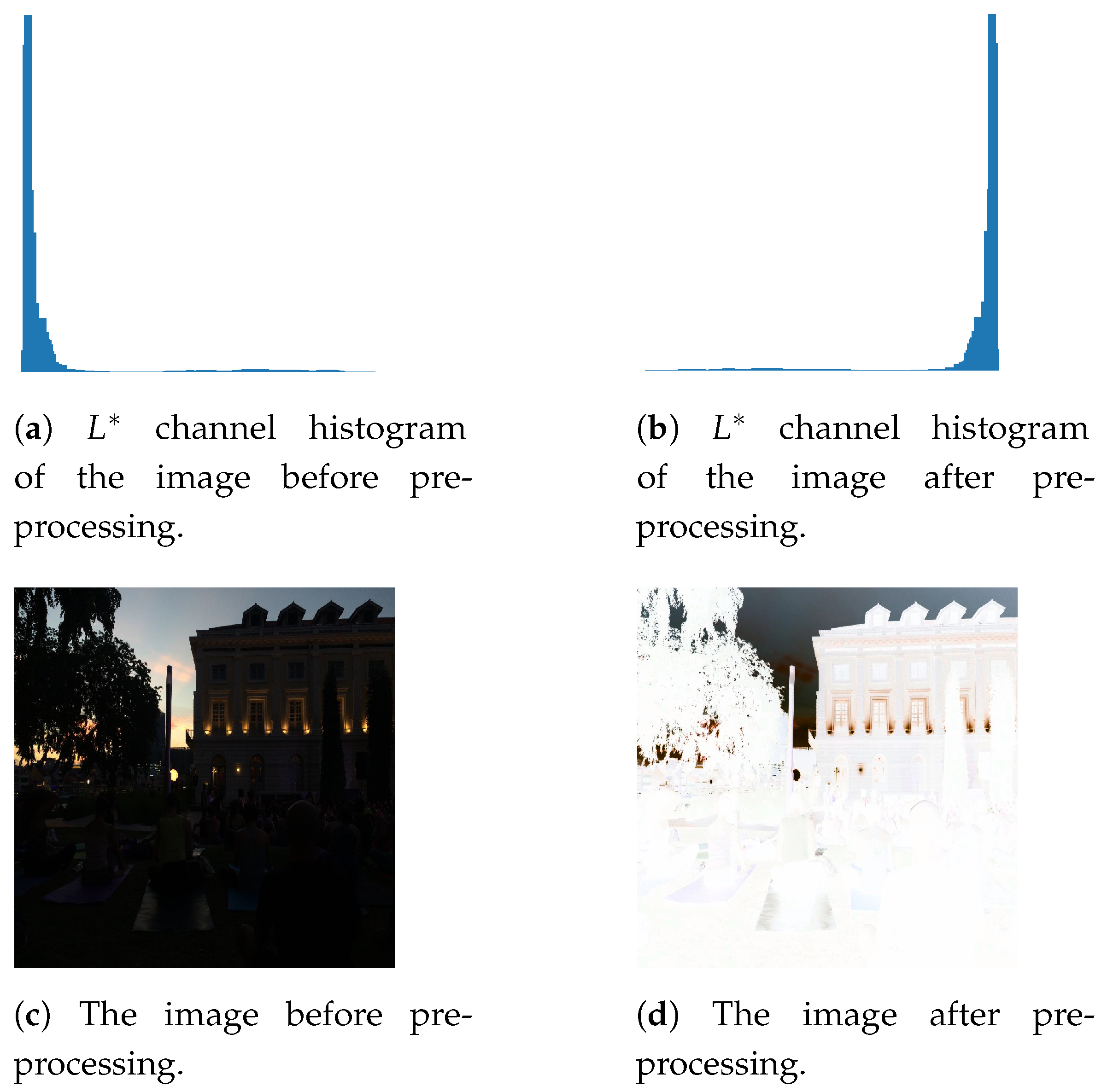
processing: To perform the overexposure correction, we first pre-process the input exploiting the CIELAB color space since it separates colour information (encoded in the
and
channels) from lightness information (encoded in the
channel). Independent manipulation of the
channel has been valuable in reversing brightness without affecting the colour appearance of the original images. In addition, CIELAB is designed to be perceptually uniform, which means that equal changes in lightness should appear to be equally perceptible. Therefore, inverting the
channel results in negated images, with the relative differences between the lightness values of different colours remaining consistent. This pre-processed image is then fed to the
(see
Figure 3). Once the model is applied, we post-process the image by reversing the
channel to recover its original lighting distribution.
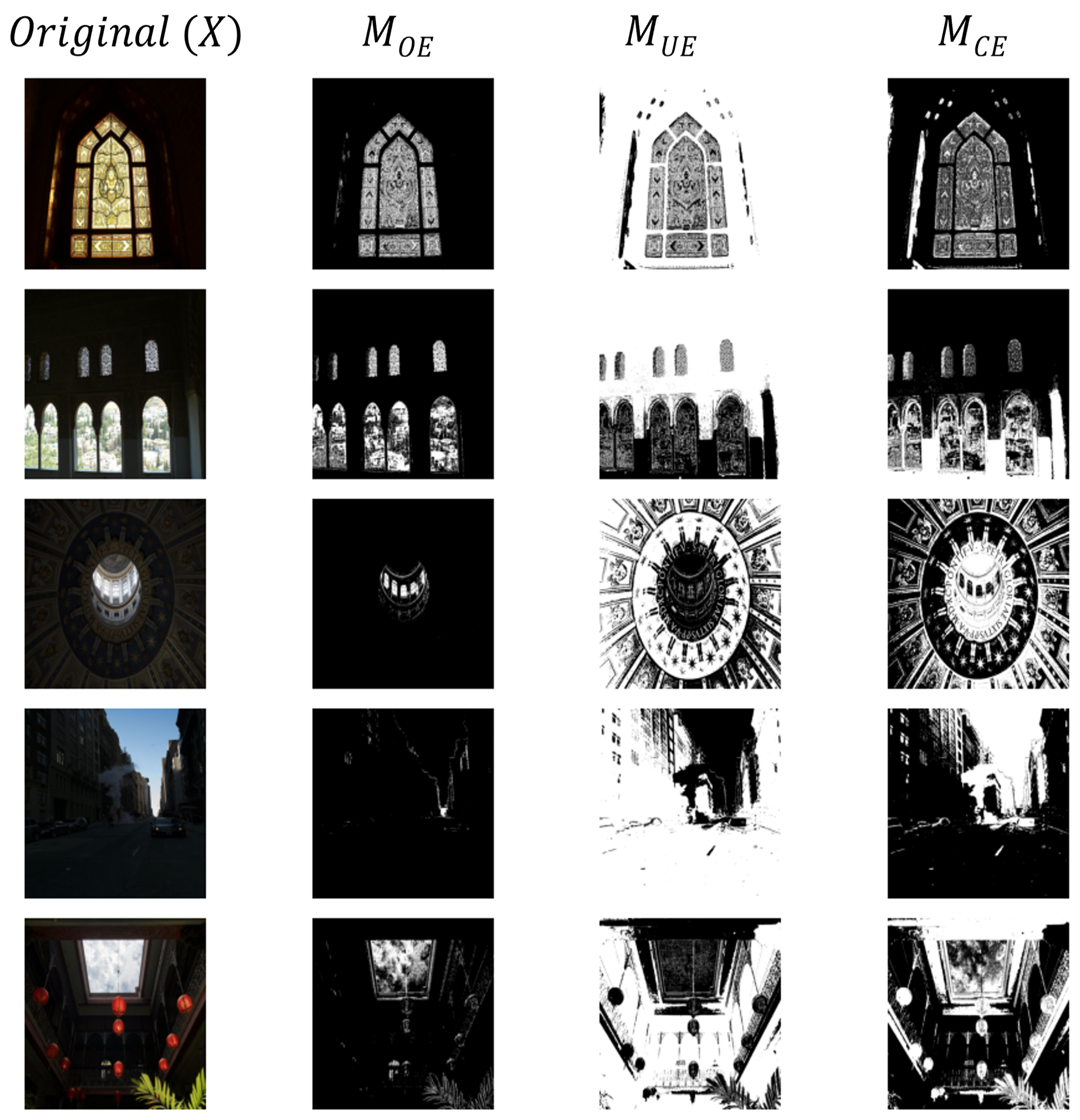
2.1.2. Exposure Segmentation (ES)
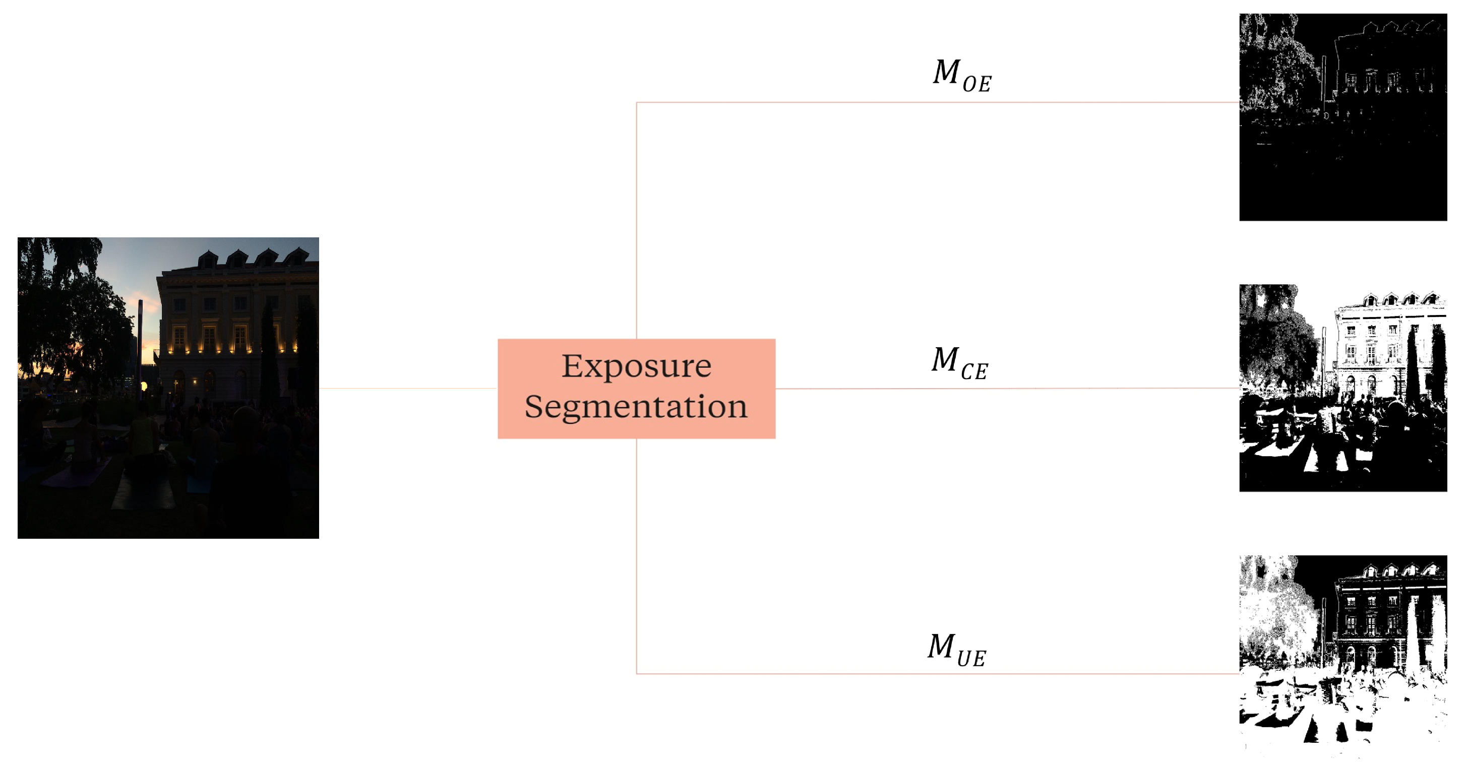
EC outputs complementary results, which need to be merged based on the exposure conditions of the original image. The ES module identifies the overexposed or underexposed regions of the original image, thus allowing the construction of a final image with a more balanced exposure and a wider range of details. Specifically, the module outputs three binary images (
,
, and
), which refer to the Over, Under, and Correctly-Exposed Masks, respectively (see
Figure 4).
We created the segmentation masks using lightness, saturation, and contrast information, as detailed in Equations (
1)–(
5). The first two components are retrieved from the HSV (Hue, Saturation, Value) color space, which separates the chromatic (H and S) from the lightness information (V). The Contrast (C) information is obtained by taking the absolute value of the Laplacian of the grayscale version of the images and then applying a threshold to the resulting Laplacian image. This thresholding step helps suppress low-amplitude noise and retain only the most prominent features, resulting in the thresholded version of C, denoted as
.
The three visual attributes that contribute to mask generation are determined by the properties of the regions being segmented. Overexposed regions occur when too much light enters the camera, resulting in washed-out or overly bright images that appear white and blown out. Conversely, underexposure happens when too little light enters the camera, resulting in dark images with less vibrant colours.
Masks were obtained using the following thresholding relationships:
where
,
, and
are the Over-Exposed, Under-Exposed, and Correctly-Exposed Masks.
V and
S are the Value and the Saturation channels of the HSV version of the image scaled between
. To include edges and textures information, for each mask
, we applied:
where
is the following binary mask:
The selection of threshold values for the over- and underexposed masks was guided by both empirical observation and domain knowledge, the latter being derived from a literature review of typical brightness and saturation ranges for such regions. This knowledge allowed us to narrow the range of values to test empirically and helped us select threshold values that were more likely to capture the relevant characteristics of the image [
28,
29,
30,
31,
32].
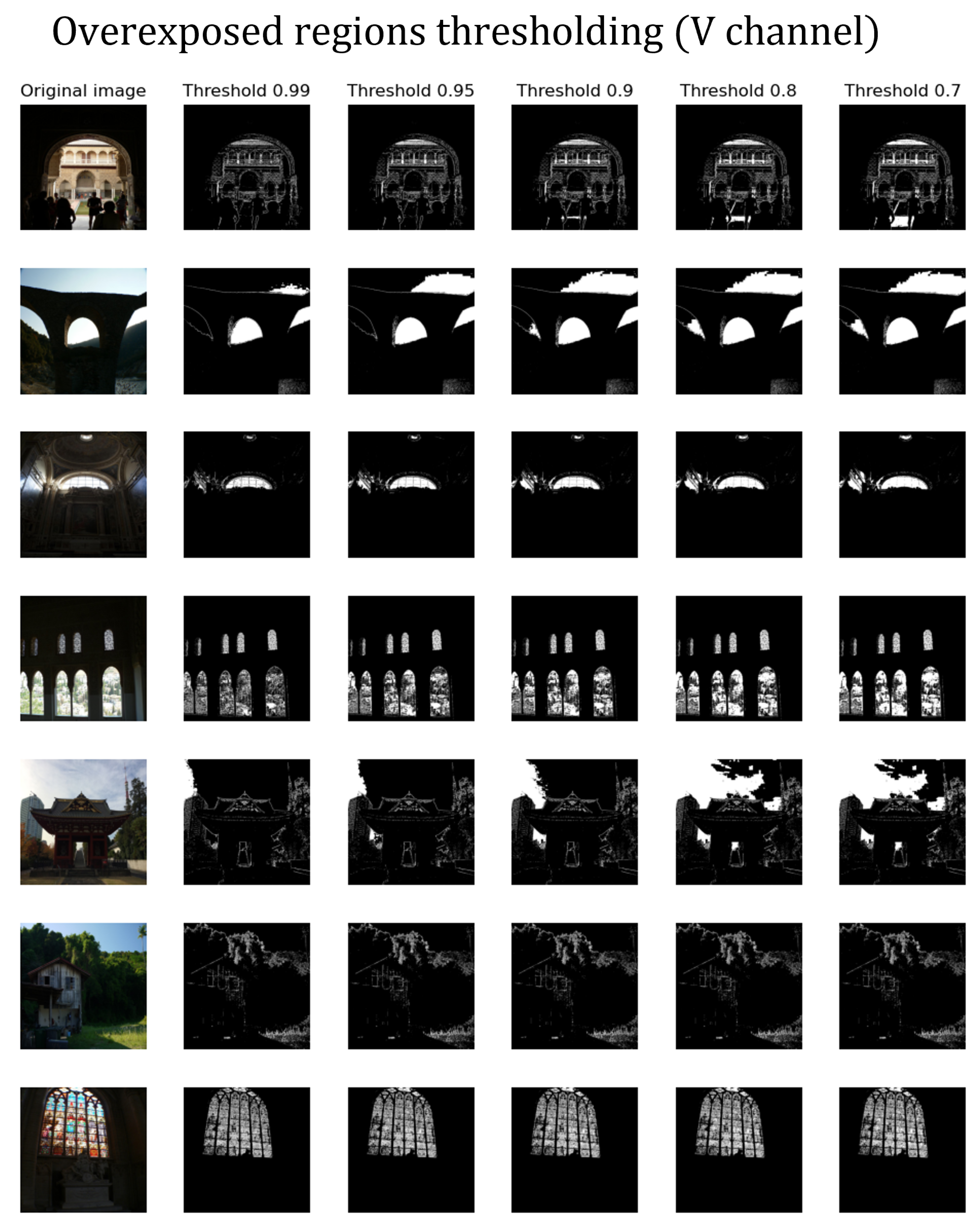
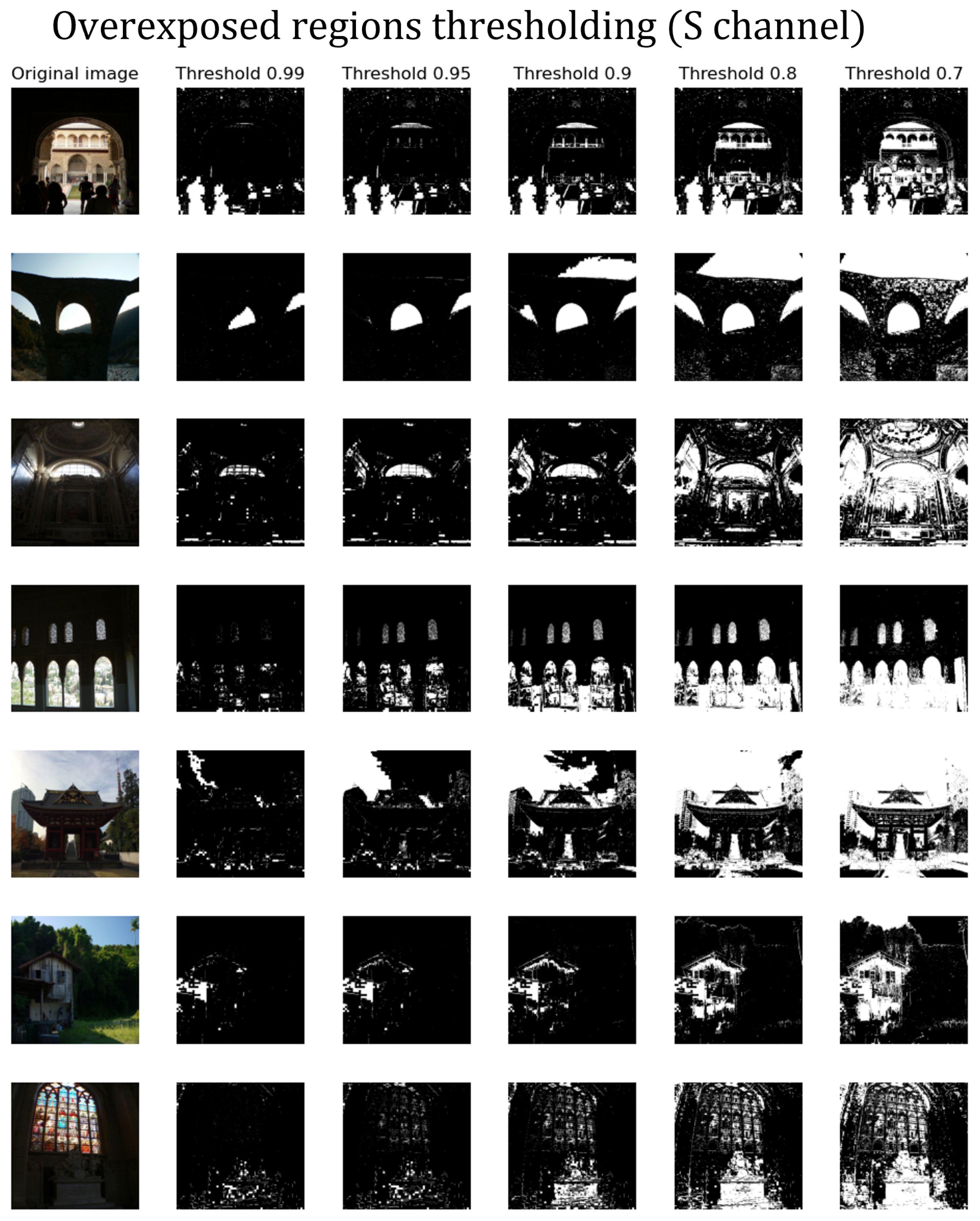
We experimentally tested various threshold values to determine the optimal ones and visually evaluated the resulting masks to assess their accuracy in identifying over- and underexposed regions. Based on this evaluation, we found that a threshold value of 0.9 for brightness and 0.1 for saturation was effective in detecting overexposed regions, while a threshold value of 0.1 for brightness was effective in identifying underexposed regions. Examples of masks generated using different thresholds are presented in
Appendix A.
Figure 5 highlights some results of the ES module.
2.1.3. Image Fusion (IF)
In the final stage of the pipeline, the intermediate results are merged to produce the final, corrected image. The module takes the original image (
X) and the intermediate correction results, namely
for the
correction and
for the
correction, along with their respective non-overlapping masks (
,
, and
) as input. The merging process, as introduced in [
33], relies upon a Hadamard product (denoted by the symbol ∘) to combine the input images and their corresponding masks:
The formula ensures that the final image is a combination of the correctly exposed regions of the original image and the regions corrected by the and branches, as defined by their respective masks. This property is guaranteed by the fact that the three masks (, , and ) are mutually exclusive and together form a matrix of ones, except for the edges.
Although Equation (
6) ensures that the resulting image covers all the desired regions, it may produce abrupt transitions and visible artefacts. Therefore, to produce a final image with smooth transitions between regions and a natural-looking appearance, we utilise the Laplacian Pyramid Blending [
34], which involves the following steps:
Pyramid Creation: Construction of the Laplacian Pyramids of X, and , as well as the Gaussian Pyramids of , and .
Layer Fusion: Apply Equation (
6) layer-wise to the pyramids generated in the previous step to obtain the Pyramid of Blended images (
).
Reconstruction: Reconstruct the final image from by performing the following steps: at each level, expand the current layer with lower resolution to match the size of the next level in the pyramid. Add the expanded layer to the corresponding layer in the pyramid to form a higher-resolution blended image. Repeat this process until the final level is reached, yielding the final blended image with the original resolution.
3. Results
In this section, we report on the results of the pipeline and show that it meets the requirements for rescue scenarios. To do so, we evaluate its performance in terms of details recovery, object detection improvement, and efficiency.
As stated in
Section 1, we measure the effectiveness of our method on the data set collected at the Weeze earthquake pilot. Our dataset comprises 282 images that depict earthquake scenarios, taken both indoors and outdoors. The images are available in both RAW and JPG formats and have a resolution of 3840 × 5750 pixels. They were captured in a variety of exposure settings, mostly featuring buildings and humans in the scenes.
3.1. Details Recovery
A crucial aspect of the pipeline is enhancing images through heightened detail, but the subjective nature of image quality poses a challenge in demonstrating improvements. To address this issue, we analysed several aspects of our results.
Reference-based Image Quality Analysis: In this section, we evaluate the quality of the images produced by the pipeline by comparing them with reference images (R). R is obtained by using Automatic Exposure Bracketing (AEB) [
35], a technique that captures the same scene several times at different exposure levels.
To quantify the similarity between the reference images and the pipeline’s outputs, we utilise two widely used image quality metrics: Mean Squared Error (MSE) and Structural Similarity Index (SSIM) [
36]. Both metrics are computed for both the original and the output images with respect to the reference images. MSE computes the average of the squared differences between the pixel intensities of two images, while SSIM compares the structural information and texture of the images to provide a measure of similarity. By deriving both metrics for the original images and the pipeline’s outputs, we determine whether the pipeline outputs are more similar to the reference images than the original ones. The average MSE and SSIM for both sets of images are presented in
Table 1. In addition to reporting the average MSE and SSIM for the original and output images, we analysed the distribution of these metrics across all images used in our evaluation. In
Appendix B, we use box plots to visualise the distribution of the MSE and SSIM values for both sets of images (
Figure A4); we also display a sample of the images along with their corresponding MSE and SSIM values in
Table A1 and
Table A2.
Image Characteristics Evaluation: The image characteristics of both original images and pipeline results were assessed using a set of metrics, including Texture (T), Entropy (E), Object Count (OC), Segmentation Masks (SM), and Hue Similarity Index (HSI).
T (Texture): Measures the visual pattern or structure of the images. We compute it by getting the variance of random images’ windows.
E (Shannon Entropy): Measures the degree of disorder in the images. A higher value indicates that the image has more information content, whereas a lower value indicates that the image has less degree of uncertainty. The comparison of Shannon entropy [
37] of
X and
Y quantifies the changes in information content resulting from the correction process.
OC (Object Count): OC represents the number of objects in an image. We obtain the metric by counting the connected components of the images. In particular, a connected component is defined as a set of pixels in the image that are connected through a path of neighbouring pixels of similar intensities.
Table 2 displays the values of the three metrics mentioned above, calculated for both the original and corrected images. To reduce any noise that may have been introduced during the exposure correction process, we applied an average smoothing filter to the images. Taking this step ensures that the metrics reflect the amount of detail recovered from the corrected images.
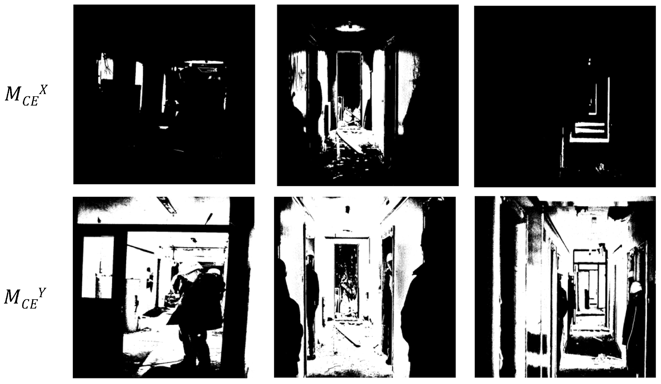
SM (Segmentation Masks): Segmentation masks are used to identify different regions or objects within an image. In particular, we used the mask
to identify well-exposed areas of the images before and after correction, as shown in
Figure 6.
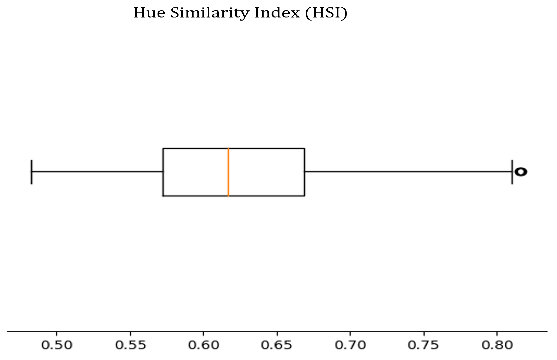
HSI (Hue Similarity Index): Hue Similarity Index is a metric used to measure the similarity between the hue values of the original and corrected images. We calculated HSI as the Pearson correlation coefficient [
38] on the Hue channel of the HSV version of the original and corrected images.
Figure 7 shows the box plot of the HSI values for the original and corrected hue channels. Our results demonstrate a linear relationship between the two pairs of images, indicating that our pipeline effectively preserves colour consistency.
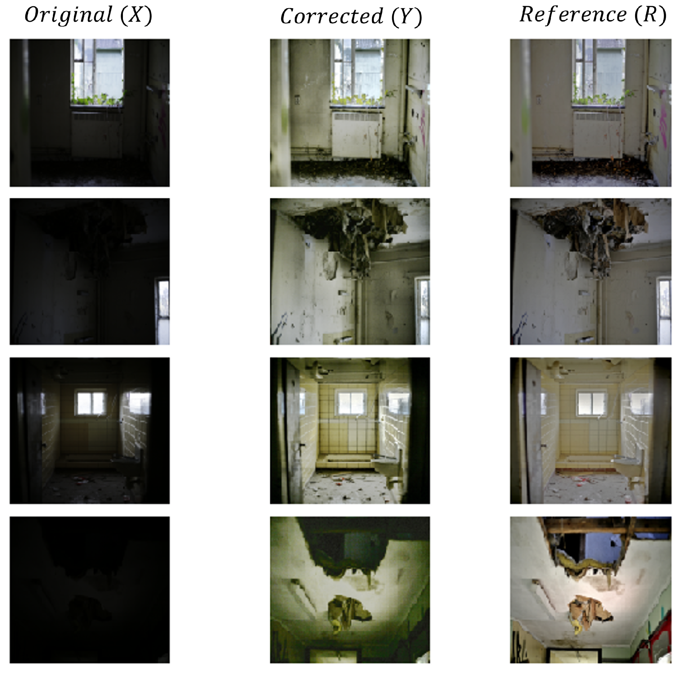
Visual Inspection: To demonstrate the effectiveness of our procedure, we compare the results (
Y) obtained by applying the pipeline to the initial images (
X) with the reference images (
R), as shown in
Figure 8.
3.2. Object Detection Improvement
In rescue scenarios, accurately locating and identifying individuals is critical. However, when a scene is not properly exposed, certain features of its objects can be obscured or washed out, making it difficult for the detector to identify them. To test and evaluate the pipeline’s effectiveness in identifying people, we used the YOLOv7 [
39] object detector, which is a state-of-the-art deep learning model for object detection. Specifically, we used the pre-trained weights of YOLOv7 on the Microsoft COCO: Common Objects in Context data set [
40], which contains a large number of annotated images of objects belonging to 80 different categories, including people. We applied the detector to both the original and corrected images, to assess its performance in identifying people under different lighting conditions.
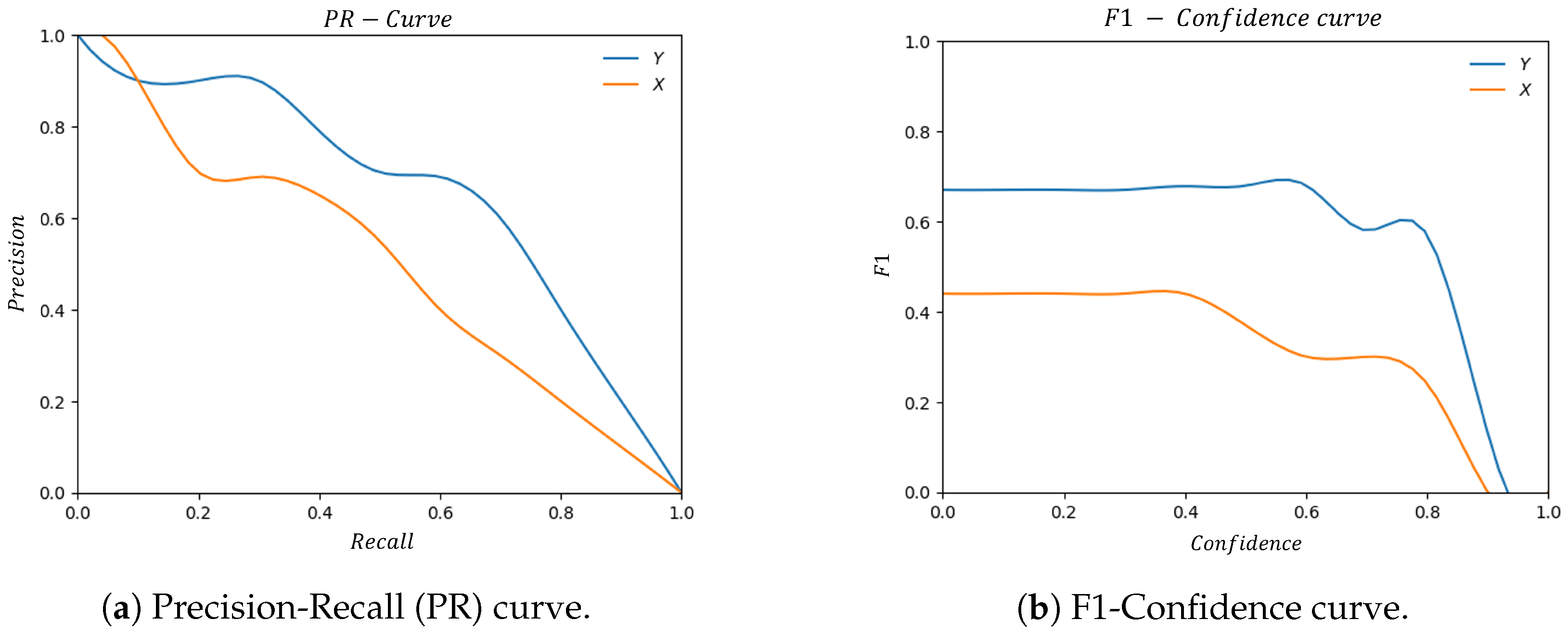
The detector performances were evaluated using: Precision (P), Recall (R), F1-score (F1), and Average Precision (AP). Precision computes the proportion of true positives (correctly detected people) among the total number of people detected. Recall is a measure of the proportion of true positives among the total number of actual people. F1-score is the harmonic mean of precision and recall. Average Precision (AP) evaluates the accuracy of the detector based on its precision and recall and it is calculated as the area under the Precision-Recall (PR) curve, which plots the precision values against the corresponding recall values at different detection thresholds.
The performances are summarised through the Precision-Recall (PR) and F1-Confidence curves shown in
Figure 9a,b. Additionally, the Average Precision (AP) is reported in
Table 3 to provide a comprehensive evaluation of our model’s performance. In
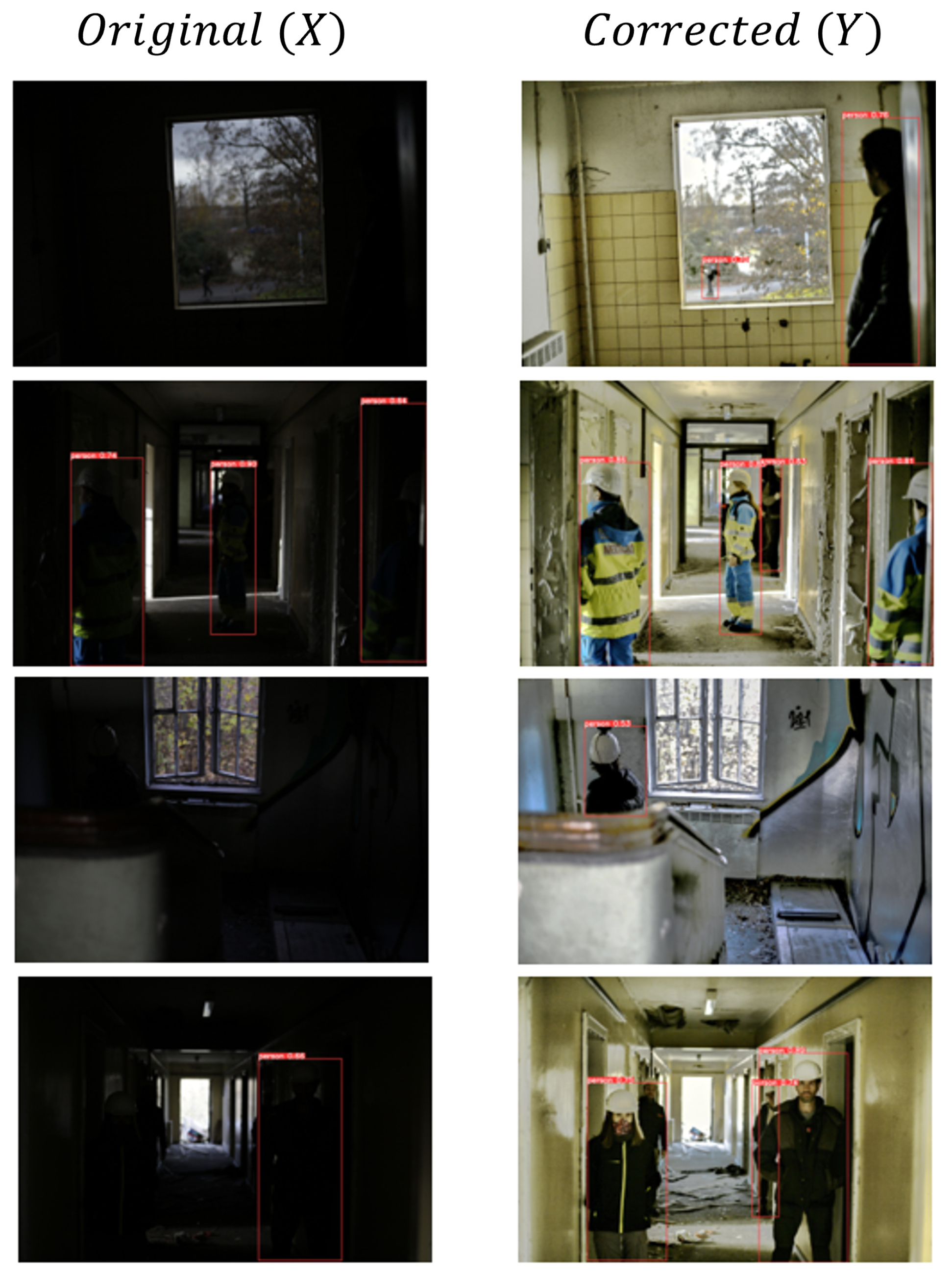
Figure 10, we also provide a visual comparison of the predicted bounding boxes.
3.3. Efficiency
Having fast corrections is of the utmost importance in real-time operational scenarios. Therefore, one of the requirements of the pipeline is that it has a response time suitable for rescue scenarios. To evaluate the pipeline efficiency, we first calculate the time needed to arrive at the IF module (1st stage) and then the time required for the fusion (2nd stage). Calculating the time of the 1st stage is a matter of computing the longest time between the parallel branches of the pipeline (see
Figure 11). In
Table 4, we report the running time (s) for images of different shapes (Width (W), Height (H), Channels (C)) by averaging 10,000 experiments conducted on an NVIDIA GeForce GTX 1650 using the CUDA toolkit version 11.7.
4. Discussion
The results of our pipeline indicate that it effectively meets the requirements for rescue scenarios. Our methodology was able to improve image detail, enhance object detection, and provide fast processing.
As described in the details recovery
Section 3.1, we used several metrics to evaluate the image characteristics of the pipeline’s outputs compared to the original images. The results showed that the pipeline was able to improve the complexity of the image’s texture, increase the information content, and augment the number of objects detected. Reference-based image quality analysis also demonstrated that the pipeline was able to produce images with higher quality compared to the original images, as evidenced by the reduced MSE and increased SSIM. Visual inspection further supported these results, providing a clear side-by-side comparison of the original, reference, and corrected images.
One of the main objectives of this model was to improve the light environment to boost the efficiency of other vision DL models, and this goal has been achieved as detailed in the object detection improvement
Section 3.2. The section highlighted how the pipeline was able to improve the performance of the YOLOv7 object detector in the detection of people. The results indicated that the corrected images allowed the model to identify individuals with higher Precision, Recall, F1-score, and Average Precision compared to the original images. The Precision-Recall and F1-Confidence curves, as well as the visual comparison of the predicted bounding boxes, provided clear evidence of the improvement in people detection.
The Efficiency
Section 3.3, indicates that the pipeline was able to process and provide information quickly enough to meet real-time requirements, which is essential in rescue scenarios. The results showed that the pipeline was able to reach the IF module (1st stage) and complete the fusion stage in a reasonable time even for images with different shapes.
5. Conclusions
In this study, we propose a pipeline of Deep Learning (DL) and Image-Processing (IP) techniques to improve the Situational Awareness (SA) of First Responders (FRs) in adverse lighting conditions. The pipeline consists of three modules: Exposure Correction (EC), Exposure Segmentation (ES), and Image Fusion (IF). EC aims to adjust the exposure of the acquired images to an optimal level, ES separates the images into regions of interest based on their exposure levels, and IF combines both the EC and ES results to produce the final image. The proposed method offers a solution to the challenges faced by FRs to enhance their operational capacity and allow them to make more informed decisions in high-pressure and fast-paced rescue scenarios.
While our method has shown improvements in image detail recovery, object detection performance, and fast processing, there is still room for improvement to address its limitations and expand its applicability. In particular, while our ES module strikes a balance between image enhancement and fast inference, we recognize that there is potential to explore adaptive thresholds or learning-based segmentation to improve its effectiveness in complex situations. Additionally, generating exposure segmentation masks with high precision is essential for ensuring the accuracy and reliability of our model.
To further enhance the performance and applicability of our method, we plan to modify the pipeline by removing its dependencies on the ES module. Specifically, we aim to use the EC module to generate multiple images with different exposure levels and merge them to create an image with a wider dynamic range. We intend to explore the integration of our pipeline into augmented reality visualization tools like the Hololens, which could offer new possibilities for real-world applications.
Through the Modane pilot, we plan to collaborate with professional first responders, including firefighters and medical rescuers, to gather feedback and refine it based on input from actual end-users.
In conclusion, the proposed pipeline provides a solution to the challenges faced by FRs under adverse lighting conditions, and the results indicate its potential for further development and implementation in real-world scenarios.
Author Contributions
Conceptualization, A.D.M. and I.A.; Formal analysis, A.D.M.; Funding acquisition, I.G.O.; Investigation, A.D.M., I.A. and X.O.B.; Methodology, A.D.M. and I.A.; Project administration, I.G.O.; Software, A.D.M.; Supervision, I.A., G.L. and I.G.O.; Validation, A.D.M., I.A. and X.O.B.; Writing—original draft, A.D.M.; Writing—review & editing, I.A., G.L. and I.G.O. All authors have read and agreed to the published version of the manuscript.
Funding
This research work was supported by the EU Horizon 2020 Grant Agreement no. 101021836 for the RESCUER (first RESponder-Centered support toolkit for operating in adverse and infrastrUcture-less EnviRonments) project.
https://cordis.europa.eu/project/id/101021836, accessed on 23 April 2021 (Project Link).
Institutional Review Board Statement
Not applicable.
Informed Consent Statement
Not applicable.
Data Availability Statement
Not applicable.
Acknowledgments
We are grateful to all the individuals who participated in the creation of the validation set at the WEEZE earthquake pilot. Their contributions were invaluable in making this research possible. A.D.M. acknowledges a traineeship grant from Vicomtech Foundation.
Conflicts of Interest
The authors declare no conflict of interest.
Abbreviations
The following abbreviations are used in this manuscript:
| DL | Deep Learning |
| IP | Image-Processing |
| FRs | First Responders |
| SA | Situational Awareness |
| AI | Artificial Intelligence |
| HDR | High Dynamic Range |
| LDR | Low Dynamic Range |
| IA | Intelligence Amplification |
| EC | Exposure Correction |
| ES | Exposure Segmentation |
| ROI | Regions of Interest |
| IF | Image Fusion |
|
| Under-Exposure Branch |
|
| Over-Exposure Branch |
|
| Over-Exposed Mask |
|
| Under-Exposed Mask |
|
| Correctly-Exposed Mask |
|
| Pyramid of Blended images |
| MSE | Mean Squared Error |
| SSIM | Structural Similarity Index |
| AEB | Automatic Exposure Bracketing |
| R | Reference images |
| T | Texture |
| E | Entropy |
| OC | Object Count |
| SM | Segmentation Mask |
| P | Precision |
| R | Recall |
| F1 | F1-score |
| AUC | Area Under the Curve |
| AP | Average Precision |
Appendix A
Here we provide an overview of the experimental setup and methodology used to generate the masks discussed in
Section 2.1.2. The aim of these experiments was to determine optimal threshold values to detect over- and underexposed regions in images, based on a combination of empirical observation and domain knowledge. To begin, we conducted a thorough literature review of typical brightness and saturation ranges for over- and underexposed regions in images, which allowed us to narrow down the range of values to test empirically. We then systematically tested various threshold values for brightness and saturation, visually evaluating the resulting masks to determine their accuracy in identifying over- and underexposed regions.
Figure A1,
Figure A2 and
Figure A3 represent the experiments.
Figure A1.
Threshold adjustment. This figure showcases experiments conducted on the V channel of the HSV version of original images to determine the optimal threshold values for generating masks.
Figure A1.
Threshold adjustment. This figure showcases experiments conducted on the V channel of the HSV version of original images to determine the optimal threshold values for generating masks.
Figure A2.
Threshold adjustment. This figure showcases experiments conducted on the V channel of the HSV version of original images to determine the threshold values for generating masks.
Figure A2.
Threshold adjustment. This figure showcases experiments conducted on the V channel of the HSV version of original images to determine the threshold values for generating masks.
Figure A3.
Threshold adjustment. This figure presents experiments conducted on the S channel of the HSV version of the original images to determine the threshold values for generating masks.
Figure A3.
Threshold adjustment. This figure presents experiments conducted on the S channel of the HSV version of the original images to determine the threshold values for generating masks.
Appendix B
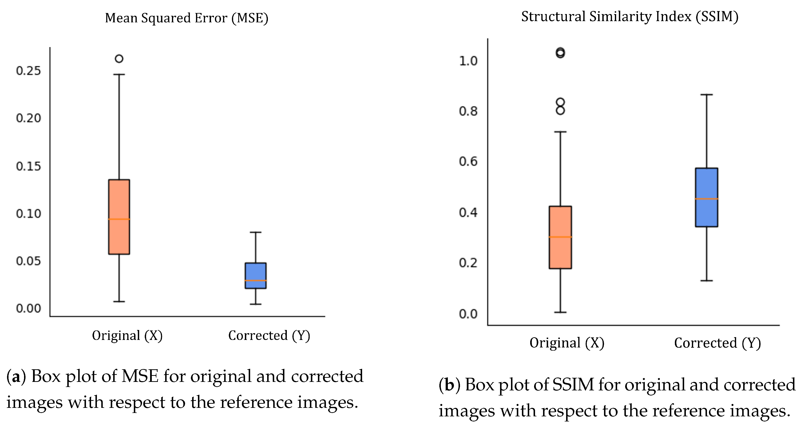
Here, we present supplementary information regarding the outcomes of our methodology. Specifically, we include box plots that illustrate the mean squared error (MSE) and structural similarity index measure (SSIM) of both the original and corrected images in comparison to the reference images, as depicted in
Figure A4. Additionally, we offer two tables containing the MSE and SSIM values of a randomly selected subset of 20 images each.
Table A1 represents a sample of MSE for the original and corrected images compared to the reference images. The MSE values demonstrate the accuracy of the images before and after correction, with lower values indicating better results.
Similarly,
Table A2 shows a sample of the SSIM values for both the original and corrected images with respect to the reference images. SSIM values measure the structural similarity between images and are used to evaluate the quality of corrected images. Higher SSIM values indicate better similarity between images.
Figure A4.
(a) shows the box plot of Mean Squared Error (MSE) between the original and reference images and between the corrected and reference images. (b) shows the Structural Similarity Index (SSIM) box plot between the original and reference images, and between the corrected and reference images.
Table A1.
Mean Squared Error (MSE) values for a sample of the images.
Table A1.
Mean Squared Error (MSE) values for a sample of the images.
| Original (X) | Corrected (Y) |
|---|
| 0.089 | 0.027 |
| 0.119 | 0.038 |
| 0.150 | 0.018 |
| 0.098 | 0.013 |
| 0.099 | 0.057 |
| 0.012 | 0.010 |
| 0.028 | 0.027 |
| 0.176 | 0.031 |
| 0.098 | 0.007 |
| 0.087 | 0.026 |
| 0.076 | 0.018 |
| 0.043 | 0.028 |
| 0.140 | 0.039 |
| 0.135 | 0.052 |
| 0.130 | 0.065 |
| 0.223 | 0.047 |
| 0.044 | 0.049 |
| 0.065 | 0.050 |
| 0.142 | 0.024 |
| 0.011 | 0.035 |
Table A2.
Structural Similarity Index (SSIM) values for a sample of the images.
Table A2.
Structural Similarity Index (SSIM) values for a sample of the images.
| Original (X) | Corrected (Y) |
|---|
| 0.441 | 0.444 |
| 0.303 | 0.694 |
| 0.247 | 0.463 |
| 0.140 | 0.564 |
| 0.003 | 0.199 |
| 0.441 | 0.801 |
| 0.562 | 0.442 |
| 0.509 | 0.572 |
| 0.717 | 0.652 |
| 0.035 | 0.588 |
| 0.338 | 0.781 |
| 0.392 | 0.582 |
| 0.683 | 0.699 |
| 0.611 | 0.640 |
| 0.358 | 0.486 |
| 0.369 | 0.373 |
| 0.358 | 0.462 |
| 0.111 | 0.131 |
| 0.103 | 0.597 |
| 0.302 | 0.206 |
References
- Singh, K.; Kapoor, R.; Sinha, S.K. Enhancement of low exposure images via recursive histogram equalization algorithms. Optik 2015, 126, 2619–2625. [Google Scholar] [CrossRef]
- Celik, T.; Tjahjadi, T. Contextual and variational contrast enhancement. IEEE Trans. Image Process. 2011, 20, 3431–3441. [Google Scholar] [CrossRef] [PubMed]
- Bhandari, A.K.; Subramani, B.; Veluchamy, M. Multi-exposure optimized contrast and brightness balance color image enhancement. Digit. Signal Process. 2022, 123, 103406. [Google Scholar] [CrossRef]
- Goyal, V.; Shukla, A. An enhancement of underwater images based on contrast restricted adaptive histogram equalization for image enhancement. In Smart Innovations in Communication and Computational Sciences: Proceedings of ICSICCS 2020; Springer: Singapore, 2021; pp. 275–285. [Google Scholar]
- Land, E.H. The retinex theory of color vision. Sci. Am. 1977, 237, 108–129. [Google Scholar] [CrossRef] [PubMed]
- Wei, C.; Wang, W.; Yang, W.; Liu, J. Deep retinex decomposition for low-light enhancement. arXiv 2018, arXiv:1808.04560. [Google Scholar]
- Liu, R.; Ma, L.; Zhang, J.; Fan, X.; Luo, Z. Retinex-inspired unrolling with cooperative prior architecture search for low-light image enhancement. In Proceedings of the IEEE/CVF Conference on Computer Vision and Pattern Recognition, Nashville, TN, USA, 20–25 June 2021; pp. 10561–10570. [Google Scholar]
- Ma, L.; Ma, T.; Liu, R.; Fan, X.; Luo, Z. Toward fast, flexible, and robust low-light image enhancement. In Proceedings of the IEEE/CVF Conference on Computer Vision and Pattern Recognition, New Orleans, LA, USA, 18–24 June 2022; pp. 5637–5646. [Google Scholar]
- Li, M.; Liu, J.; Yang, W.; Sun, X.; Guo, Z. Structure-revealing low-light image enhancement via robust retinex model. IEEE Trans. Image Process. 2018, 27, 2828–2841. [Google Scholar] [CrossRef]
- Wang, P.; Wang, Z.; Lv, D.; Zhang, C.; Wang, Y. Low illumination color image enhancement based on Gabor filtering and Retinex theory. Multimed. Tools Appl. 2021, 80, 17705–17719. [Google Scholar] [CrossRef]
- Pan, X.; Li, C.; Pan, Z.; Yan, J.; Tang, S.; Yin, X. Low-Light Image Enhancement Method Based on Retinex Theory by Improving Illumination Map. Appl. Sci. 2022, 12, 5257. [Google Scholar] [CrossRef]
- Mei, Y.; Qiu, G. Recovering high dynamic range radiance maps from photographs revisited: A simple and important fix. In Proceedings of the 2013 Seventh International Conference on Image and Graphics, Qingdao, China, 26–28 July 2013; pp. 23–28. [Google Scholar]
- Niu, Y.; Wu, J.; Liu, W.; Guo, W.; Lau, R.W. HDR-GAN: HDR image reconstruction from multi-exposed LDR images with large motions. IEEE Trans. Image Process. 2021, 30, 3885–3896. [Google Scholar] [CrossRef] [PubMed]
- Kalantari, N.K.; Ramamoorthi, R. Deep high dynamic range imaging of dynamic scenes. ACM Trans. Graph. 2017, 36, 144. [Google Scholar] [CrossRef]
- Mertens, T.; Kautz, J.; Van Reeth, F. Exposure fusion. In Proceedings of the 15th Pacific Conference on Computer Graphics and Applications (PG’07), Maui, HI, USA, 29 October–1 November 2007; pp. 382–390. [Google Scholar]
- Liu, Y.L.; Lai, W.S.; Chen, Y.S.; Kao, Y.L.; Yang, M.H.; Chuang, Y.Y.; Huang, J.B. Single-image HDR reconstruction by learning to reverse the camera pipeline. In Proceedings of the IEEE/CVF Conference on Computer Vision and Pattern Recognition, Seattle, WA, USA, 13–19 June 2020; pp. 1651–1660. [Google Scholar]
- Santos, M.S.; Ren, T.I.; Kalantari, N.K. Single image HDR reconstruction using a CNN with masked features and perceptual loss. arXiv 2020, arXiv:2005.07335. [Google Scholar] [CrossRef]
- Eilertsen, G.; Kronander, J.; Denes, G.; Mantiuk, R.K.; Unger, J. HDR image reconstruction from a single exposure using deep CNNs. ACM Trans. Graph. (TOG) 2017, 36, 1–15. [Google Scholar] [CrossRef]
- Raipurkar, P.; Pal, R.; Raman, S. HDR-cGAN: Single LDR to HDR image translation using conditional GAN. In Proceedings of the Twelfth Indian Conference on Computer Vision, Graphics and Image Processing, Jodhpur, India, 19–22 December 2021; pp. 1–9. [Google Scholar]
- Li, J.; Fang, P. Hdrnet: Single-image-based hdr reconstruction using channel attention cnn. In Proceedings of the 2019 4th International Conference on Multimedia Systems and Signal Processing, Guangzhou China, 10–12 May 2019; pp. 119–124. [Google Scholar]
- Vonikakis, V. Tm-Died: The Most Difficult Image Enhancement Dataset. Available online: https://sites.google.com/site/vonikakis/datasets (accessed on 15 December 2022).
- Lin, G.S.; Ji, X.W. Video quality enhancement based on visual attention model and multi-level exposure correction. Multimed. Tools Appl. 2016, 75, 9903–9925. [Google Scholar] [CrossRef]
- Steffens, C.; Drews, P.L.J.; Botelho, S.S. Deep learning based exposure correction for image exposure correction with application in computer vision for robotics. In Proceedings of the 2018 Latin American Robotic Symposium, 2018 Brazilian Symposium on Robotics (SBR) and 2018 Workshop on Robotics in Education (WRE), Joao Pessoa, Brazil, 6–10 November 2018; pp. 194–200. [Google Scholar]
- Afifi, M.; Derpanis, K.G.; Ommer, B.; Brown, M.S. Learning multi-scale photo exposure correction. In Proceedings of the IEEE/CVF Conference on Computer Vision and Pattern Recognition, Nashville, TN, USA, 20–25 June 2021; pp. 9157–9167. [Google Scholar]
- Jatzkowski, I.; Wilke, D.; Maurer, M. A deep-learning approach for the detection of overexposure in automotive camera images. In Proceedings of the 2018 21St international conference on intelligent transportation systems (ITSC), Maui, HI, USA, 4–7 November 2018; pp. 2030–2035. [Google Scholar]
- Loh, Y.P.; Chan, C.S. Getting to know low-light images with the exclusively dark dataset. Comput. Vis. Image Underst. 2019, 178, 30–42. [Google Scholar] [CrossRef]
- Bychkovsky, V.; Paris, S.; Chan, E.; Durand, F. Learning Photographic Global Tonal Adjustment with a Database of Input/Output Image Pairs. In Proceedings of the Twenty-Fourth IEEE Conference on Computer Vision and Pattern Recognition, Colorado Springs, CO, USA, 20–25 June 2011. [Google Scholar]
- Agarwal, S.; Agarwal, D. Histogram Equalization for Contrast Enhancement of both Overexposed and Underexposed Gray Scale Images. Adv. Comput. Control. Commun. Technol. 2016, 1, 1. [Google Scholar]
- Morgand, A.; Tamaazousti, M. Generic and real-time detection of specular reflections in images. In Proceedings of the 2014 International Conference on Computer Vision Theory and Applications (VISAPP), Lisbon, Portugal, 5–8 January 2014; Volume 1, pp. 274–282. [Google Scholar]
- Ortiz, F.; Torres, F. A new inpainting method for highlights elimination by colour morphology. In Proceedings of the Pattern Recognition and Image Analysis: Third International Conference on Advances in Pattern Recognition, ICAPR 2005, Bath, UK, 22–25 August 2005; Proceedings, Part II 3. Springer: Berlin/Heidelberg, Germany, 2005; pp. 368–376. [Google Scholar]
- Androutsos, D.; Plataniotis, K.N.; Venetsanopoulos, A.N. A novel vector-based approach to color image retrieval using a vector angular-based distance measure. Comput. Vis. Image Underst. 1999, 75, 46–58. [Google Scholar] [CrossRef]
- Guo, D.; Cheng, Y.; Zhuo, S.; Sim, T. Correcting over-exposure in photographs. In Proceedings of the 2010 IEEE Computer Society Conference on Computer Vision and Pattern Recognition, San Francisco, CA, USA, 13–18 June 2010; pp. 515–521. [Google Scholar]
- Szeliski, R. Image alignment and stitching: A tutorial. Found. Trends® Comput. Graph. Vis. 2007, 2, 1–104. [Google Scholar] [CrossRef]
- Burt, P.J.; Adelson, E.H. The Laplacian pyramid as a compact image code. In Readings in Computer Vision; Elsevier: Amsterdam, The Netherlands, 1987; pp. 671–679. [Google Scholar]
- Pourreza-Shahri, R.; Kehtarnavaz, N. Exposure bracketing via automatic exposure selection. In Proceedings of the 2015 IEEE international conference on image processing (ICIP), Quebec City, QC, Canada, 27–30 September 2015; pp. 320–323. [Google Scholar]
- Wang, Z.; Bovik, A.C.; Sheikh, H.R.; Simoncelli, E.P. Image quality assessment: From error visibility to structural similarity. IEEE Trans. Image Process. 2004, 13, 600–612. [Google Scholar] [CrossRef]
- Shannon, C.E. A mathematical theory of communication. ACM SIGMOBILE Mob. Comput. Commun. Rev. 2001, 5, 3–55. [Google Scholar] [CrossRef]
- Cohen, I.; Huang, Y.; Chen, J.; Benesty, J.; Benesty, J.; Chen, J.; Huang, Y.; Cohen, I. Pearson correlation coefficient. Noise Reduct. Speech Process. 2009, 27, 1–4. [Google Scholar]
- Wang, C.Y.; Bochkovskiy, A.; Liao, H.Y.M. YOLOv7: Trainable bag-of-freebies sets new state-of-the-art for real-time object detectors. arXiv 2022, arXiv:2207.02696. [Google Scholar]
- Lin, T.Y.; Maire, M.; Belongie, S.; Hays, J.; Perona, P.; Ramanan, D.; Dollár, P.; Zitnick, C.L. Microsoft coco: Common objects in context. In Proceedings of the Computer Vision–ECCV 2014: 13th European Conference, Zurich, Switzerland, 6–12 September 2014; Proceedings, Part V 13. Springer: Cham, Switzerland, 2014; pp. 740–755. [Google Scholar]
Figure 1.
Pipeline overview. The figure represents the main flow of the pipeline. The modules corresponding to Image-Processing (IP) techniques are coloured orange, whereas the module with the Deep Learning (DL) framework is coloured blue.
Figure 1.
Pipeline overview. The figure represents the main flow of the pipeline. The modules corresponding to Image-Processing (IP) techniques are coloured orange, whereas the module with the Deep Learning (DL) framework is coloured blue.
Figure 2.
Exposure correction (EC). The figure illustrates the EC module, comprising two parallel branches. The upper branch, labelled as the Under-Exposure Branch (), displays the direct application of the Low-Light DL model to the original image. The second branch, identified as the Over-Exposure Branch (), exhibits the intermediate processing steps required for correction.
Figure 3.
input generation. The image on the left is the original, and the image on the right is after pre-processing. Above each image is the histogram distribution of their lightness () channel. The conversion from (c) to (d) enabled us to treat the overexposure correction as an underexposure recovery problem.
Figure 4.
Exposure segmentation (ES). The input is the image under the original lighting conditions. The outputs are three binary images (, and ), which represent the Over, Under and Correctly-Exposed Masks, respectively.
Figure 4.
Exposure segmentation (ES). The input is the image under the original lighting conditions. The outputs are three binary images (, and ), which represent the Over, Under and Correctly-Exposed Masks, respectively.
Figure 5.
Segmentation masks. The figure represents some examples of our segmentation.
Figure 5.
Segmentation masks. The figure represents some examples of our segmentation.
Figure 6.
Segmentation Masks (SM). The upper part represents the Correctly-Exposed Mask of the original images (). The lower part depicts the same mask on the pipeline results ().
Figure 6.
Segmentation Masks (SM). The upper part represents the Correctly-Exposed Mask of the original images (). The lower part depicts the same mask on the pipeline results ().
Figure 7.
The figure reports the box plot of the Hue Similarity Index (HSI) for the original and corrected hue channels.
Figure 7.
The figure reports the box plot of the Hue Similarity Index (HSI) for the original and corrected hue channels.
Figure 8.
Visual comparison. The illustration shows a comparison of the original image (X), the image produced by the pipeline (Y), and the benchmark image (R).
Figure 8.
Visual comparison. The illustration shows a comparison of the original image (X), the image produced by the pipeline (Y), and the benchmark image (R).
Figure 9.
(a,b) show that a greater Area Under the Curve (AUC) corresponds to the corrected images.
Figure 9.
(a,b) show that a greater Area Under the Curve (AUC) corresponds to the corrected images.
Figure 10.
People detector. The figure represents the predicted boxes on some of the original and output images.
Figure 10.
People detector. The figure represents the predicted boxes on some of the original and output images.
Figure 11.
Stages overview. The figure represents the stages of the total computing time.
Figure 11.
Stages overview. The figure represents the stages of the total computing time.
Table 1.
The table represents the average Mean Squared Error (MSE) and Structural Similarity Index (SSIM) for both the original images (X) and the corrected images (Y) with respect to their references (R).
Table 1.
The table represents the average Mean Squared Error (MSE) and Structural Similarity Index (SSIM) for both the original images (X) and the corrected images (Y) with respect to their references (R).
| | MSE | SSIM |
|---|
| Original (X) | 0.101 ± 0.051 | 0.331 ± 0.185 |
| Corrected (Y) | 0.033 ± 0.014 | 0.476 ± 0.130 |
Table 2.
Texture (T), Entropy (E), and Object Count (OC) table. The table represents the average metrics for both the original (X) and the output images (Y).
Table 2.
Texture (T), Entropy (E), and Object Count (OC) table. The table represents the average metrics for both the original (X) and the output images (Y).
| | T | E | OC |
|---|
| Original (X) | 0.011 ± 0.022 | 0.0013 ± 0.035 | ∼144 |
| Corrected (Y) | 0.141 ± 0.012 | 0.0215 ± 0.003 | ∼867 |
Table 3.
Average Precision. The table represents the Average Precision (AP) values for both the original (
X) and the corrected (
Y) images, calculated using the Precision-Recall (PR) curve displayed in
Figure 9a.
Table 3.
Average Precision. The table represents the Average Precision (AP) values for both the original (
X) and the corrected (
Y) images, calculated using the Precision-Recall (PR) curve displayed in
Figure 9a.
| | Average Precision (AP) |
|---|
| Original (X) | 0.501 |
| Corrected (Y) | 0.658 |
Table 4.
Computation time. The table represents the average running time for images of different shapes.
Table 4.
Computation time. The table represents the average running time for images of different shapes.
|
| 1st Stage (s) | 2nd Stage (s) | Total (s) |
|---|
| (128, 128, 3) | 0.0011 | 0.0015 | 0.0026 |
| (256, 256, 3) | 0.0014 | 0.0041 | 0.0055 |
| (512, 512, 3) | 0.0027 | 0.0238 | 0.0265 |
| (1024, 1024, 3) | 0.0125 | 0.1036 | 0.1161 |
| (2048, 2048, 3) | 0.0424 | 0.3975 | 0.4399 |
| Disclaimer/Publisher’s Note: The statements, opinions and data contained in all publications are solely those of the individual author(s) and contributor(s) and not of MDPI and/or the editor(s). MDPI and/or the editor(s) disclaim responsibility for any injury to people or property resulting from any ideas, methods, instructions or products referred to in the content. |
© 2023 by the authors. Licensee MDPI, Basel, Switzerland. This article is an open access article distributed under the terms and conditions of the Creative Commons Attribution (CC BY) license (https://creativecommons.org/licenses/by/4.0/).


 ,
, 


