A Framework for Frugal Supervised Learning with Incremental Neural Networks

Abstract

This study proposes an implementation of an incremental neural network (INN) that was initially designed for affective computing tasks. INNs are a family of machine learning algorithms that combine prototype-based classifiers with neural networks. They achieve state-of-the-art performance with less data than traditional approaches. In this research, we conduct an in-depth review of INN mechanisms and present a research-grade framework that enables the use of INNs on arbitrary data. We evaluated our implementation on two different datasets, including the AVEC2014 Challenge, which involved predicting depressive state from auditive and visual modalities. Our results are encouraging, demonstrating the potential of INNs in situations where approaches have to be explainable or when data are scarce.

1. Introduction

The goal of this section is to provide a comprehensive review of the literature on prototype-based neural networks and to outline the motivations for our research.

1.1. Overview

A frugal classifier is a classifier that can learn from a limited volume of data while achieving a high classification accuracy. They provide an interesting alternative to traditional machine learning algorithms, often considered greedy as they require a lot of data to be trained on.

Frugal classifiers can be particularly useful in scenarios where data are scarce or expensive to collect. For instance, decision-tree or prototype-based classifiers are considered to be frugal techniques. The ability of prototype-based classifiers to efficiently learn from small datasets is due to their focus on learning representative prototypes of the data rather than on learning the detailed decision boundaries between different classes. An intuitive example of this feature can be seen with the k-nearest neighbor (k-NN), which can be considered a baseline prototype-based algorithm. By focusing on representative prototypes, these algorithms can effectively generalize to new and unseen data points, making them well-suited for low-resource settings. As prototypes exist in the same space as the observations, both the classification process and decision become explainable.

1.2. Artificial Neural Networks

Artificial neural networks (ANNs) have been a cornerstone of machine learning research for several decades [1]. At the heart of ANNs lies the concept of a “neuron”, which serves as a mathematical abstraction of a biological neuron. ANNs consist of interconnected layers of neurons, where each neuron receives input from its predecessors, processes it using a set of weights, and produces an output that is fed to the next layer.

The process of computation in a neural network involves a series of weighted sums and nonlinear transformations. Let us consider a feedforward neural network, where the input is passed through the network in a forward direction to generate an output. The output of a neuron is given by Equation (1).

$$y_j=f(\sum _{i=1}^n{w}_{ij}{x}_i+b_j)$$

(1)

where $y_j$ is the output of the jth neuron, $x_i$ is the input to the ith neuron in the previous layer, $w_{ij}$ is the weight of the connection between the ith neuron and the jth neuron, $b_j$ is the bias term for the jth neuron, and $f(·)$ is a nonlinear activation function.

The weights and biases in a neural network are learned during training using an optimization algorithm such as stochastic gradient descent. The objective is to minimize a loss function that measures the difference between the network’s output and the true output for a given input.

Neural networks have been applied to a wide range of applications, including clinical research [2] and affective computing [3]. They have been shown to outperform other “classical” algorithms in many applications, especially when large amounts of data are available. However, a special kind of neural network, inspired by prototype-based algorithms, is well-suited for small datasets.

1.3. Prototype-Based Neural Networks

Prototype-based methods aim to represent a dataset through a small set of exemplars, which are called prototypes. These prototypes are chosen to be representative of the data in the sense that they capture the essential characteristics of the data distribution. Research studies have demonstrated the effectiveness of prototype-based classifiers in learning from small datasets. For instance, a study [4] showed that prototype-based classifiers such as k-NN and learning vector quantization (LVQ) achieved a higher accuracy with smaller training datasets than traditional machine learning methods such as support vector machines (SVMs) and artificial neural networks (ANNs). Similarly, in [5], it was found that prototype-based classifiers such as adaptive resonance theory (ART) neural networks outperformed traditional methods in recognizing patterns in small datasets with high noise levels.

A commonly taken example of prototype-based neural network is the adaptive resonance theory network, which was introduced by Grossberg in 1976 [6]. The ART network was initially designed to perform unsupervised learning and was capable of learning and recognizing patterns from noisy or ambiguous data. The network consists of two layers: the input layer and the recognition layer. The input layer is fed with input patterns, while the recognition layer contains a set of prototype vectors that represent each category. At training time, the network can adjust the prototype vectors to best represent the input data. During testing, the input pattern is computed to each prototype, and the category with the closest prototype is selected as the output.

Another example of a prototype-based neural network is the learning vector quantization (LVQ) network, which was introduced by Kohonen in 1982 [7]. The LVQ network is a supervised learning algorithm that learns a set of prototypes to represent each class in the input data. During training, the network adjusts the prototyae vectors to minimize the classification error. During testing, the input pattern is compared to each prototype, and the closest prototype is selected as the output.

Despite their relatively old origins, prototype-based classifiers still find recent use cases where they are preferred to cutting-edge methods, such as deep learning methods. In 2022, Hussaindeen, et al. [8] proposed a model architecture of a prototype-based classifier to detect melanoma from images. It is worth noting that their approach was not motivated by outperforming the latest classifier, but by providing an explainable framework to dermatologists. In another attempt, Fazel Zarand, et al. [9] proposed to extend an imperialist competitive algorithm (ICA) prototype-based classification technique and compared their results with state-of-the-art ICA algorithms. Their proposition provided encouraging results.

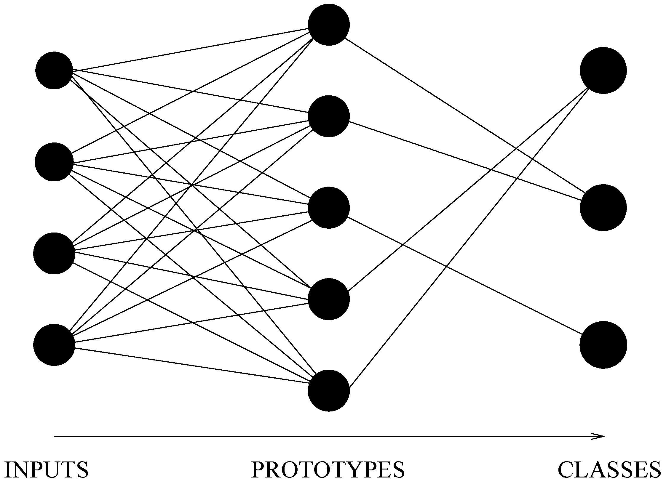
In a previous work [10], the incremental neural network (further called INN) used is a three-layer feedforward neural network that uses prototypes (or exemplars) to perform classification tasks (see Figure 1). Traditional artificial neural networks learn weights for every feature in the input. INNs use a set of representative examples (the prototypes) to model each class. The prototypes are stored in the network’s memory—the networks’s weights—and used to classify new inputs by measuring the similarity between an input and each prototype.

The use of a neural network as support to a prototype-based classifier draws its inspiration from both Grossberg’s and Kohonen’s work. The motivation behind the attempt is to provide a frugal technique to classify labeled data, while providing an explainable approach. Indeed, unlike most neural methods that could be referred to as “deep”, the INN has some features that facilitate its use in an interdisciplinary context.

1.4. Affective Computing

Affective computing is the computing that relates to, arises from, or influences emotion [12]. Visual and auditive modalities are often preferred to physiological data (temperature, heart rate, skin conductance, etc.), because they can be acquired in a non-invasive manner and because they do not require expensive or specific sensors. The field highlights new perspectives to assist people who suffer from affective troubles. According to the World Health Organization [13], in 2019, major depressive disorder (MDD) affects more than 280 million people, including children and adolescents. People suffering from depression often experience sadness, loss of interest, or feelings of guilt for a duration of at least two weeks. Clinically, it is possible to assess the depressive state of an individual using specific tools, such as the Beck Depression Inventory II assessment (BDI-II). The latter consists in a set of 21 questions that result in a score ranging from 0 to 63. For a score inferior to 13, the depression is assessed as minimal; from 14 to 19, as mild; from 20 to 28, as moderate; and as severe above 29.

The challenge series AVEC is aimed at the comparison of multimedia processing and machine learning methods for the automatic recognition of emotion and depression. In its edition of 2014, the organizers provided a dataset composed of video sequences of a subject in front of a recording webcam. In each video, a subject, either male or female, is answering a question about their childhood (freeform database) or reading an excerpt from a book (northwind database). The main purpose behind each database was to compare a situation where people would naturally experience strong feelings to a situation where behaviors could be compared given the same configuration. Each video is annotated with a BDI-II score, allowing for depression classification. A full description of the data can be found in [14], as well as the procedure to download the videos.

1.5. Organization

The rest of the paper is organized as follows. In Section 2, we provide an overview of the uses of prototype-based methods in the literature and provide algorithmic details of the implemented framework. In Section 3, we present some results achieved using the framework, which indicate that it produces promising outcomes on two datasets. These results are discussed in Section 4, and some openings and future research directions are proposed in Section 5.

2. Materials and Methods

In this section, we realize a brief overview of the origins and uses of incremental neural networks and provide in-depth indications on the implementation of the framework.

2.1. Overview

INNs comprise both supervised and unsupervised classification methods, are known to be well-suited to learning from small datasets, and provide explainable models [15].

The use of a neural network as support to a prototype-based classifier draws its inspiration from Kohonen’s self-organizing maps [16]. In a prototype-based neural classifier (further called incremental neural network, or INN), a prototype can be seen as the collection of the weights of a hidden neuron, which can compute a similarity between the stored prototype and a data point. The prototypes and data exist in the same space (through their weight vector), making them understandable, especially for interdisciplinary use-cases and research. Regarding unsupervised learning methods, recent techniques allow us to obtain interesting results from small datasets [17]. The integration of human expertise at an early stage of the training process favors effective analysis and interpretation [18].

The INN is also inspired from Grossberg’s ART model [6] and is based upon key cognitive science concepts. It was initially proposed by Azcarraga and Giacometti [19] and later adapted to supervised classification tasks by Puzenat [20]. More recently, the INN was successfully used in affective computing in order to classify depressive states with respect to the Beck Depression Inventory measurement scale [21]. In this paper, we extend and publish the framework that was used. We also provide algorithmic details and experiments in order to assess the framework.

2.2. Relevant Work

According to [15], prototype-based machine learning methods (PBs) have proven to be effective in various applications. Recent years have seen a growing number of attempts at the development of approaches combining complex models, such as deep neural networks and prototype-based models.

In [22], the authors propose an in-depth review of prototype-based methods. While acknowledging that these methods are not cutting-edge and may not provide outperforming numerical results, they show that they rely on shared mathematical foundations with neural networks and encourage the alliance of PBs with complex models in order to reach explainability over the methods.

In one attempt, the authors of [23] have developed a prototype-based method and network architecture for deep learning (DMR) in order to address a class-imbalanced classification problem. Their solution outperformed others on the hard Caltech-256 benchmark. The core novelty of their approach is in the use of a prototype layer, which they hold responsible for providing an explainable-by-design model. Each new sample is assigned to its nearest prototype. However, in their learning algorithm, they do not make use of a second-nearest prototype, which could probably have given a lever to increase the number of prototypes (which was desired in their use-case).

Eventually, prototype-based networks have successfully addressed a few-shot classification problem, i.e., a task where a classifier has to accommodate new classes not seen in training, given only a few examples of each of these classes [24]. With the help of the prototype-based approach, they used a distance metric in the embedding space to classify new data points. The approach was efficient, as their proposal outperformed previous state-of-the-art few-shot learning methods on several benchmark datasets, including Omniglot and miniImageNet.

2.3. Learning and Control

2.3.1. Learning Algorithm

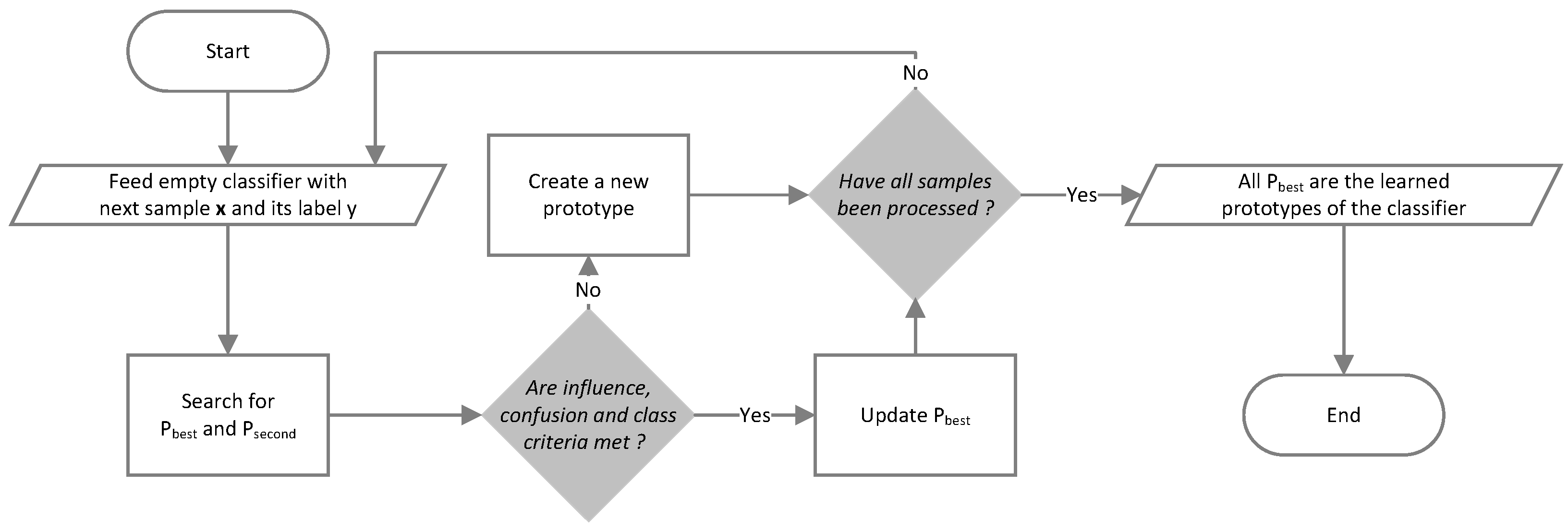
Let $S=\{({\mathbf{x}}_1,y_1),\dots ,({\mathbf{x}}_n,y_n)\}$ be a dataset with $\mathbf{x}\in {\mathbb{R}}^m$ and $y\in \{k_1,\dots ,k_c\}$ a class label. Samples are successively presented to the INN with their class label. Each time the algorithm meets a new class, it creates a new prototype with the first sample that was met with the class. For each $\mathbf{x}$, the algorithm searches the closest prototype $P_{best}$ with respect to a similarity measure $\delta$. If $Class\left(\mathbf{x}\right)\ne Class\left(P_{best}\right)$, a new prototype is created. Otherwise, two conditions are checked:

• $\delta (P_{best},\mathbf{x})\le s_{inf}$, with $s_{inf}\in {\mathbb{R}}^{+}$ the influence threshold. In this case, the sample is said to be under the influence of its best prototype.
• $\delta (P_{best},\mathbf{x})-\delta (P_{second},\mathbf{x})>s_{conf}$, with $s_{conf}\in {\mathbb{R}}^{+}$ the confusion threshold and $P_{second}$ the second-best prototype of $\mathbf{x}$ such as $Class\left(P_{second}\right)\ne Class\left(P_{best}\right)$. In this case, it is said that there is no confusion.

In one of the conditions is not met, then a new prototype is created. Otherwise, the weights of the best prototype are updated to bring it closer to the passing sample. The described algorithm is a winner-takes-all algorithm, as only the winning prototype is activated and updated. Alternatives exist where prototypes in the surroundings of the winning prototype are also updated. A flowchart of the learning algorithm is proposed in Figure 2.

Algorithm

The implemented learning algorithm (Algorithm 1) is proposed as follows:

Algorithm 1: Learning algorithm

Feed the classifier with a sample $\mathbf{x}$ and its label y Search for $P_{best}$ so that $\delta (P_{best},\mathbf{x})$ is minimal Search for $P_{second}$ so that $\delta (P_{second},\mathbf{x})$ is minimal and that $Class\left(P_{second}\right)\ne Class\left(P_{best}\right)$ If: $$\left\{\begin{array}{c}\delta (P_{best},\mathbf{x})\le s_{inf}\hfill \\ \delta (P_{best},\mathbf{x})-\delta (P_{second},\mathbf{x})>s_{conf}\hfill \\ Class\left(P_{best}\right)=Class\left(\mathbf{x}\right)\hfill \end{array}\right.$$ Then update $P_{best}$: $$\forall i\in \{1,\dots ,m\},w_i\leftarrow w_i+\alpha *(x_i-w_i),\mathrm{with}{P}_{best}=\{w_1,\dots ,w_m\}\mathrm{and}\mathbf{x}=\{x_1,\dots$$ $,x_m\}$ Else create a new prototype:       $\forall i\in \{1,\dots ,m\},w_1^{\prime }\leftarrow x_i$ with $P=\{w_1^{\prime },\dots ,w_m^{\prime }\}$       $Class\left(P\right)\leftarrow Class\left(\mathbf{x}\right)$

Each time the algorithm encounters a new class, it creates a new prototype with the first sample presented for this class. Once all the patterns have been presented, the model is composed of all the prototypes learned by the algorithm and can be either used in generalization or relearned (by presenting it with other patterns).

The INN has three control hyperparameters: the influence threshold $s_{inf}$, the confusion threshold $s_{conf}$, and the update coefficient $\alpha$, which controls how close $P_{best}$ will be brought to the passing $\mathbf{x}$. These control hyperparameters address the stability–plasticity dilemma, i.e., considering new samples while not forgetting old ones.

2.3.2. Control

Influence Threshold

The influence threshold $s_{inf}$ of the classifier is the maximal allowed distance $\delta$ between a sample $\mathbf{x}$ and its best prototype $P_{best}$, so that $\mathbf{x}$ is said to be under the influence of $P_{best}$. If a sample does not pass this requirement during the learning phase, then a new prototype is created.

$$\delta (P_{best},\mathbf{x})\le s_{inf}$$

(2)

Confusion Threshold

The confusion threshold $s_{conf}$ helps to discriminate ties at the frontier between distinct classes. It represents a distance between two other distances; the first one being the distance between an observation $\mathbf{x}$ and its best prototype $P_{best}$, and the second being the distance between the very same observation $\mathbf{x}$ and its second-best prototype with a different class $P_{second}$. If this condition is not satisfied, a new prototype is created.

$$\delta (P_{best},\mathbf{x})-\delta (P_{second},\mathbf{x})>s_{conf}$$

(3)

The optimal values for the influence and confusion thresholds strongly rely on the data. Thus, data normalization and variance computation can facilitate optimization.

Update Coefficient

The update coefficient $\alpha \in \left[0,1\right]$ is used when a sample $\mathbf{x}$ passes both requirements of Equations (2) and (3), i.e., when $\mathbf{x}$ is under the influence of its best prototype and when there is no risk of confusion. In this case, the weights of $P_{best}$ are updated to bring it closer to the passing sample. Let w be the weight of $P_{best}$. Then the update can be expressed as:

$$\forall i\in \{1,\dots ,m\},w_i\leftarrow w_i+\alpha \ast (x_i-w_i)$$

(4)

A large value for $\alpha$ implies that the prototypes will be strongly brought closer to passing samples, thus increasing the overall prototype cardinality. In contrast, a low value limits the prototypes’ moving, thus limiting their cardinality.

Similarity Measures

Computing the similarity between the prototypes and samples is performed with a similarity measure or with a distance, commonly chosen with respect to the problem to solve. This possibility makes INNs flexible and adaptable. Among the common measures, we have the Minkowski family measures (see Equation (5)), where $p=2$ is like computing an Euclidean distance.

$$d_{mink}(x,y)={\left(\sum _{i=1}^n{\left|x_i-y_i\right|}^p\right)}^{1/p}$$

(5)

Prototype Ratio

During the learning phase, an interesting metric to monitor is the ratio of prototypes $\rho$, which is the number of stored prototypes divided by the size of the learning set. Low $\rho$ values are preferable, as they show that the classifier could learn effectively from the data, implying that the hyperparameters are correct. In contrast, high values are a sign of overfitting. Thus, learning can be stopped whenever $\rho$ is above a defined threshold.

2.4. Generalization and Interpretation

2.4.1. Generalization Algorithm

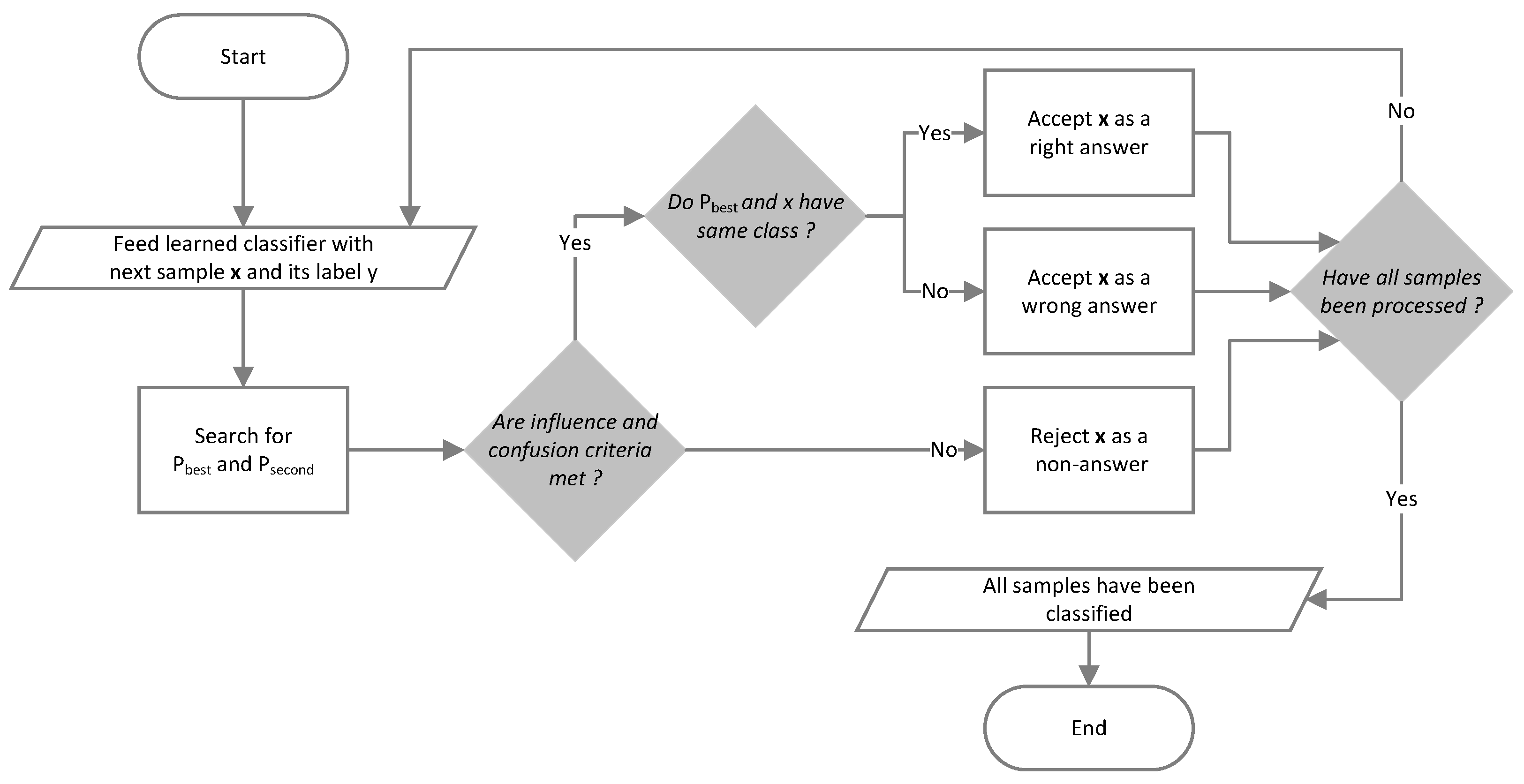
Generalization follows the same rules as training, but prototypes are no longer created or modified during this step. For each new pattern $\mathbf{x}$, see Algorithm 2:

Algorithm 2: Generalization algorithm

Feed the classifier with a sample $\mathbf{x}$ Search for $P_{best}$ so that $\delta (P_{best},\mathbf{x})$ is minimal Search for $P_{second}$ so that $\delta (P_{second},\mathbf{x})$ is minimal and $Class\left(P_{second}\right)\ne Class\left(P_{best}\right)$ If$P_{best}$ is too far from $\mathbf{x}$ or if there is a risk of confusion: $$\left\{\begin{array}{c}\delta (P_{best},\mathbf{x})>s_{inf}\hfill \\ \mathrm{or}\hfill \\ \delta (P_{best},\mathbf{x})-\delta (P_{second},\mathbf{x})\le s_{conf}\hfill \end{array}\right.$$ Then reject $\mathbf{x}$ (“non-answer”) Else if class of $P_{best}$ is that of $\mathbf{x}$,        Then $\mathbf{x}$ is recognized (“right answer”)        Else $\mathbf{x}$ is not recognized (“wrong answer”)

At this step, computation of the distances between the prototypes and examples is very power-consuming and takes $O\left(\right|P\left|\right)$ operations. In order to increase the generalization speed, the prototypes are organized in a $kd$-tree for faster distance comparison. Note that it is not relevant to use $kd$-trees during learning, as the prototypes are constantly updated. Computation of the $kd$-trees at each update would take more time than a classical distance computation. A flowchart for the generalization algorithm is proposed in Figure 3.

2.4.2. Answers

The INN can provide three kinds of answers. Right answers are provided when all conditions are met and when the label of the test sample is the same as that of the best prototype. Intuitively, the higher the number of correct answers, the better the quality of the classification. Wrong answers are provided when a condition was not met, but the label of the test was still matching that of the best prototype.

Non-answers are provided in any other situation, i.e., when the best prototype is too far from the sample or when the risk of confusion is too high. A non-answer is comparable to a human judgment when confronted with an unknown situation, when they would answer I don’t know. This answer marks the absence of a decision rather than a correct or incorrect decision. The number of non-answers can be considered a reliability indicator for the system. Thus, a high number of non-answers would mean that the system is likely not reliable, while right answers, in turn, would be more reliable.

2.5. Implementation Details

The classifier has been implemented from scratch by implementing the conceptualized algorithms found in the literature about prototype-based incremental neural networks [6,19,20]. The algorithm is implemented in Python 3.x and uses scientific libraries such as Numpy [25] and MatplotLib [26]. We chose the HDF5 scientific data format [27] as an alternative to Pandas, as it could handle larger volumes and allowed more efficient read and write operations. However, the framework can still be fed with CSV files. Later, we adapted our source code so that it complies with the Scikit-Learn API [28], mainly for the fit, score, and predict operations. Sklearn [29] is also used to compute metrics and distances.

In its development phase, the framework was used and tested on several toy datasets, including (but not limited to) iris, wine, breast cancer, and MNIST. However, it was designed with the goal of being applied in the field of affective computing, mainly on multimodal data for the emotion and depression classification tasks [10,11,21]. Thus, some utilities were left in the published source code to address these tasks, although they do not alter the genericity of the algorithm. Listing 1 proposes a minimal working example to start using the implemented framework.

The code source of the framework is available as a supplementary material linked at the end of this paper.

Listing 1. Minimal working example for the implemented INN framework.

3. Results

In this section, we provide two results that aim to show that the implemented INN can provide state-of-the-art results on a toy dataset, as well as interesting results on more complex video data.

3.1. Studying Frugality of INN

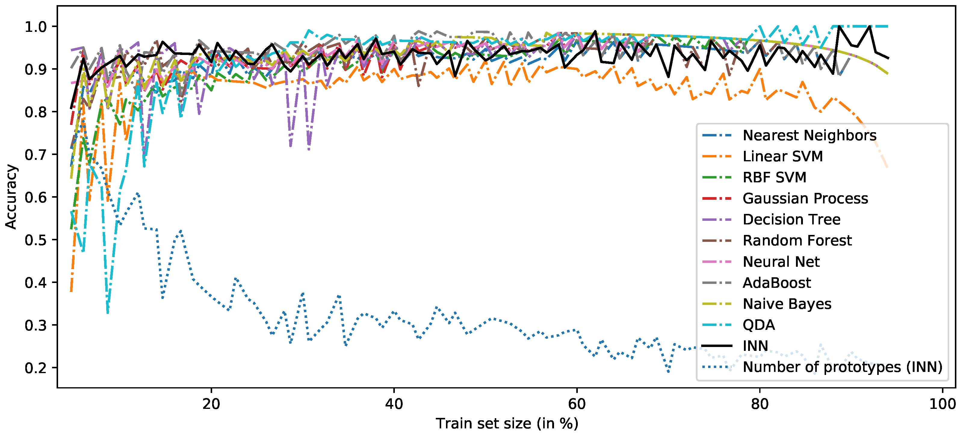
As stated earlier, frugality refers to the ability of a classifier to learn effectively from a relatively low number of observations, while achieving state-of-the-art accuracy performance. For this experiment, we use the classic iris dataset in order to guarantee reproductibility and ensure baseline comparison. The iris dataset contains measurements of four features of three different species of iris flowers: sepal length, sepal width, petal length, and petal width. The dataset is balanced and consists of 150 samples of three classes (setosa, versicolor, and virginica). To study the frugality of the INN, we split the dataset into a training set and a validation set in a stratified hold-out fashion. The size of the training set varies from 5% to 95% of the total dataset, and the remaining data are used for validation. We repeat this process for each split, and for each split, we train several classifiers on the training set and test them on the validation set. The classifiers include the INN and other common classifiers, such as nearest neighbors, linear SVM, and random forests.

In order to study the frugality of the INN, it is interesting to determine how many training samples the classifier requires to achieve state-of-the art performance on the dataset. A a toy dataset, a baseline accuracy for iris can be set to 0.85, noting that this baseline does not take into account the split size.

Figure 4 shows the compared plot of accuracies for the varying split sizes. From the compared accuracies computed, it appears that the INN outperforms the baseline from the split 6/94 (i.e., 6% of examples for training and the remaining 94% for validation). However, the high ratio of prototypes indicates that the classifier likely overfitted for splits before 15/75, as $\rho$ is above 0.4. As the accuracy increases with the training set size to stabilize over 0.9, the ratio of prototypes progressively drops to less than 30%. The hyperparameters of the INN were found using a grid-search approach and were set to $s_{inf}=1$, $s_{conf}=0.1$, and $\alpha =0.1$. The parameters of the other classifiers were taken from the literature and are detailed in the source code.

3.2. Application to Affective Computing

The INN implementation was initially designed to address multimodal classification problems in affective computing, and more specifically concerning emotion and depression classification. Several results have been published [11,21], including a live prototype demonstration [30].

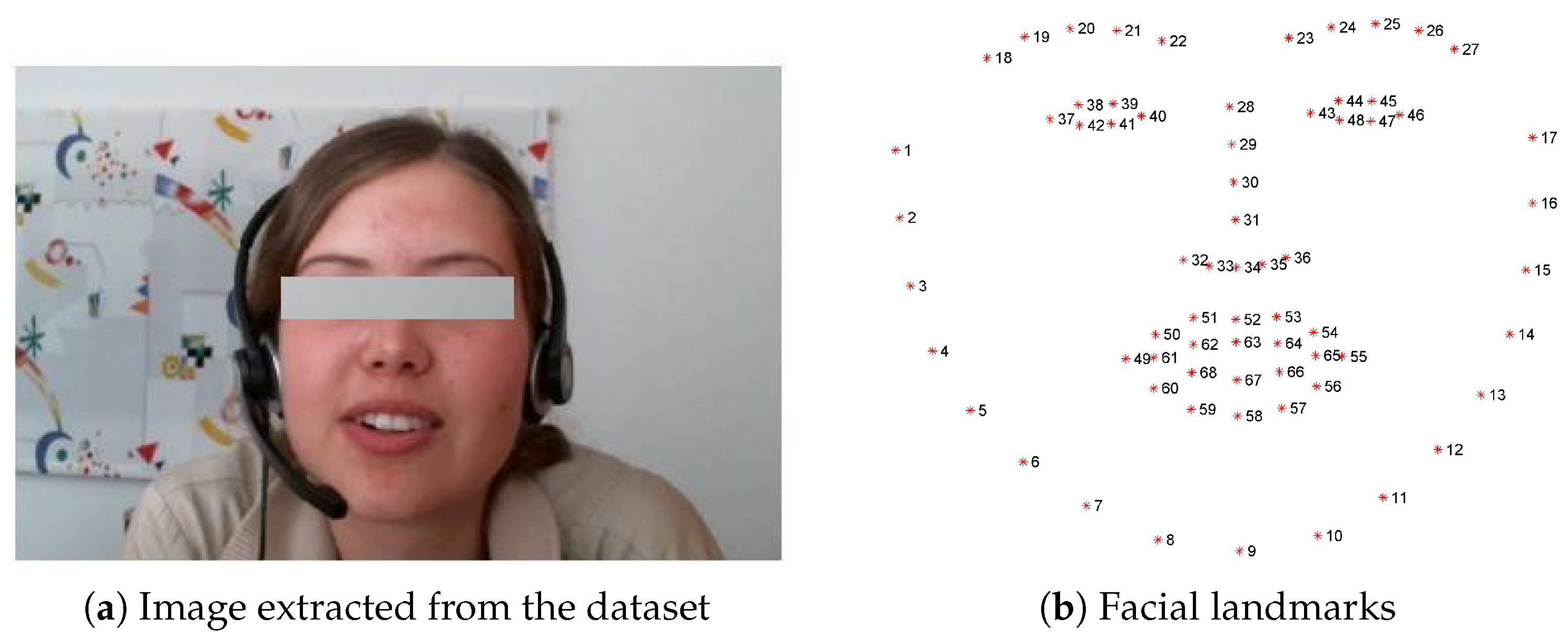
This experiment was previously published in [10], and consists of the use of the INN to predict the depressive score of subjects in the dataset of the AVEC2014 challenge. The dataset consists of 150 task-oriented videos of human–computer interaction scenarios. In each video, there is only one subject (see Figure 5), and the whole dataset contains 84 subjects. The recordings range from 20 to 50 min, totaling 240 h. The subjects’ mean age was 31.5 years (SD = 12.3, range 18–63), and the recordings took place in quiet settings. The videos are labelled with a BDI-II score ranging from 0 to 63. Detailed information about the dataset can be found in [14]. In particular, it is worth noting that the classes are not ideally balanced in data, with only a few to no videos for higher depressive scores. The descriptors used were designed to estimate the quantity of movement on the face (micro-movements) and of the face itself (head gesture). For a given video, a set of 68 facial two-dimensional landmarks is extracted from each image (see Figure 5. The faces are aligned and their sizes are standardized by rotating the shapes by an angle $\theta$ with a scale factor S. This similarity transform can be represented by the matrix in Equation (6) and was estimated using OpenCV [31].

$$M=\left[\begin{array}{cc}{s}_{x}cos\left(\theta \right)& sin\left(\theta \right)\\ -sin\left(\theta \right)& s_{y}cos\left(\theta \right)\end{array}\right]$$

(6)

The final descriptor is composed of a rolling standard deviation $\sigma$ of facial points of interest over an overlapping window of time of size ${\mathsf{T}}_{\mathsf{win}}$ with step ${\mathsf{T}}_{\mathsf{step}}$. The resulting features are aimed at capturing slow- and long-changing patterns occurring in the data, as well as their dynamics. This manner of processing data is not novel and was applied by [14], still in the context of affective computing. Let $x_{jt}$ be the jth component of an observation at time t. Then, the resulting descriptor component $x_{jt}^{\prime }$ can be expressed as in Equation (7).

$$\begin{array}{cc}\hfill x_{jt}^{\prime }& =\sigma \left(x_{jt},x_{j(t+1)},\dots ,x_{j(t+{\mathsf{T}}_{\mathsf{win}})}\right)\hfill \\ \hfill x_{j(t+1)}^{\prime }& =\sigma \left(x_{j(t+{\mathsf{T}}_{\mathsf{step}})},x_{j(t+{\mathsf{T}}_{\mathsf{step}}+1)},\dots ,x_{j(t+{\mathsf{T}}_{\mathsf{step}}+{\mathsf{T}}_{\mathsf{win}})}\right)\hfill \end{array}$$

(7)

An INN has been trained with a leave-one-subject-out cross-validation strategy. For each round of validation, one subject is left out from the training set and used as the validation set. This process is repeated for all subjects in the dataset, and the results are averaged to obtain an estimate of the model’s performance. This strategy ensures that the model does not learn to associate a specific subject with a depressive state, which could bias the results. The classification errors of the cross-validation are provided in

Table 1. Results for the leave-one-out cross-validation of the classification of BDI-II scores on the AVEC2014 corpus.

	Freeform	Northwind
RMSE	10.31	10.75
MAE	9.81	10.39
$\rho$	0.26	0.34

. As the depressive scores range from 0 to 63, an error around 10 could be regarded as “fair” given the complexity of the data, the validation strategy, and the nature of the classifier.

It is also worth noting that the classifier struggled more with severe depressive states, while achieving smaller errors for other states. For instance, on the freeform dataset, the RMSE for minimal depressive states (scores ranging from 0 to 13) is as low as 8.31 (10.31 overall) versus 20.80 for severe depressive states (scores close to 63). This can be explained by the balancing of data, which features more instances of minimal to moderate depressive states.

4. Discussion

Our first experiment was intended to compare the frugality of the INN to common classifiers using a state-of-the-art dataset. The results show that the INN could learn effectively from a limited volume of data, while outperforming most classifiers. In the literature, INNs have proved to be able to achieve interesting performances, even on much more complex data. Although the success in achieving a high prediction accuracy on the iris dataset is not an advance, it remains an obligatory step for any new framework that claims to work. However, these results have to be put in a broader context, especially at the time where cutting-edge algorithms are available and outperform so-called common traditional techniques.

A distinguishing point inherent to INNs is their ability to add new observations to the model without the need of starting the learning phase over, fully enabling its incremental power. Moreover, such techniques are appreciated in interdisciplinary research (such as in cognitive science, psychiatry, affective computing, etc.), where explaining the model is crucial. As a prototype stands in the same space as the data, is becomes possible to observe and interpret any prototype just like any input sample.

Our second experiment was led on an affective database and intended to predict the depressive score of subjects in terms of BDI-II score. The INN achieved an RMSE/MAE of 10.31/9.81 on the freeform database, which is better than the RMSE/MAE of 10.31/9.81 obtained on northwind. This difference could be explained by the fact that subjects are more inclined to express feelings while relating a memory than while reading an excerpt (see the description of each database in Section 1.4). It is worth noting that the experiment was conducted during a study in which the process had to be explained to care professionals. Further interpretations could allow us to understand which face micro-movements could unveil depressive states [10].

5. Conclusions

The main contribution of this research is the implementation of a prototype-based neural network that can be reused for a wide variety of applications. To the best of our knowledge, there is no such existing public implementation. This novelty could be quite interesting for the community, as prototype-based algorithms are frugal, versatile, and interpretable. Future research directions include the improvement of the INN and its embedding in a bidirectional associative memory.

References

- Abiodun, O.I.; Jantan, A.; Omolara, A.E.; Dada, K.V.; Umar, A.M.; Linus, O.U.; Arshad, H.; Kazaure, A.A.; Gana, U.; Kiru, M.U. Comprehensive review of artificial neural network applications to pattern recognition. IEEE Access 2019, 7, 158820–158846. [Google Scholar] [CrossRef]
- Manohar, B.; Das, R. Artificial Neural Networks for the Prediction of Monkeypox Outbreak. Trop. Med. Infect. Dis. 2022, 7, 424. [Google Scholar] [CrossRef] [PubMed]
- Wang, Y.; Song, W.; Tao, W.; Liotta, A.; Yang, D.; Li, X.; Gao, S.; Sun, Y.; Ge, W.; Zhang, W.; et al. A systematic review on affective computing: Emotion models, databases, and recent advances. Inf. Fus. 2022, 83–84, 19–52. [Google Scholar] [CrossRef]
- Sujyothi, A.; Acharya, S. Dynamic Malware Analysis and Detection in Virtual Environment. Int. J. Mod. Educ. Comput. Sci. 2017, 9, 48–55. [Google Scholar] [CrossRef]
- Wang, J.; Yang, S.; Jia, J. Prototype Selection with Applications to Multimodal Emotion Recognition from Speech and Text. IEEE Trans. Affect. Comput. 2020, 3, 350–357. [Google Scholar]
- Grossberg, S. Nonlinear neural networks: Principles, mechanisms, and architectures. Neural Netw. 1988, 1, 17–61. [Google Scholar] [CrossRef]
- Kohonen, T.; Kohonen, T. Learning vector quantization. In Self-Organizing Maps; Springer: Berlin/Heidelberg, Germany, 1995; pp. 175–189. [Google Scholar]
- Hussaindeen, A.; Iqbal, S.; Ambegoda, T.D. Multi-label prototype-based interpretable machine learning for melanoma detection. Int. J. Adv. Signal Image Sci. 2022, 8, 40–53. [Google Scholar] [CrossRef]
- Fazel Zarand, M.; Teimouri, M.; Zaretalab, A.; Hajipour, V. A prototype-based classification using extended imperialist competitive algorithm. Sci. Iran. 2017, 24, 2062–2081. [Google Scholar] [CrossRef]
- Cholet, S. Evaluation Automatique des éTats éMotionnels et déPressifs: Vers un Outil de Prévention des Risques Psychosociaux. Ph.D. Thesis, Université des Antilles, Pointe-a-Pitre, France, 2019. [Google Scholar]
- Cholet, S.; Paugam-Moisy, H.; Régis, S. Bidirectional Associative Memory for Multimodal Fusion: A Depression Evaluation Case Study. In Proceedings of the 2019 International Joint Conference on Neural Networks (IJCNN), Budapest, Hungary, 14–19 July 2019; pp. 1–6. [Google Scholar]
- Picard, R.W. Affective Computing; MIT Press: Cambridge, MA, USA, 1997. [Google Scholar]
- World Health Organization. Mental Disorders. 2023. Available online: https://www.who.int/news-room/fact-sheets/detail/mental-disorders (accessed on 17 March 2023).
- Valstar, M.; Schuller, B.; Smith, K.; Almaev, T.; Eyben, F.; Krajewski, J.; Cowie, R.; Pantic, M. AVEC 2014: 3D Dimensional Affect and Depression Recognition Challenge. In Proceedings of the 4th International Workshop on Audio/Visual Emotion Challenge, Orlando, FL, USA, 7 November 2014; Association for Computing Machinery: New York, NY, USA, 2014; pp. 3–10. [Google Scholar] [CrossRef]
- Biehl, M.; Hammer, B.; Villmann, T. Prototype-based models in machine learning. WIREs Cogn. Sci. 2016, 7, 92–111. [Google Scholar] [CrossRef] [PubMed]
- Kohonen, T. Self-Organizing Maps, 3rd ed.; Springer Series in information Sciences; Springer: Berlin, Germany, 2001. [Google Scholar]
- Biabiany, E.; Bernard, D.C.; Page, V.; Paugam-Moisy, H. Design of an expert distance metric for climate clustering: The case of rainfall in the Lesser Antilles. Comput. Geosci. 2020, 145, 104612. [Google Scholar] [CrossRef]
- Bernard, D.; Biabiany, E.; Cécé, R.; Chery, R.; Sekkat, N. Clustering analysis of the Sargassum transport process: Application to beaching prediction in the Lesser Antilles. Ocean Sci. 2022, 18, 915–935. [Google Scholar] [CrossRef]
- Azcarraga, A.; Giacometti, A. A prototype-based incremental network model for classification tasks. In Proceedings of the Fourth International Conference on Neural Networks and their Applications, Nimes, France, 4 November 1991. [Google Scholar]
- Puzenat, D. Parallélisme et Modularité des Modèles Connexionnistes. Ph.D. Thesis, École Normale Supérieure (Sciences), Lyon, France, 1997. [Google Scholar]
- Cholet, S.; Paugam-Moisy, H. Prototype-based Classifier for Automatic Diagnosis of Depressive Mood. In Proceedings of the 2018 International Conference on Biomedical Engineering and Applications (ICBEA), Funchal, Portugal, 9–12 July 2018; pp. 1–6. [Google Scholar] [CrossRef]
- Saralajew, S.; Holdijk, L.; Rees, M.; Villmann, T. Prototype-based neural network layers: Incorporating vector quantization. arXiv 2018, arXiv:1812.01214. [Google Scholar]
- Angelov, P.; Soares, E. Towards deep machine reasoning: A prototype-based deep neural network with decision tree inference. In Proceedings of the 2020 IEEE International Conference on Systems, Man, and Cybernetics (SMC), Toronto, ON, Canada, 11–14 October 2020; pp. 2092–2099. [Google Scholar]
- Snell, J.; Swersky, K.; Zemel, R. Prototypical networks for few-shot learning. In Proceedings of the 31st International Conference on Neural Information Processing Systems, Long Beach, CA, USA, 4–9 December 2017; Volume 30. [Google Scholar]
- Harris, C.R.; Millman, K.J.; van der Walt, S.J.; Gommers, R.; Virtanen, P.; Cournapeau, D.; Wieser, E.; Taylor, J.; Berg, S.; Smith, N.J.; et al. Array programming with NumPy. Nature 2020, 585, 357–362. [Google Scholar] [CrossRef] [PubMed]
- Hunter, J.D. Matplotlib: A 2D graphics environment. Comput. Sci. Eng. 2007, 9, 90–95. [Google Scholar] [CrossRef]
- The HDF Group. Hierarchical Data Format, Version 5. 1997–2023. Available online: https://www.hdfgroup.org/HDF5/ (accessed on 17 March 2023).
- Buitinck, L.; Louppe, G.; Blondel, M.; Pedregosa, F.; Mueller, A.; Grisel, O.; Niculae, V.; Prettenhofer, P.; Gramfort, A.; Grobler, J.; et al. API design for machine learning software: Experiences from the scikit-learn project. In Proceedings of the ECML PKDD Workshop: Languages for Data Mining and Machine Learning, Prague, Czech Republic, 23–27 September 2013; pp. 108–122. [Google Scholar]
- Pedregosa, F.; Varoquaux, G.; Gramfort, A.; Michel, V.; Thirion, B.; Grisel, O.; Blondel, M.; Prettenhofer, P.; Weiss, R.; Dubourg, V.; et al. Scikit-learn: Machine Learning in Python. J. Mach. Learn. Res. 2011, 12, 2825–2830. [Google Scholar]
- Cholet, S.; Paugam-Moisy, H. Vers un outil pour la prévention des risques psychosociaux. In Proceedings of the Workshop sur les Affects, Compagnons Artificiels et Interactions, Ile d’Oleron, France, 3–5 June 2020. hal-02933490. [Google Scholar]
- Bradski, G. The OpenCV Library. Dr. Dobbs J. Softw. Tools 2000, 25, 120–125. [Google Scholar] [CrossRef]