An Automatic Tomato Growth Analysis System Using YOLO Transfer Learning

Abstract

In recent years, Japan’s agricultural industry has faced a number of challenges, including a decline in production due to a decrease in farmland area, a shortage of labor due to a decrease in the number of producers, and an aging population. Therefore, in recent years, smart agriculture using robots and IoT has been studied. A caliper is often used to analyze the growth of tomatoes in a plant factory, but this method may damage the stems and is also hard on the measurer. We developed a system that detects them through image analysis and measures the thickness of stems and the length between flower clusters and growing points. The camera device developed in this study costs about USD 150 and once installed, it does not need to be moved unless it malfunctions. The camera device reduces the effort required to analyze crop growth by about 80%.

1. Introduction

In recent years, Japan’s agricultural industry has faced a number of challenges, including a decline in production due to a decrease in farmland area, a shortage of labor due to a decrease in the number of producers, and an aging population [1]. In 2015, 64.9% of agricultural workers were aged 65 years old or above; however, by 2020, this percentage had increased to 69.8%. In addition, the arable land area in Japan has been decreasing, as shown in Figure 1. The total area of arable land as of July 2020 was approximately 4.37 million hectares. Therefore, in recent years, smart agriculture using robots and IoT has been studied. Smart agriculture aims to solve the shortage of human labor by automating tasks that are normally performed by humans. It also aims to improve the efficiency of work by using computers to manage and analyze data on crops and the environment, thereby increasing production per unit area and improving quality.

The purpose of this research was to automatically analyze the growth status of tomatoes using camera images. To achieve that, farmers measured the thickness of the stems near the flower clusters, and the length of flower clusters and growing points. In fact, a caliper is often used to analyze the growth of tomatoes in a plant factory, but this method may damage the stems and also put strain on the person conducting the measurement [2]. We believe that this required time can be reduced by using cameras installed on farms and image analysis techniques. In this study, we aimed to create a system to perform such analysis. This system should be inexpensive and easy to use so that farmers who are not familiar with computers can easily adopt it. Therefore, our goal is to obtain sufficient measurement data with a small number of cameras by using cameras with a pan-tilt function that can capture multiple plants. Additionally, another objective of this work is to reduce the cost of the hardware used in this system as much as possible, and to create a system that is easy to use and does not require complicated operations by the user.

2. Related Work

Previously, Suma presented the challenges of integrating farmers’ experience and knowledge with state-of-the-art technology in traditional agriculture and proposed a model that utilizes cameras and various sensors to detect features of the farm environment to solve these challenges [3].

Deep neural networks have also been used for plant cultivation. In 1999, Zaidi et al. used a small neural network to detect plant growth [4]. In their experiments, the number of units of the network was only seven in the input layer, eight in the hidden layer, and five in the output layer.

Nagano et al. employed a plant growth detection method based on leaf movements [5]. In their study, the changes in the movement of lettuce leaves over time were extracted as features. These features were analyzed using a growth prediction neural network model to predict the growth state.

Huang et al. proposed a region-based convolutional neural network (R-CNN) model for tomato cultivation that uses images to determine whether the fruit is ripe and automatically determines when to harvest in real time [6].

In 2019, Trung-Tin et al. used 571 tomato images to train and provide a CNN model to recognize the nutrient deficiency status of tomatoes [7]. The model was able to predict calcium (Ca), potassium (K), and nitrogen (N) deficiency states with accuracies as high as 91%.

In 2021, Mubashiru Olarewaju Lawal proposed a model called YOLO-Tomato, a modification of YOLOv3 [8]. It allowed tomato detection in complex environments and achieved 99.5% AP in the best model. This was more accurate than the SOTA model at the time.

In 2022, Arunabha et al. proposed a real-time object detection framework Dense-YOLOv4 based on an improved version of the YOLOv4 algorithm introducing DenseNet [9]. In orchards, it is important to detect the growth stage of leaves based on their quantity, size, and color in order to increase the yield. By applying DenseNet-fused YOLOv4, we were able to detect growth stages with high accuracy. This framework can be extended to detect various crops, diseases, etc.

3. System Design

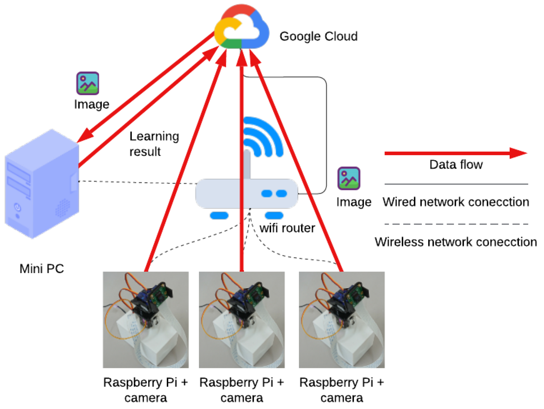
The network architecture and data flow of the system are shown in Figure 2. First, each camera device is placed in the field. It takes an image of the area to be photographed and uploads the image to Google Drive. The PC downloads the images uploaded to Google Drive, performs image analysis, and outputs the measurement data. Finally, the measurement data are uploaded in CSV format to a specific shared folder on Google Drive, and the irrigation system can access the measurement data.

3.1. Camera Device

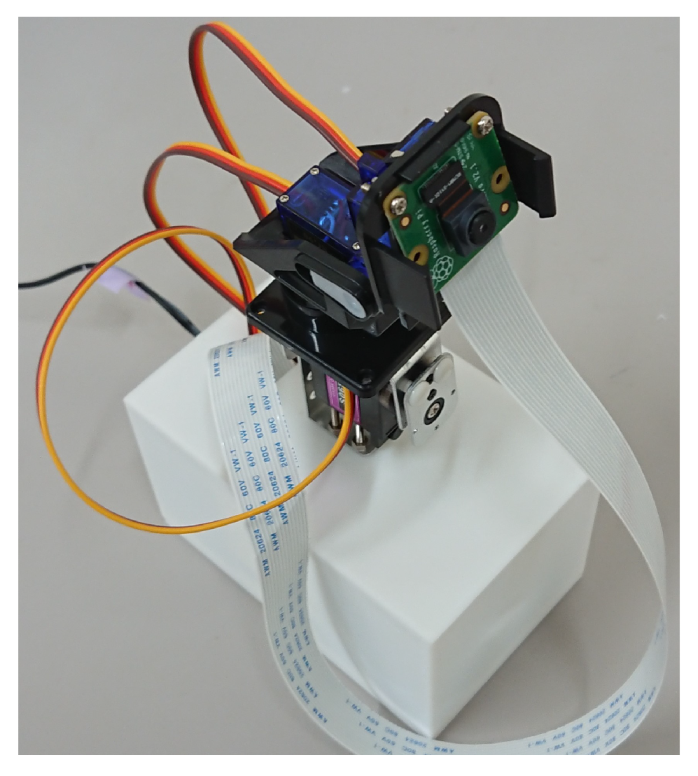
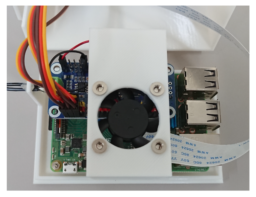
The exterior and interior of the camera device are shown in Figure 3 and Figure 4, respectively. The device is a small camera with a Raspberry Pi, a 3-axis pan-tilt camera mount, and can move the viewpoint. The Raspberry Pi, pulse-width modulation (PWM) servo driver board, and other components are housed in a 3D-printed case, and a 3-axis pan-tilt camera mount is attached to the top of the case. In order to prevent the Raspberry Pi from overheating during field use, it is necessary to use a case with a cooling fan to cover the Raspberry Pi. There were no cases with cooling fans on the market, so we used a 3D printer to make our own case, which consists of two parts: a base to hold the Raspberry Pi and a lid to cover it. The specifications of the camera device used are shown in

Table 1. List of the specifications of the camera [10].

Name	Raspberry Pi Camera V2
Still picture resolution	3280 × 2464
Image sensor	Sony IMX 219 PQ CMOS image sensor in a fixed-focus module.
Lens size	1/4”
Dimensions	23.86 × 25 × 9 mm
Image format	JPEG

.

The servomotor and camera can be controlled using a Raspberry Pi. In addition, images can be uploaded to a shared file environment, such as Google Drive, by connecting to the Internet using a Wi-Fi environment in the field. A 3-axis pan-tilt camera mount using servomotors is created to enable a wide range of imaging with a single camera device. The servomotors are connected to Raspberry Pi via a PWM servo driver equipped with a PCA9685 controller; this controlled multiple servomotors by sending commands to the PWM servo driver via I2C communication to control their angle. For the camera, we used a dedicated camera module for Raspberry Pi. The camera has a resolution of 8 megapixels, which is sufficient for image analysis. In addition, the small size and weight of the board allows it to be moved by a low-torque motor when installed in the camera mount. The camera device can be connected to a network via Wi-Fi or wired cables, and the image data can be sent to a PC for image analysis via Google Drive.

Software Design

The camera device is programmed to run on a Raspberry Pi; specifically, on a Raspberry Pi OS using Python 3.7. The ‘crontab’ command is used to set the program to run at startup. This allows the system to run automatically when Raspberry Pi is turned on. The three functions of this program are: (1) change the viewing direction of the camera by controlling the servomotors, (2) capture images, and (3) upload the captured images to Google Drive. The shooting time to capture images is predetermined by the program, and images are captured at regular intervals during the day. The camera angle is changed slightly at each shooting time to capture images in all possible directions. All captured images are saved in a specific folder on Google Drive. To operate Google Drive using Python, we used the PyDrive module that manipulates the Google Drive application programming interface (API).

3.2. Image Analysis System

In the system shown in Figure 2, an image analysis program runs on a PC. The execution environment is Windows 10 and the language used is Python 3.7. To run this program regularly, we need to set it to run automatically at midnight every day using the Windows task scheduler. The system downloads all images taken by the camera device on the previous day from Google Drive at 00:00 every day, executes the image analysis program, converts the output measurement data into a CSV file, and uploads it to the folder where the measurement data is stored in Google Drive. The steps of the process from downloading the images to uploading the measurement data are described in the list below.

• Download images from Google Drive.
• Correct image distortion.
• Detect stem, target part of stem diameter measurement (target stem), and growing point (seichouten in Japanese) using YOLO.
• Determine the same plant from the label of each detected part.
• Detect circles by Hough transform of reference balls.
• Extract the contour part of the stem by segmentation of the ‘target stem’ part of the image.
• Measure the thickness of the stem in pixels.
• Convert pixels to actual stem diameter length using neighboring reference balls.
• Measure the distance between the ‘target stem’ and the growing point using a reference ball.
• Summarize measurement data and convert them to CSV format.
• Upload the CSV file to Google Drive.

Google Drive file download upload operations use PyDrive as well as a camera device.

3.2.1. Image Distortion Correction

Image distortion correction by camera calibration is done using the OpenCV image processing library. OpenCV includes functions for calculating the parameters required for calibration using a chessboard and for calibrating the image with those parameters. Using the former function, we estimate the parameters from the images taken by the camera module of Raspberry Pi. The system’s program uses these parameters to calibrate all images.

3.2.2. Object Detection with YOLO

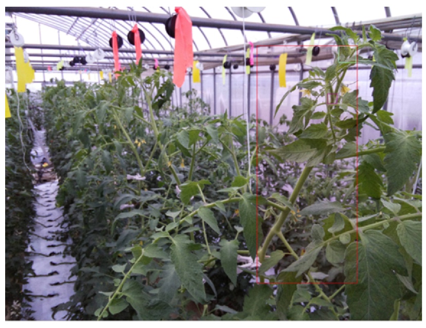
Transfer learning is performed using YOLOv5 to detect tomato plant units. We trained on a pre-trained model using the Coco 2017 dataset (apple detection) [11]. Approximately 1100 images of tomatoes taken in the field were used for training. The object detection targets were stems, ‘target stem’, and growing point, and each part was labeled by surrounding the training image with a rectangle, as shown in

Table 2. Labels and description.

Label	Description
stem	The entire stem including the top of the plant
target stem	The stem connected to the flower
seichouten (growing point)	The point where the plant grows

. The images labeled using these criteria are shown in Figure 5. The training on YOLOv5 was performed with a batch size of 12 and an epoch count of 140 using Mosaic data augmentation and SGD. The trained model used for training was YOLOv5x. Hyperparameters are defaults unless otherwise noted.

YOLO [12] is widely used for real-time object detection such as face recognition and multi-target tracking. Since its release in 2016, YOLO has been updated several times, with the latest version being YOLOv5, which has improved accuracy and performance [13]. The benefits of YOLO are widely applied to the object detection domain, and its performance has been optimized. It is also possible to perform object detection on Raspberry Pi. In addition, YOLO models have been pre-trained on various datasets, allowing for transfer learning of datasets. Hence, YOLO has been optimized for object recognition and highly evaluated for its accuracy and performance. We considered deep learning segmentation of the entire image, but found that generating a dataset for this purpose was challenging and required significant time and resources. Therefore, we decided to use YOLOv5, a bounding box-based object detection method that is easier to create datasets. YOLO has also been used for plant detection [8,9] and is suitable for this system.

3.2.3. Identification of Same Strain from Each Detected Label

The next step is to determine the same strain based on the labels of each detected region. This step alternates between the following two processes: the first one is to determine if the labels are for the same plant from images taken at different times, and the second one is to determine whether the labels ‘stem’, ‘target stem’, and ‘seichouten’ are for the same plant from a single image. These processes are necessary because the labels of multiple strains can be detected in a single image. The first process is to determine the degree of overlap of labels of the same type for each label detected in images taken at different times and at the same shooting angle and to determine whether the labels are of the same plant if they are above a certain threshold value. If the overlap is greater than the threshold value, the labels are considered to be from the same plant. This is based on the fact that the position of labels does not change significantly even if the plant is growing, unless the shooting time to capture images is far apart. In this process, if the attracting string is pulled down, the position of the plant is shifted significantly, and the same plant cannot be tracked. The second process is to determine the overlap between ‘stems’ and ‘target stem’, and between the ‘stem’ and ‘seichouten’ labels; if there is even a small overlap, it is determined to be the same plant. If there are multiple flower clusters in the bloom, multiple ‘target stems’ are detected for a single stem. In this case, the label added above is given priority in the image analysis. In addition, multiple ‘seichouten’ may be detected for a single stem when the side shoots are not processed and extended. However, if the side shoots are not processed for a long time, they often grow higher than the main stem; in this case, accurate measurement is not possible.

3.2.4. Reference Ball Detection

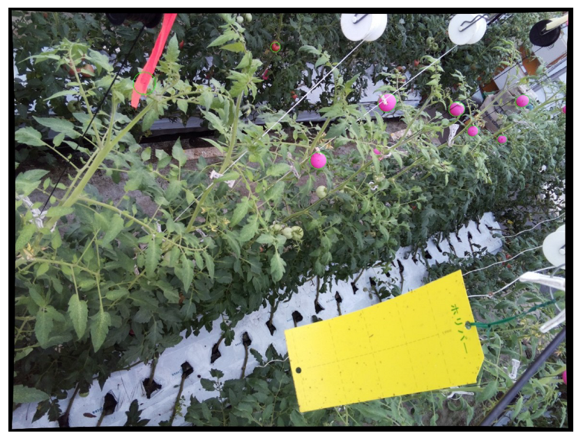
Next, we estimate the diameter of the reference ball in the image by detecting the circle using Hough transform. First, the pink pixels in the image are extracted by setting a threshold value, and a binary image is generated. The image is then smoothed to remove noise and circle detection is performed using the function of OpenCV. The Hough transform can detect circles even if leaves hide a part of the circle. However, false positives are likely to occur. Therefore, to determine whether the detected circle is valid, we checked the number of pink pixels included in the circle and eliminated them if they were below the threshold. OpenCV’s image calibration process can correct the distortion of a flat surface in 3D space, but a sphere such as a ping pong ball will be distorted into an ellipse as it moves away from the center of the image. Therefore, the reference ball may not be accurately detected by circle detection using Hough transform. Therefore, by using contour extraction and ellipse fitting functions of OpenCV, we can detect the elliptical reference sphere. The detected circles and ellipses are circled in green in Figure 6. In this experiment, a pink reference ball was used; nevertheless, red tomatoes and red markers hanging above the field were detected incorrectly.

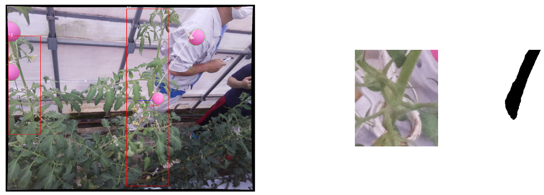
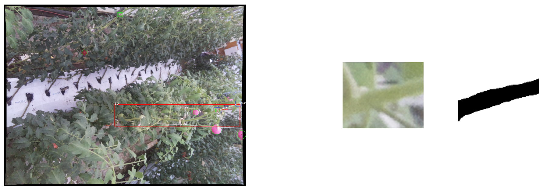
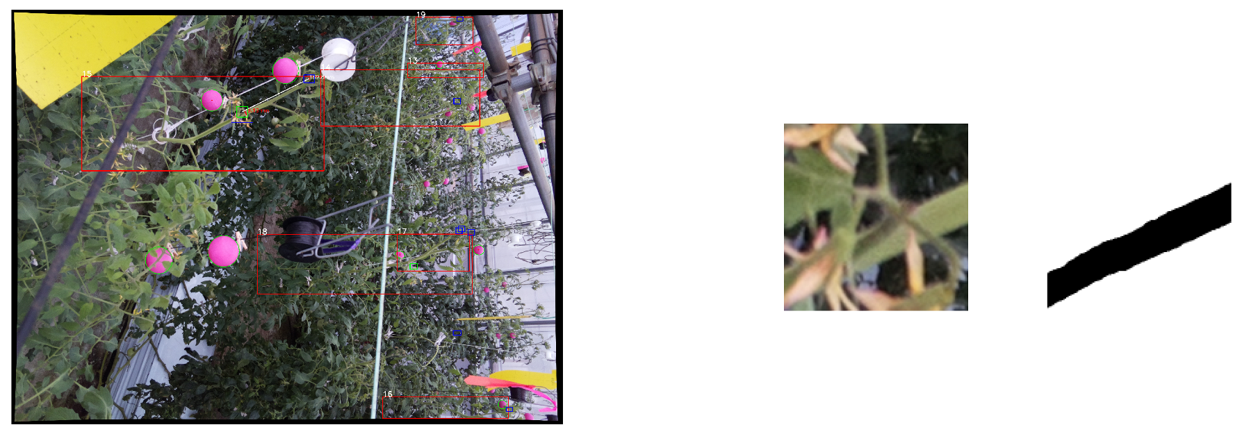
3.2.5. Stem Contour Detection Using Segmentation

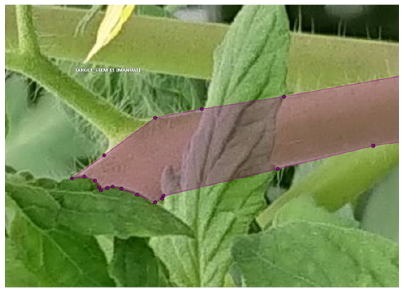
The next step is to extract the contour of the stem using DeepLabv3+, a deep learning segmentation. DeepLabv3+ is an extension of the existing DeepLabv3 called semantic segmentation which labels all pixels in an image [14]. It performs better than traditional methods such as U-Net, achieving 89% performance on the test set. We created the training data for this process. An example of an image with training data in a polygon format is shown in Figure 7. The training of DeepLabv3+ was performed with a batch size of 10 and an epoch count of 200 using Adam. No data augmentation was performed. The learning rate was set to 1 $\times {10}^{-3}$ initially and changed to 1 $\times {10}^{-4}$ after 120 epochs.

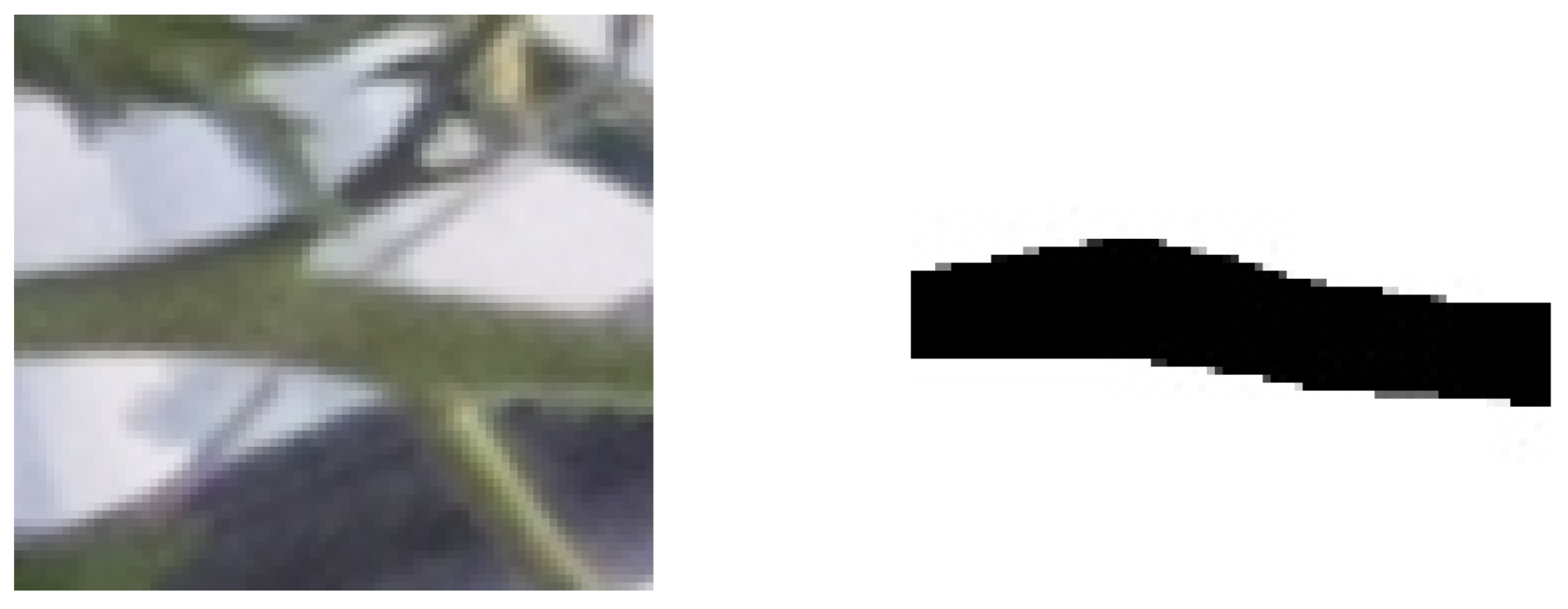
The extraction results of segmentation using DeepLabv3+ are shown in Figure 8. The black areas in the right image are the extracted stems.

Due to the complexity of measuring stem diameter from stem images obtained by YOLOv5 using traditional image processing techniques, we chose to utilize deep learning-based segmentation for obtaining stem contours. After testing and evaluating various models, we found that DeepLabv3+ offered superior detection performance in comparison to alternatives such as R-CNN and was both lightweight and suitable for our system.

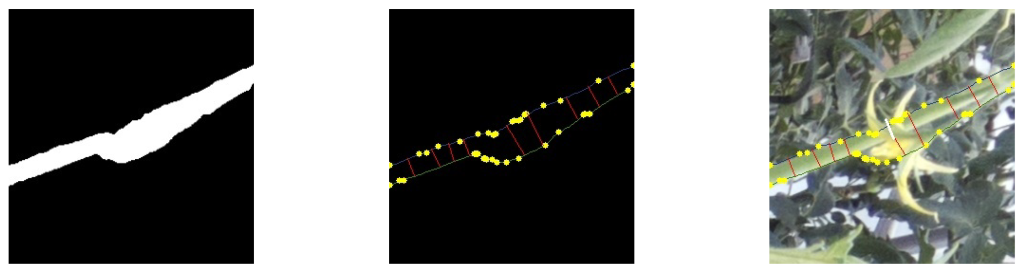
3.2.6. Measurement of Stem Diameter in Pixels

We proposed a novel method for measuring stem diameter. It involves measuring the distance between a line segment on one side edge of the stem and a line segment on the opposite side edge. We use line-to-line distance measurement instead of point-to-point distance measurement. This increases accuracy and reduces the number of inaccurate results. The process aims to obtain a set of pairs of opposite sides suitable for stem diameter measurement. The process for measuring stem diameter in pixels is outlined in the following steps:

• Apply a Gaussian filter to the binary image to suppress noise, then detect stem contours using a Laplacian filter.
• Find the contours of the stem as a continuous line connected in eight neighborhoods and list them in pixels.
• Divide the contour into two parts on both sides of the stem.
• Extract feature points using two methods to vectorize the contour.
• Vectorize feature points as endpoints and obtain contour segments of a certain length or longer as line segments.
• Calculate the stem diameters by corresponding the stem contour segments with the stem contour segments on the opposite side.
• Cluster the stem diameters of the corresponding contour segments.
• Take a weighted average and calculate the stem diameter with the length of the overlap for each cluster.
• Calculate the correctness score of the stem diameter for each cluster, and the stem diameter of the cluster with the highest score is the measured stem diameter.

In step 3, if a single contour is obtained, the contour is divided by the point farthest from the starting point of the list. Additionally, in the case of obtaining two or more contours, the longest two are obtained in terms of length (number of pixels), and the ratio of the length is taken from the one with the larger ratio to the other one when the ratio is greater than 0.7. This is because the lengths of both sides of the stem are generally similar values, and if the ratio is greatly different, there is a possibility of measuring the wrong location and it is necessary to eliminate it.

In step 4, feature points are placed at points of high curvature. Specifically, the entire stem contour is scanned, and feature points are assigned when the angle between the midpoint of the interval and the endpoints of the interval is less than a certain angle in a certain short interval. Feature points of the other type are placed at points that divide loose curves longer than a certain length. Specifically, the entire stem contour is scanned, and when the average distance between a point between two points and the line connecting the two points exceeds a certain distance, the point farthest from the line is assigned as the feature point. Together with operation in step 5, the former feature point is used to extract the appropriate stem contour by excluding parts that do not look like the stem contour. The latter feature point is intended to improve the accuracy of stem diameter measurement in the presence of loose curves.

In step 5, contour segments of greater than a certain length are vectorized by projecting the endpoints on the line with the smallest sum of the squared distances.

In step 6, a distance between the line segments is calculated by a unique method and used as the stem diameter. Two segments of the stem contour are taken from each side and normalized to obtain two direction vectors. From the two direction vectors, we calculate the mean vector and the vector orthogonal to it. The segments of the stem contour are projected onto the mean vector, and when there is overlap and the angle formed by the two original vectors is less than a certain angle (the segments of the two contours are almost parallel), it is considered that the segments of the stem contour correspond to each other. One segment of the stem contour is taken from each side and normalized to obtain two direction vectors and their mean vector. If the two stem contour segments overlap when projected onto the mean vector and the angle formed by the two original vectors is smaller than a certain angle (the two contour segments are nearly parallel), the stem contour segments are considered to correspond to each other. A straight line passes through the center of the region where the two projected contour segments overlap and, perpendicular to the mean vector, intersects the two stem contour segments, which have two intersections each.

The distance between the two intersecting points is calculated as the stem diameter of the corresponding two contour segments.

In step 7, we cluster the obtained multiple stem diameters by using the fact that the stem diameter does not change significantly (within ± about 17%). This separates clusters of correct stem diameter and incorrect stem diameter.

In step 8, the weighted average of the stem diameter is taken for each cluster, with the length of the overlap when projected as a weight.

In step 9, correct stem contours have longer overlaps and are often calculated shorter than in the case of errors. The stem diameter correctness score is calculated as (overlap length)/(stem contour length), and the stem diameter of the cluster with the highest score is considered the measured stem diameter.

The process for extracting the stem diameter is shown in Figure 9.

3.2.7. Calculation of Measurement with Reference Ball

The next step is to calculate the stem diameter and length from the base of the flower cluster to the growing point from nearby reference balls. We use the reference ball with the closest Euclidean distance on the image from the labels ‘target stem’ and ‘seichouten’.

To calculate the actual stem diameter $d_{mm}$ mm from the stem diameter $d_{px}$ px on the image and the diameter of the reference ball $r_{px}$ px, we use Formula (1). $r_{mm}$ mm is the diameter of the reference ball, which is 40 mm in our experiment. The $\alpha$ is the value calculated by the experiment, which is 1.2 in our system.

$$d_{mm}=\alpha \frac{r_{mm}}{r_{px}}{d}_{px}$$

(1)

To find the distance between the vegetative part and stem at the base of the flower cluster, we first calculate the Euclidean distance $d_{px}$ px between the ‘target stem’ and ‘seichouten’ in the image. Then, we calculate the angle $\theta$ between the ‘target stem’, camera, and ‘seichouten’ in 3D coordinates from the image using Formula (2), where W is the number of pixels in the width of the captured image and $V_W$ is the angle of view of the camera.

$$\theta =\frac{d_{px}}{W}{V}_W$$

(2)

Then, using the reference ball, we calculate the distance l mm between the camera and target using Formula (3).

$$l=\frac{r_{mm}}{r_{px}}\frac{W}{2tan\frac{V_W}{2}}$$

(3)

From Equation (3), we calculate distances $l_t$ and $l_s$ from the camera using the reference balls corresponding to ‘target stem’ and ‘seichouten’. Finally, we calculate the distance between the growing point and stem at the base of the flower cluster, $S_{mm}$ mm, using the cosine theorem and Equation (4).

$$S_{mm}=\sqrt{l_t^2+l_s^2-2l_t{l}_{s}cos\theta }$$

(4)

From these equations, the stem diameter and distance between the vegetative part and stem at the base of the flowering cluster can be calculated from the image.

3.2.8. Conversion of Measurement Data to CSV Format

Finally, the calculated stem diameters and distances between the vegetative part and stem at the base of the flower cluster are summarized in the CSV format. In this process, four pieces of information are included: the time of shooting, the ID assigned to the plant, the stem diameter, and the distance between the vegetative part and the base of the flower cluster. The ID assigned to a plant is the number assigned to the stem when determining the identity of the plant, and the same ID is assigned to plants that are determined to be the same in images taken at different locations, times, and angles.

3.3. Output of Image Analysis

A camera device is installed in the field, image analysis is performed on the captured images, and the data are compiled in CSV format. The CSV file contains data measured from the plants detected by a single camera on a single day. Therefore, CSV files are created for the number of cameras uploaded to Google Drive within a day. If the stem diameter can be measured even when the vegetative part cannot be detected, the measurement result of the distance between the vegetative part and stem at the base of the flower cluster is output as −1. The reason for this is that it is difficult to detect the growing point, and some growth analysis is possible only with stem diameter information.

4. Experimental Evaluation

4.1. Evaluation Method

Using this system, pictures were captured in a plastic greenhouse. The stem contour and size of the reference ball were obtained from the image. The relative error was calculated by comparing the result of the stem thickness calculation with the value measured by a measuring instrument, such as a caliper. The stems to be evaluated were only those to which the reference ball was attached and the stem diameter was calculated by this system. We also evaluated the detection results of YOLOv5, YOLOv4, Scaled-YOLOv4, and DeepLabv3+ and compared YOLOv5 with YOLOv4 and Scaled-YOLOv4 [15]

4.2. Results

Table 3. Detection results of each label by YOLOv5.

Label	Precision	Recall	F-Measure
stem	0.720	0.454	0.557
target stem	0.676	0.333	0.446
growing point	0.387	0.257	0.309
mean	0.594	0.348	0.437

,

Table 4. Detection results of each label by YOLOv4.

Label	Precision	Recall	F-Measure
stem	0.559	0.410	0.464
target stem	0.591	0.333	0.426
growing point	0.326	0.203	0.250
mean	0.492	0.315	0.38

and

Table 5. Detection results of each label by Scaled-YOLOv4.

Label	Precision	Recall	F-Measure
stem	0.629	0.513	0.565
target stem	0.750	0.308	0.436
growing point	0.455	0.203	0.280
mean	0.611	0.457	0.427

show the results of detecting each label by the YOLOv5, YOLOv4, and Scaled-YOLOv4, respectively, from the collected image data. This includes the same tomato plants taken at different times and from different angles.

These detection results indicated that YOLOv4 was inferior to YOLOv5 on all indicators. Although Scaled-YOLOv4 is superior to YOLOv5 in the precision and recall averages, it is inferior to YOLOv5 in the F-measure, which is an overall index.

Table 6. Evaluation of errors in stem diameter.

Stem	Measured Value [mm]	Calculation Result [mm]	Relative Error [%]
1	9.7	8.93	7.9
2	8.3	8.08	2.7
3	8.7	9.19	5.6

shows the results of calculating the relative error from the values measured by the measuring instruments based on the results of successfully detecting the reference ball and extracting the stem contour from the images taken from the plant.

The images from which the stem diameter could be calculated, the image extracted by YOLOv5, and the image of the stem contour discriminated by DeepLabv3+ are shown in Figure 10, Figure 11 and Figure 12. The detection result of stems by YOLO is indicated by a red bounding box, the detection result of the target stem is indicated by a green bounding box, and the detection result of the growing point is indicated by a blue bounding box.

The system was able to detect stems and stem outlines using YOLOv5 and a reference ball around the stem. The number of tomato plants included in the images taken over three days was 31, of which 7 were measurable stems. Therefore, the detection rate of measurable plants was 23%.

5. Discussion

In this research, it was found that if the plant to be measured and the ball attached to it can be detected correctly in the image, the stem diameter can be calculated with an error of less than 10%. Owing to the characteristics of the camera lens, it was difficult to measure the stem diameter correctly when the stem is detected at the edge of the image due to image distortion. After changing the orientation of the camera so that the detected stem is in the center of the image, the measurement can be performed with less error.

The camera device developed in this study cost about USD 150 each, and once installed, it does not need to be moved unless they malfunction. This is a significant cost saving as commercially available stem diameter change sensors cost USD 780 to USD 3900 per plant [16]. The reference balls need to be attached to each plant, one on each stem near the tomato flower cluster and one near the growing point, and the tomatoes grow so fast that they need to be moved once every two weeks. The work involved in this system requires only moving the reference balls once every two weeks, and can be done in less time than measuring tomato stems with calipers. This work can also be done at the same time if the plants are being cultivated with attractant cords. In this experiment, it took about 5 min per 10 plants to change the position of the reference ball. This method takes about 80% less time than the method using calipers, and there is no possibility of damaging the stems. This method can greatly reduce the user’s labor.

However, the system developed in this research has difficulty in detecting tomato plants by machine learning when the distance between the camera and the target tomatoes is large, or when the angle of the camera changes. Therefore, the number of plants that could be detected was reduced. Future issues include improving the detection performance of machine learning. We also believe that the use of a camera with an autofocus function as a hardware improvement will make it possible to measure plants at greater distances.