A Comparative Study for Control of Quadrotor UAVs

Abstract

Modeling and controlling highly nonlinear, multivariable, unstable, coupled and underactuated systems are challenging problems to which a unique solution does not exist. Modeling and control of Unmanned Aerial Vehicles (UAVs) with four rotors fall into that category of problems. In this paper, a nonlinear quadrotor UAV dynamical model is developed with the Newton–Euler method, and a control architecture is proposed for 3D trajectory tracking. The controller design is decoupled into two parts: an inner loop for attitude stabilization and an outer loop for trajectory tracking. A few attitude stabilization methods are discussed, implemented and compared, considering the following control approaches: Proportional–Integral–Derivative (PID), Linear–Quadratic Regulator (LQR), Model Predictive Control (MPC), Feedback Linearization (FL) and Sliding Mode Control (SMC). This paper is intended to serve as a guideline work for selecting quadcopters’ control strategies, both in terms of quantitative and qualitative considerations. PID and LQR controllers are designed, exploiting the model linearized about the hovering condition, while MPC, FL and SMC directly exploit the nonlinear model, with minor simplifications. The fast dynamics ensured by the SMC-based controller together with its robustness and the limited estimated command effort of the controller make it the most promising controller for quadrotor attitude stabilization. The outer loop consists of three independent PID controllers: one for altitude control and the other two, together with a dynamics’ inversion, are entitled to the computation of the reference attitude for the inner loop. The capability of the controlled closed-loop system of executing complex trajectories is demonstrated by means of simulations in MATLAB/Simulink^®.

1. Introduction

The growth of the number of applications of Unmanned Aerial Vehicles (UAVs) in many different fields, from civilian to military applications, has experienced a big rise over the last decade. As highlighted in specific literature reviews [1,2], the civilian applications of UAVs include activities such as parcel delivery, transportation of medical samples, mapping, surveillance, precision agriculture and greenhouses [3], population health monitoring, disaster recovery, personal use and photography, to name a few. The advantages due to the adoption of UAVs in each application domain have been widely reviewed. Just to give an example, considering the logistic domain discussed in [4], UAVs can contribute to optimizing the logistic process, reducing resources’ usage, traffic and CO₂ emissions, inducing the diversification of transportation options as well as giving rise to new business models.

Therefore, UAVs have gained significant interest from the engineering research world over the last two decades. In particular, quadrotors are the most researched and used type of UAVs because of their mechanical structure, which is relatively simple to model, their enhanced closed-loop stability with respect to other configurations and their high maneuverability in both indoor and outdoor spaces, as described in [5]. However, quadcopters are mechatronic systems with nonlinear, multivariable, unstable, coupled and underactuated characteristics, which make the control not trivial.

Literature reviews such as [6,7,8,9] provide a comprehensive analysis of the main state-of-the-art control strategies for quadrotor UAVs. The well-known Proportional–Integral–Derivative (PID) control can effectively handle both linear and nonlinear systems. This is because it is model-independent and has a simple-to-understand tuning principle. Additionally, PID control can achieve zero steady-state error. On the other hand, PID control cannot handle constraints, is poorly robust with respect to disturbances and uncertainties and may require extensive tuning. The research in [10] implements a quadrotor attitude controller by means of a PID controller optimized with a genetic algorithm.

The Linear–Quadratic Regulator (LQR) control approach is equivalent to solving an optimization problem, with the cost function weighted of the squared norms of tracking error and control input signals, under the constraint of satisfying the system’s dynamics. It is designed with a linear approximation of the system and may not guarantee a zero steady-state error. LQR control can find an optimal feedback gain matrix considering both the tracking performances and the command input effort of the controller.

The Feedback Linearization (FL) control approach consists of a systematic procedure to linearize the system with a model inversion and control it with a new control input term. The system is transformed into a linear system without any linearization assumption and can be controlled according to the linear control theory. FL performs well when the nonlinear plant is similar to the one used for control design, so it is not very robust to parametric uncertainties and cannot handle constraints. A feedback linearization attitude controller with proportional action is proposed in [11].

The Sliding Mode Control (SMC) approach aims at bringing the system state to the “sliding surface”, which is a subset of the state space that corresponds to a desired dynamical behavior. The control law is the sum of a continuous function of the system’s state and the reference, which guarantees that the “sliding surface” is invariant (once the state is on the sliding surface, it remains on it), and a discontinuous term for convergence to the “sliding surface”. SMC shows, in general, good robustness to model uncertainties and disturbances, but a smooth approximation of the control law is necessary to avoid chattering, which may lead to instability.

The Model Predictive Control (MPC) approach solves an optimization problem at each defined time step to compute the optimal control input, satisfying the system’s dynamics, input and state constraints. A prediction model is exploited to predict the future states of the system. MPC is quite robust to disturbances but may be slow in tracking. The MPC-based position trajectory controller designed in [12], despite exploiting a linear model for prediction, shows the ability to ensure tracking of complex trajectories.

Furthermore, other control laws can be effectively applied to quadrotors, such as H-infinity, Backstepping, Adaptive, Fuzzy and Neural Network control. A Backstepping controller for position control of a quadrotor helicopter is designed and validated in [13], with stability being proven by the Lyapunov method. Additionally, a Fuzzy Logic controller for attitude control has been proposed in [14]. An L₁ adaptive controller is designed and validated in [15] for the attitude controller of a mini-UAV. Adaptive control does not need a parameter tuning procedure and deals with parametric uncertainties and unmodelled dynamics. The Sliding Mode-based adaptive controller with Proportional–Integral–Derivative gains proposed in [16] controls a micro-UAV, the Parrot Mambo Minidrone, and is demonstrated on a model-based platform. In [17], an adaptive controller is proven to be able to deal with parametric uncertainties and external disturbances and performs well with unknown time delays inserted in the closed-loop dynamics.

In this paper, a comparative study of 3D trajectory control of a quadrotor system is proposed. The control system is decoupled into an outer loop for trajectory control and an inner loop for attitude control; input saturation is also taken into account. Despite several reviews of control algorithms for quadrotors being proposed in the literature, such as [6,7,8,9] to state a few, there is, to the best extent of our knowledge, poor availability of comparative studies where several approaches are implemented and discussed. The comparative study proposed in [18] implements PID, LQR, Fuzzy and Adaptive controllers for position trajectory tracking, while PID, LQR and MPC-based attitude stabilizers are implemented and discussed in [19]. In order to enlarge the available state of the art of quantitative comparative performance evaluation for quadrotors’ control, we propose a broad comparative implementation of different control approaches (PID, LQR, MPC, FL and SMC) to the quadrotor attitude stabilization problem. Linearized or simplified attitude dynamical systems are exploited in the design phase, yet all the controllers are tested with the proposed full nonlinear model. According to the fast dynamic response, the robustness to the discrepancy between the control model and the full nonlinear model and an approximative L₂ norm-based trade-off evaluation of both the tracking performance and the command effort of the controller, the most suitable method is selected for the inner loop control part of the complete proposed control architecture. The outer loop is designed to track velocity references by exploiting PID control and a dynamics inversion from a simplified translational dynamical model.

This paper is organized as follows. The system model derived with the Newton–Euler formalism is reported in Section 2, as well as the proposed control system architecture, the proposed control laws and the simulation parameters setting. Section 3 presents the simulation results in which a micro-UAV is demonstrated to be able to execute complex trajectories with the complete control system. Conclusions and future research directions are drawn in Section 4.

2. Materials and Methods

2.1. System Model

Quadrotor UAVs are mechatronic systems with two rigid arms arranged in a cross configuration and four rotors. Each pair of rotors is located at the arm’s extremity and rotates in opposite directions. The speed of the rotors is controlled independently. A picture of a commercial quadrotor platform is shown in Figure 1. The movement of flying quadrotors derives from the total lift force produced by all rotors and from their capability of inclination, which is due to the resultant forces acting on the arms and to the resultant counter-torque caused by the pairs of rotors. The representation shown in Figure 2 is derived from the configuration of Figure 1, considered as a reference for the formulation of the quadrotor dynamical model.

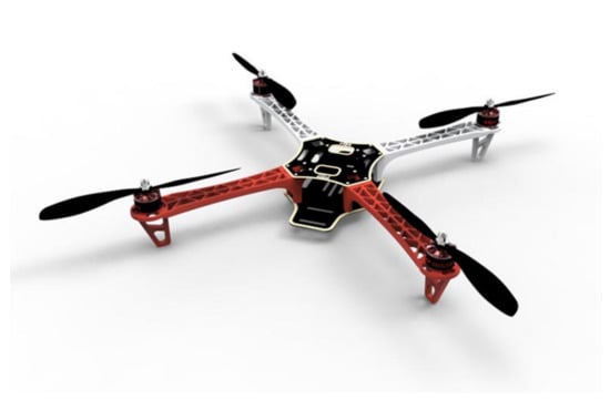
Figure 1. Picture of a commercial quadcopter platform [20].

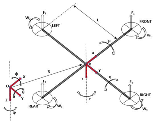
Figure 2. Schematic representation of the quadrotor configuration of reference.

Two reference frames are defined in order to characterize the position and the orientation of the UAV: a fixed inertial reference frame $\mathrm{OXYZ}$ and a body reference frame $\mathrm{oxyz}$ attached to the quadrotor. The relation between the two is expressed by the homogeneous transformation matrix $T_L$ derived with the Euler ZYX convention, also known as the RPY convention. The RPY convention involves three rotations. Firstly, a rotation of $\mathsf{\psi }$ (Euler yaw angle) about $\mathrm{Z}$ produces the frame ${\mathrm{OX}}_1{\mathrm{Y}}_1\mathrm{Z}$. Secondly, a second rotation of $\mathsf{\vartheta }$ (Euler pitch angle) about ${\mathrm{Y}}_1$ results in the frame ${\mathrm{OX}}_2{\mathrm{Y}}_1{\mathrm{Z}}_1$. Lastly, a third rotation of $\mathsf{\varphi }$ (Euler roll angle) about ${\mathrm{X}}_2$ results in the frame ${\mathrm{OX}}_2{\mathrm{Y}}_2{\mathrm{Z}}_2$ (coincident with $\mathrm{oxyz}$). These rotations are performed according to a post multiplication rule,

$$T_L=T_{\psi }{T}_{\theta }{T}_{\mathsf{\varphi }}=\left(\begin{array}{ccc}{\mathrm{c}}_{\mathsf{\psi }}& -{\mathrm{s}}_{\mathsf{\psi }}& 0\\ {\mathrm{s}}_{\mathsf{\psi }}& {\mathrm{c}}_{\mathsf{\psi }}& 0\\ 0& 0& 1\end{array}\right)\left(\begin{array}{ccc}{\mathrm{c}}_{\mathsf{\theta }}& 0& {\mathrm{s}}_{\mathsf{\theta }}\\ 0& 1& 0\\ -{\mathrm{s}}_{\mathsf{\theta }}& 0& {\mathrm{c}}_{\mathsf{\theta }}\end{array}\right)\left(\begin{array}{ccc}1& 0& 0\\ 0& {\mathrm{c}}_{\mathsf{\varphi }}& -{\mathrm{s}}_{\mathsf{\varphi }}\\ 0& {\mathrm{s}}_{\mathsf{\varphi }}& {\mathrm{c}}_{\mathsf{\varphi }}\end{array}\right) =\left(\begin{array}{ccc}{\mathrm{c}}_{\mathsf{\psi }}{\mathrm{c}}_{\mathsf{\theta }}& {\mathrm{c}}_{\mathsf{\psi }}{\mathrm{s}}_{\mathsf{\theta }}{\mathrm{s}}_{\mathsf{\varphi }}-{\mathrm{s}}_{\mathsf{\psi }}{\mathrm{c}}_{\mathsf{\varphi }}& {\mathrm{s}}_{\mathsf{\psi }}{\mathrm{s}}_{\mathsf{\varphi }}+{\mathrm{c}}_{\mathsf{\psi }}{\mathrm{s}}_{\mathsf{\theta }}{\mathrm{c}}_{\mathsf{\varphi }}\\ {\mathrm{s}}_{\mathsf{\psi }}{\mathrm{c}}_{\mathsf{\theta }}& {\mathrm{c}}_{\mathsf{\psi }}{\mathrm{c}}_{\mathsf{\varphi }}+{\mathrm{s}}_{\mathsf{\theta }}{\mathrm{s}}_{\mathsf{\psi }}{\mathrm{s}}_{\mathsf{\varphi }}& {\mathrm{s}}_{\mathsf{\theta }}{\mathrm{s}}_{\mathsf{\psi }}{\mathrm{c}}_{\mathsf{\varphi }}-{\mathrm{s}}_{\mathsf{\varphi }}{\mathrm{c}}_{\mathsf{\psi }}\\ -{\mathrm{s}}_{\mathsf{\theta }}& {\mathrm{c}}_{\mathsf{\theta }}{\mathrm{s}}_{\mathsf{\varphi }}& {\mathrm{c}}_{\mathsf{\theta }}{\mathrm{c}}_{\mathsf{\varphi }}\end{array}\right)$$

(1)

where $\mathrm{c}$ and $\mathrm{s}$ denote cosine and sine functions, respectively. $T_L$ transforms linear movement-related vectors from $\mathrm{oxyz}$ to $\mathrm{OXYZ}$. Consequently, $T_R$ transforms rotational movement-related vectors from $\mathrm{OXYZ}$ to $\mathrm{oxyz}$,

$$\Delta =\left(\begin{array}{c}\mathrm{p}\\ \mathrm{q}\\ \mathrm{r}\end{array}\right)=T_{\mathsf{\varphi }}^T\left(\begin{array}{c}{\mathsf{\varphi }}^{\prime }\\ 0\\ 0\end{array}\right)+T_{\mathsf{\varphi }}^T{T}_{\theta }^T\left(\begin{array}{c}0\\ {\mathsf{\theta }}^{\prime }\\ 0\end{array}\right)+T_{\mathsf{\varphi }}^T{T}_{\theta }^T{T}_{\psi }^T\left(\begin{array}{c}0\\ 0\\ {\mathsf{\psi }}^{\prime }\end{array}\right)=\left(\begin{array}{ccc}1& 0& -{\mathrm{s}}_{\mathsf{\theta }}\\ 0& {\mathrm{c}}_{\mathsf{\varphi }}& {\mathrm{c}}_{\mathsf{\theta }}{\mathrm{s}}_{\mathsf{\varphi }}\\ 0& -{\mathrm{s}}_{\mathsf{\varphi }}& {\mathrm{c}}_{\mathsf{\theta }}{\mathrm{c}}_{\mathsf{\varphi }}\end{array}\right)\left(\begin{array}{c}{\mathsf{\varphi }}^{\prime }\\ {\mathsf{\theta }}^{\prime }\\ {\mathsf{\psi }}^{\prime }\end{array}\right)=T_R\left(\begin{array}{c}{\mathsf{\varphi }}^{\prime }\\ {\mathsf{\theta }}^{\prime }\\ {\mathsf{\psi }}^{\prime }\end{array}\right)$$

(2)

where $\mathrm{p}$, $\mathrm{q}$ and $\mathrm{r}$ denote the rotational velocities in the body frame, while ${\mathsf{\varphi }}^{\prime }$, ${\vartheta }^{\prime }$ and ${\mathsf{\psi }}^{\prime }$ denote the Euler rates. The Newton–Euler formalism is adopted to present the quadrotor dynamical model; for further details about modeling refer to [21,22,23,24].

In the adopted model, the following assumptions are made:

• The structure is perfectly symmetrical.
• The structure is perfectly symmetrical.
• The structure is perfectly rigid.
• The quadrotor’s center of mass coincides with the origin of the body fixed frame.
• The rotors’ motors dynamics are neglected.
• Complex phenomena of difficult modeling are neglected, such as the ground effect, blade flapping and any other minor aerodynamical or inertial contributions not explicitly taken into account.

It follows the translational dynamical model in the inertial fixed reference frame,

$$\mathrm{m}{R}^{″}=\mathrm{m}g-{\mathrm{K}}_{\mathrm{d}}^{\mathrm{L}}{R}^{\prime }-\left(F_1+F_2+F_3+F_4\right)T_L$$

(3)

$$F_i=\left(\begin{array}{c}0\\ 0\\ {\mathrm{bw}}_{\mathrm{i}}^2\end{array}\right) , \mathrm{with} \mathrm{i}=1,2,3,4$$

(4)

where $R$ denotes the position vector in $\mathrm{OXYZ}$, $F_i$ is the thrust force produced by rotor $\mathrm{i}$, ${\mathrm{w}}_{\mathrm{i}}$ is the angular speed of rotor $\mathrm{i}$, $\mathrm{b}$ is the thrust coefficient, $\mathrm{m}$ is the quadcopter’s mass, $g$ is the gravity acceleration and ${\mathrm{K}}_{\mathrm{d}}^{\mathrm{L}}$ denotes the aerodynamic thrust drag coefficient. It follows the rotational dynamical model in the body reference frame,

$$\mathrm{I}{\Delta }^{\prime }=-\left(\Delta \mathrm{x} \mathrm{I}\Delta \right)-M_{gy}-{\mathrm{K}}_{\mathrm{d}}^{\mathrm{R}}\Delta +M$$

(5)

$$M_{gy}={\mathrm{I}}_{\mathrm{R}}\left({\mathrm{w}}_1+{\mathrm{w}}_3-{\mathrm{w}}_2-{\mathrm{w}}_4\right) \Delta \times \left(\begin{array}{c}0\\ 0\\ 1\end{array}\right)$$

(6)

$$M=\left(\begin{array}{c}\mathrm{L}({\mathrm{F}}_2-{\mathrm{F}}_4)\\ \mathrm{L}({\mathrm{F}}_1-{\mathrm{F}}_3)\\ \mathsf{d}\left({\mathrm{w}}_1^2-{\mathrm{w}}_2^2+{\mathrm{w}}_3^2-{\mathrm{w}}_4^2\right)\end{array}\right)$$

(7)

$$\mathrm{I}=\left(\begin{array}{ccc}{\mathrm{I}}_{\mathrm{x}}& 0& 0\\ 0& {\mathrm{I}}_{\mathrm{y}}& 0\\ 0& 0& {\mathrm{I}}_{\mathrm{z}}\end{array}\right)$$

(8)

with the quadrotor’s arm length being $\mathrm{L}$, the diagonal inertia matrix $\mathrm{I}$, the inertia of the rotors ${\mathrm{I}}_{\mathrm{R}}$, the drag coefficient $\mathrm{d}$, the aerodynamic moment drag coefficient ${\mathrm{K}}_{\mathrm{d}}^{\mathrm{R}}$, the rotors’ induced moment vector $M$ and the gyroscopic moment vector $M_{gy}$; the latter is due to the fact that the axes of rotation of the propellers are attached to the quadrotor and rotate with it. The complete nonlinear dynamical model of the quadrotor is derived by evaluating Equations (3) and (5) and considering the transformations in Equations (1) and (2):

$${\mathrm{X}}^{″}=-\frac{1}{\mathrm{m}}{\mathrm{K}}_{\mathrm{d}}^{\mathrm{L}}{\mathrm{X}}^{\prime }-\frac{1}{\mathrm{m}}\left({\mathrm{s}}_{\mathsf{\psi }}{\mathrm{s}}_{\mathsf{\varphi }}+{\mathrm{c}}_{\mathsf{\psi }}{\mathrm{s}}_{\mathsf{\theta }}{\mathrm{c}}_{\mathsf{\varphi }}\right){\mathrm{U}}_1$$

(9)

$${\mathrm{Y}}^{″}=-\frac{1}{\mathrm{m}}{\mathrm{K}}_{\mathrm{d}}^{\mathrm{L}}{\mathrm{Y}}^{\prime }-\frac{1}{\mathrm{m}}\left({\mathrm{s}}_{\mathsf{\theta }}{\mathrm{s}}_{\mathsf{\psi }}{\mathrm{c}}_{\mathsf{\varphi }}-{\mathrm{s}}_{\mathsf{\varphi }}{\mathrm{c}}_{\mathsf{\psi }}\right){\mathrm{U}}_1$$

(10)

$${\mathrm{Z}}^{″}=\mathrm{g}-\frac{1}{\mathrm{m}}{\mathrm{K}}_{\mathrm{d}}^{\mathrm{L}}{\mathrm{Z}}^{\prime }-\frac{1}{\mathrm{m}}{\mathrm{c}}_{\mathsf{\theta }}{\mathrm{c}}_{\mathsf{\varphi }}{\mathrm{U}}_1$$

(11)

$${\mathrm{p}}^{\prime }=\frac{{\mathrm{I}}_{\mathrm{Y}}-{\mathrm{I}}_{\mathrm{z}}}{{\mathrm{I}}_{\mathrm{x}}}\mathrm{qr}-\frac{{\mathrm{I}}_{\mathrm{R}}}{{\mathrm{I}}_{\mathrm{x}}}\mathrm{q}\left({\mathrm{w}}_1+{\mathrm{w}}_3-{\mathrm{w}}_2-{\mathrm{w}}_4\right)-\frac{1}{{\mathrm{I}}_{\mathrm{x}}}{\mathrm{K}}_{\mathrm{d}}^{\mathrm{R}}\mathrm{p}+\frac{1}{{\mathrm{I}}_{\mathrm{x}}}{\mathrm{LU}}_2$$

(12)

$${\mathrm{q}}^{\prime }=\frac{{\mathrm{I}}_{\mathrm{z}}-{\mathrm{I}}_{\mathrm{x}}}{{\mathrm{I}}_{\mathrm{y}}}\mathrm{pr}-\frac{{\mathrm{I}}_{\mathrm{R}}}{{\mathrm{I}}_{\mathrm{y}}}\mathrm{p}\left({\mathrm{w}}_1+{\mathrm{w}}_3-{\mathrm{w}}_2-{\mathrm{w}}_4\right)-\frac{1}{{\mathrm{I}}_{\mathrm{y}}}{\mathrm{K}}_{\mathrm{d}}^{\mathrm{R}}\mathrm{q}+\frac{1}{{\mathrm{I}}_{\mathrm{y}}}{\mathrm{LU}}_3$$

(13)

$${\mathrm{r}}^{\prime }=\frac{{\mathrm{I}}_{\mathrm{x}}-{\mathrm{I}}_{\mathrm{y}}}{{\mathrm{I}}_{\mathrm{z}}}\mathrm{pq}-\frac{1}{{\mathrm{I}}_{\mathrm{z}}}{\mathrm{K}}_{\mathrm{d}}^{\mathrm{R}}\mathrm{r}+\frac{1}{{\mathrm{I}}_{\mathrm{z}}}{\mathrm{U}}_4$$

(14)

$${\mathsf{\varphi }}^{\prime }=\mathrm{p}+{\mathrm{s}}_{\mathsf{\varphi }}{\mathrm{s}}_{\mathsf{\theta }}{\mathrm{c}}_{\mathsf{\theta }}^{-1}\mathrm{q}+{\mathrm{c}}_{\mathsf{\varphi }}{\mathrm{s}}_{\mathsf{\theta }}{\mathrm{c}}_{\mathsf{\theta }}^{-1}\mathrm{r}$$

(15)

$${\mathsf{\theta }}^{\prime }={\mathrm{c}}_{\mathsf{\varphi }}\mathrm{q}-{\mathrm{s}}_{\mathsf{\varphi }}\mathrm{r}$$

(16)

$${\mathsf{\psi }}^{\prime }={\mathrm{s}}_{\mathsf{\varphi }}{\mathrm{c}}_{\mathsf{\theta }}^{-1}\mathrm{q}+{\mathrm{c}}_{\mathsf{\theta }}^{-1}{\mathrm{c}}_{\mathsf{\varphi }}\mathrm{r}$$

(17)

$$u=\left(\begin{array}{c}{\mathrm{U}}_1\\ {\mathrm{U}}_2\\ {\mathrm{U}}_3\\ {\mathrm{U}}_4\end{array}\right)={\mathrm{M}}_{\mathrm{bd}}{w}^2=\left(\begin{array}{cccc}\mathrm{b}& \mathrm{b}& \mathrm{b}& \mathrm{b}\\ 0& \mathrm{b}& 0& -\mathrm{b}\\ \mathrm{b}& 0& -\mathrm{b}& 0\\ \mathrm{d}& -\mathrm{d}& \mathrm{d}& -\mathrm{d}\end{array}\right)\left(\begin{array}{c}{\mathrm{w}}_1^2\\ {\mathrm{w}}_2^2\\ {\mathrm{w}}_3^2\\ {\mathrm{w}}_4^2\end{array}\right)$$

(18)

It is worth noting that Equation (18) stands for an artificial input transformation made for ease of representation and control law definition. ${\mathrm{U}}_1$ denotes the total lift force produced by the rotors, ${\mathrm{U}}_2$ and ${\mathrm{U}}_3$ are the resultant forces generating pitch and roll movement respectively and ${\mathrm{U}}_4$ is the resultant moment acting on the yaw axis. The presented quadrotor dynamical model has 12 state variables $x=\left({\mathrm{x}}_1,{ \mathrm{x}}_2,{ \mathrm{x}}_3,{\mathrm{x}}_4,{\mathrm{x}}_5,{\mathrm{x}}_6,{\mathrm{x}}_7,{\mathrm{x}}_8,{\mathrm{x}}_9,{\mathrm{x}}_{10},{\mathrm{x}}_{11},{ \mathrm{x}}_{12}\right)=\left(\mathrm{X},\mathrm{Y},\mathrm{Z}, {\mathrm{X}}^{\prime }, {\mathrm{Y}}^{\prime }, {\mathrm{Z}}^{\prime },\mathsf{\varphi },\mathsf{\theta },\mathsf{\psi },\mathrm{p},\mathrm{q},\mathrm{r}\right)$ and 4 input variables $u=\left({\mathrm{u}}_1,{\mathrm{u}}_2,{\mathrm{u}}_3,{\mathrm{u}}_4\right)=\left({\mathrm{U}}_1,{\mathrm{U}}_2,{\mathrm{U}}_3,{\mathrm{U}}_4\right)$. Note that the rotors’ velocities giving the gyroscopic effect contribution still appear in Equations (12) and (13) but can be rewritten as a nonlinear function of the artificial input variables $\mathrm{f}\left(u\right)$ by inversion and manipulation of Equation (18).

$$\mathrm{f}\left(u\right)={{\displaystyle \sum }}_{\mathrm{i}=1}^4{\left(-1\right)}^{\mathrm{i}+1}\sqrt{ \mid {({\mathrm{M}}_{\mathrm{bd}}{}^{-1}u)}_{\mathrm{i} }\mid }={\mathrm{w}}_1+{\mathrm{w}}_3-{\mathrm{w}}_2-{\mathrm{w}}_4$$

(19)

The system, besides presenting under-actuation characteristics that always yield to challenging control design aspects, is highly nonlinear and coupled. When dealing with a dynamical system with such properties, it is convenient to derive a linearized model in order to obtain a clearer understanding of the relation between control and state variables and the system’s stability. Furthermore, linearized models are often exploited for the design of the control law itself.

$${\mathrm{X}}^{″}=-\mathsf{\theta }\mathrm{g}$$

(20)

$${\mathrm{Y}}^{″}=-\mathsf{\varphi }\mathrm{g}$$

(21)

$${\mathrm{Z}}^{″}=\mathrm{g}-\frac{1}{\mathrm{m}}{\mathrm{U}}_1$$

(22)

$${\mathsf{\varphi }}^{″}=\frac{1}{{\mathrm{I}}_{\mathrm{x}}}{\mathrm{LU}}_2$$

(23)

$${\mathsf{\theta }}^{″}=\frac{1}{{\mathrm{I}}_{\mathrm{y}}}{\mathrm{LU}}_3$$

(24)

$${\mathsf{\psi }}^{″}=\frac{1}{{\mathrm{I}}_{\mathrm{z}}}{\mathrm{U}}_4$$

(25)

The Equations (20)–(25) refer to the linearization of the model represented by the Equations (9)–(17) by means of a Taylor expansion of the first order and adopting approximations for small angles, under the following assumptions:

• The quadrotor is hovering: external forces and moments are neglectable, linear and rotational velocities are small (the Euler rates coincide with the rotational velocities in the body frame).
• The equilibrium control input and state vectors are $\left({\mathrm{u}}_1^{\ast },{\mathrm{u}}_2^{\ast },{\mathrm{u}}_3^{\ast },{\mathrm{u}}_4^{\ast }\right)=\left(\mathrm{mg},0,0,0\right)$ and $\left({\mathrm{x}}_1,{ \mathrm{x}}_2,{ \mathrm{x}}_3,{\mathrm{x}}_4,{\mathrm{x}}_5,{\mathrm{x}}_6,{\mathrm{x}}_7,{\mathrm{x}}_8,{\mathrm{x}}_9,{\mathrm{x}}_{10},{\mathrm{x}}_{11},{ \mathrm{x}}_{12}\right)=\left(0,0,0,0,0,0,0,0,0,0,0,0\right)$, respectively.
• All terms of order higher than one are neglected.

2.2. System Control

If considering the linearized model in equations from (20) to (25) in the Laplace variable domain formulation, it is straightforward that the system is unstable due to the presence of poles in the origin. Additionally, the inputs ${\mathrm{U}}_2$, ${\mathrm{U}}_3$ and ${\mathrm{U}}_4$ directly affect the quadrotor’s attitude, while ${\mathrm{U}}_1$ directly affects the altitude dynamics. Figure 3 shows the proposed control system’s architecture, decoupled in two parts: the inner loop performs attitude stabilization, while the outer loop is responsible for altitude control and reference attitude computation, given a 3D trajectory to be followed. Each control input signal U_i is saturated before being given to the plant, i.e., the quadcopter. The lower and upper saturation bounds are ${\mathrm{U}}_{\mathrm{i}}^{\mathrm{LB}}$ and ${\mathrm{U}}_{\mathrm{i}}^{\mathrm{UB}}$, respectively. The propellers’ capacity is assumed to be such that the absolute value of the saturated total lift force ${\mathrm{U}}_1^{\mathrm{SAT}}$ is equal to $3 \mathrm{mg}$. Analogously, an absolute value of $1.5 \mathrm{mg}$ refers to ${\mathrm{U}}_2^{\mathrm{SAT}}$ and ${\mathrm{U}}_3^{\mathrm{SAT}}$, while an absolute value equal to $\mathrm{mgL}$ refers to ${\mathrm{U}}_4^{\mathrm{SAT}}$.

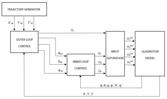
Figure 3. Overview of the proposed control system’s architecture.

The inner loop is intended to be sufficiently faster than the outer loop so that the UAV’s attitude can be effectively stabilized. Additionally, the state variables are assumed to be perfectly known to the controllers at each sampling instant. On the other hand, it is well known that the accuracy of position estimates may not be high enough to implement position-based trajectory controllers in many real-world applications. Consequently, the outer loop is intended to ensure tracking of velocity references.

As far as the inner loop is concerned, the choice of the best control law derives from a comparative evaluation of different linear and nonlinear controllers designed for attitude stabilization: PID, LQR, FL, SM and MPC. Both the tracking error and the controller command effort related to each controller are taken into account by means of the sum of the L₂ norms of state and controller command input signals. Each attitude stabilization controller is designed with simplified models but is applied to the complete nonlinear attitude system expressed by Equations (12) to (17) for the sake of the evaluation. Instead, the outer loop implements a dynamic inversion and PID-based velocity controller.

2.2.1. Inner Loop—PID Control

This follows the linearized attitude dynamical system expressed by equations from (23) to (25) in state space form, with $x=\left(\mathsf{\varphi },\mathsf{\theta },\mathsf{\psi },{\mathsf{\varphi }}^{\prime }, {\mathsf{\theta }}^{\prime }, {\mathsf{\psi }}^{\prime }\right)$ and $u=\left({\mathrm{U}}_2,{\mathrm{U}}_3,{\mathrm{U}}_4\right)$. Three independent Proportional–Integral–Derivative controllers are designed with the aim of stabilizing the linearized system in hovering.

$$\left\{\begin{array}{c}\dot{x}=\mathrm{A}x+\mathrm{B}u\\ y=\mathrm{C}x+\mathrm{D}u\end{array} \right\}$$

(26)

$$\mathrm{A}=\left(\begin{array}{cccccc}0& 0& 0& 1& 0& 0\\ 0& 0& 0& 0& 1& 0\\ 0& 0& 0& 0& 0& 1\\ 0& 0& 0& 0& 0& 0\\ 0& 0& 0& 0& 0& 0\\ 0& 0& 0& 0& 0& 0\end{array}\right) , \mathrm{B}=\left(\begin{array}{ccc}0& 0& 0\\ 0& 0& 0\\ 0& 0& 0\\ {\mathrm{LI}}_{\mathrm{x}}^{-1}& 0& 0\\ 0& {\mathrm{LI}}_{\mathrm{y}}^{-1}& 0\\ 0& 0& {\mathrm{I}}_{\mathrm{z}}^{-1}\end{array}\right) , \mathrm{C}=\left(\begin{array}{cccccc}1& 0& 0& 0& 0& 0\\ 0& 1& 0& 0& 0& 0\\ 0& 0& 1& 0& 0& 0\\ 0& 0& 0& 0& 0& 0\\ 0& 0& 0& 0& 0& 0\\ 0& 0& 0& 0& 0& 0\end{array}\right) , \mathrm{D}=\left(\begin{array}{ccc}0& 0& 0\\ 0& 0& 0\\ 0& 0& 0\end{array}\right)$$

A classical formulation of the PID control law applied to the quadrotor stabilization problem in the time domain is presented in Equation (27). The three control parameters (${\mathrm{K}}_{\mathrm{p}}^{\mathrm{i}}$,${\mathrm{K}}_{\mathrm{i}}^{\mathrm{i}}$,${\mathrm{K}}_{\mathrm{d}}^{\mathrm{i}}$) of each control command are set in order to stabilize the model in (26) for the hovering equilibrium point. Refer to [25] for the theoretical foundations of PID control and further details.

$${\mathrm{u}}^{\mathrm{p}}\left(\mathsf{t}\right)={\mathrm{u}}_{\mathrm{eq}}^{\mathrm{p}}-{\mathrm{K}}_{\mathrm{p}}^{\mathrm{p}}\left({\mathrm{y}}^{\mathrm{p}}\left(\mathsf{t}\right)-{\mathrm{y}}_{\mathrm{eq}}^{\mathrm{p}}\right)-{\mathrm{K}}_{\mathrm{i}}^{\mathrm{p}}{{\displaystyle \int }}_0^{\mathrm{T}}\left({\mathrm{y}}^{\mathrm{p}}\left(\mathsf{t}\right)-{\mathrm{y}}_{\mathrm{eq}}^{\mathrm{p}}\right)\mathrm{dt}-{\mathrm{K}}_{\mathrm{d}}^{\mathrm{p}}\left({ \dot{\mathrm{y}}}^{\mathrm{p}}\left(\mathsf{t}\right)-{ \dot{\mathrm{y}}}_{\mathrm{eq}}^{\mathrm{p}}\right) ,{\mathrm{u}}_{\mathrm{eq}}={ \mathrm{y}}_{\mathrm{eq}}=\left(0,0,0\right) , \mathrm{p}=1,2,3$$

(27)

2.2.2. Inner Loop—LQR Control

The linearized attitude dynamical model in (26) is exploited to design the LQR-based attitude stabilizer. LQR controllers are based on optimization (minimization) of the sum of the weighted energies (L₂ norms) of the state and the control command, with the constraints that the system dynamics are respected. According to the Linear–Quadratic Regulator method, since the linearized system is completely controllable, i.e., the controllability matrix has full rank, it is possible to define the following feedback control action,

$$u\left(\mathsf{t}\right)=-\mathrm{K}x\left(\mathsf{t}\right)$$

(28)

$$\mathrm{K}={\mathrm{R}}^{-1}{\mathrm{B}}^{\mathrm{T}}\mathrm{P}$$

(29)

$${\mathrm{A}}^{\mathrm{T}}\mathrm{P}+\mathrm{Q}+\mathrm{PA}-{\mathrm{PBR}}^{-1}{\mathrm{B}}^{\mathrm{T}}\mathrm{P}=0$$

(30)

$$\mathrm{Q}=\left(\begin{array}{cccccc}{\mathrm{q}}_1& 0& 0& 0& 0& 0\\ 0& {\mathrm{q}}_2& 0& 0& 0& 0\\ 0& 0& {\mathrm{q}}_3& 0& 0& 0\\ 0& 0& 0& {\mathrm{q}}_4& 0& 0\\ 0& 0& 0& 0& {\mathrm{q}}_5& 0\\ 0& 0& 0& 0& 0& {\mathrm{q}}_6\end{array}\right) , \mathrm{R}=\left(\begin{array}{ccc}{\mathrm{r}}_1& 0& 0\\ 0& {\mathrm{r}}_2& 0\\ 0& 0& {\mathrm{r}}_3\end{array}\right)$$

(31)

where $\mathrm{K}$ denotes the feedback control gain, $\mathrm{Q}$ and $\mathrm{R}$ are diagonal fixed weight matrices for the weighted L₂ norms of $x$ and $u$, respectively. The dynamics of the closed-loop system depend on the relative values of the control parameters: ${\mathrm{q}}_{\mathrm{i}}$, ${\mathrm{r}}_{\mathrm{i}}$. $\mathrm{P}$ can be computed by solving the Algebraic Riccati Equation formulated in Equation (30). Refer to [26] for the theoretical foundations of LQR control and further details.

2.2.3. Inner Loop—Feedback Linearization Control

This follows the attitude dynamical system exploited for the design of the feedback linearization-based attitude controller, with $x=\left(\mathsf{\varphi },\mathsf{\theta },\mathsf{\psi },{\mathsf{\varphi }}^{\prime }, {\mathsf{\theta }}^{\prime }, {\mathsf{\psi }}^{\prime }\right)$ and $u=\left({\mathrm{U}}_2,{\mathrm{U}}_3,{\mathrm{U}}_4\right)$.

$${ \dot{\mathrm{x}}}_{\mathrm{p}}={\mathrm{x}}_{\mathrm{p}+3} , \mathrm{p}=1,2,3$$

(32)

$${ \dot{\mathrm{x}}}_4=\frac{{\mathrm{I}}_{\mathrm{Y}}-{\mathrm{I}}_{\mathrm{z}}}{{\mathrm{I}}_{\mathrm{x}}}{\mathrm{x}}_5{\mathrm{x}}_6-\frac{{\mathrm{I}}_{\mathrm{R}}}{{\mathrm{I}}_{\mathrm{x}}}{\mathrm{x}}_5\mathrm{f}\left(u\right)-\frac{1}{{\mathrm{I}}_{\mathrm{x}}}{\mathrm{K}}_{\mathrm{d}}^{\mathrm{R}}{\mathrm{x}}_4+\frac{1}{{\mathrm{I}}_{\mathrm{x}}}{\mathrm{Lu}}_1$$

(33)

$${ \dot{\mathrm{x}}}_5=\frac{{\mathrm{I}}_{\mathrm{z}}-{\mathrm{I}}_{\mathrm{x}}}{{\mathrm{I}}_{\mathrm{y}}}{\mathrm{x}}_4{\mathrm{x}}_6-\frac{{\mathrm{I}}_{\mathrm{R}}}{{\mathrm{I}}_{\mathrm{y}}}{\mathrm{x}}_4\mathrm{f}\left(u\right)-\frac{1}{{\mathrm{I}}_{\mathrm{y}}}{\mathrm{K}}_{\mathrm{d}}^{\mathrm{R}}{\mathrm{x}}_5+\frac{1}{{\mathrm{I}}_{\mathrm{y}}}{\mathrm{Lu}}_2$$

(34)

$${ \dot{\mathrm{x}}}_6=\frac{{\mathrm{I}}_{\mathrm{x}}-{\mathrm{I}}_{\mathrm{y}}}{{\mathrm{I}}_{\mathrm{z}}}{\mathrm{x}}_4{\mathrm{x}}_5-\frac{1}{{\mathrm{I}}_{\mathrm{z}}}{\mathrm{K}}_{\mathrm{d}}^{\mathrm{R}}{\mathrm{x}}_6+\frac{1}{{\mathrm{I}}_{\mathrm{z}}}{\mathrm{u}}_3$$

(35)

Coincidence between Euler rates and angular velocities is assumed for the attitude controller’s design. The FL control law aims at linearizing the system with the term ${\mathrm{f}}_{\mathrm{L}}^{\mathrm{i}}$ and controlling it with a new control input term, ${\mathrm{u}}_{\mathrm{i}}^{\ast }$, which is intended as the sum of a proportional gain with respect to the Euler angles’ errors and a derivative term, proportional to the Euler rates. Refer to [27] for the theoretical foundations of FL control and further details. Each control input is defined as follows.

$${\mathrm{u}}_1={\mathrm{f}}_{\mathrm{L}}^1+{\mathrm{u}}_1^{\ast }=\frac{{\mathrm{I}}_{\mathrm{x}}}{\mathrm{L}}\left[-\frac{{\mathrm{I}}_{\mathrm{Y}}-{\mathrm{I}}_{\mathrm{z}}}{{\mathrm{I}}_{\mathrm{x}}}{\mathrm{x}}_5{\mathrm{x}}_6+\frac{{\mathrm{I}}_{\mathrm{R}}}{{\mathrm{I}}_{\mathrm{x}}}{\mathrm{x}}_5\mathrm{f}\left(u\right)+\frac{1}{{\mathrm{I}}_{\mathrm{x}}}{\mathrm{K}}_{\mathrm{d}}^{\mathrm{R}}{\mathrm{x}}_4+{\mathrm{D}}_1{\mathrm{x}}_4+{\mathrm{P}}_1\left({\mathrm{x}}_1{}_{\mathrm{ref}}-{\mathrm{x}}_1\right)\right]$$

(36)

$${\mathrm{u}}_2={\mathrm{f}}_{\mathrm{L}}^2+{\mathrm{u}}_2^{\ast }=\frac{{\mathrm{I}}_{\mathrm{y}}}{\mathrm{L}}\left[-\frac{{\mathrm{I}}_{\mathrm{z}}-{\mathrm{I}}_{\mathrm{x}}}{{\mathrm{I}}_{\mathrm{y}}}{\mathrm{x}}_4{\mathrm{x}}_6+\frac{{\mathrm{I}}_{\mathrm{R}}}{{\mathrm{I}}_{\mathrm{y}}}{\mathrm{x}}_4\mathrm{f}\left(u\right)+\frac{1}{{\mathrm{I}}_{\mathrm{y}}}{\mathrm{K}}_{\mathrm{d}}^{\mathrm{R}}{\mathrm{x}}_5+{\mathrm{D}}_2{\mathrm{x}}_5+{\mathrm{P}}_2\left({\mathrm{x}}_2{}_{\mathrm{ref}}-{\mathrm{x}}_2\right)\right]$$

(37)

$${\mathrm{u}}_3={\mathrm{f}}_{\mathrm{L}}^3+{\mathrm{u}}_3^{\ast }={\mathrm{I}}_{\mathrm{z}}\left[-\frac{{\mathrm{I}}_{\mathrm{x}}-{\mathrm{I}}_{\mathrm{y}}}{{\mathrm{I}}_{\mathrm{z}}}{\mathrm{x}}_4{\mathrm{x}}_5+\frac{1}{{\mathrm{I}}_{\mathrm{z}}}{\mathrm{K}}_{\mathrm{d}}^{\mathrm{R}}{\mathrm{x}}_6+{\mathrm{D}}_3{\mathrm{x}}_6+{\mathrm{P}}_3\left({\mathrm{x}}_3{}_{\mathrm{ref}}-{\mathrm{x}}_3\right)\right]$$

(38)

The closed-loop attitude dynamical subsystem becomes linear and decoupled, the dynamics of the system can be adjusted by tuning the pairs (${\mathrm{D}}_{\mathrm{i}}$,${\mathrm{P}}_{\mathrm{i}}$). This follows the closed-loop attitude dynamics of the controlled system.

$${ \dot{\mathrm{x}}}_{\mathrm{p}}={\mathrm{x}}_{\mathrm{p}+3} , \mathrm{p}=1,2,3$$

(39)

$${ \dot{\mathrm{x}}}_4={\mathrm{D}}_1{\mathrm{x}}_4+{\mathrm{P}}_1\left({\mathrm{x}}_1{}_{\mathrm{ref}}-{\mathrm{x}}_1\right)$$

(40)

$${\dot{\mathrm{x}}}_5={\mathrm{D}}_2{\mathrm{x}}_5+{\mathrm{P}}_2\left({\mathrm{x}}_2{}_{\mathrm{ref}}-{\mathrm{x}}_2\right)$$

(41)

$${ \dot{\mathrm{x}}}_5={\mathrm{D}}_3{\mathrm{x}}_6+{\mathrm{P}}_3\left({\mathrm{x}}_3{}_{\mathrm{ref}}-{\mathrm{x}}_3\right)$$

(42)

2.2.4. Inner Loop—Sliding Mode Control

The nonlinear attitude dynamical model in equations from (32) to (35) is exploited to design the sliding mode-based attitude stabilizer. The SM control method aims at the convergence of the state vector to another one, called the “sliding surface”, which corresponds to an exponential achievement of the desired dynamical behavior of the system. The control input is the sum of two terms: a continuous term and a discontinuous one. The former is a continuous function of the state variables and the reference, u_c, that makes the “sliding surface”, $\mathrm{s}$, an invariant set. The discontinuous term, u_d, is added to achieve convergence to the “sliding surface”. $\mathrm{s}$ is intended as a PD “sliding surface” with respect to the Euler angles and Euler rates tracking errors. Refer to [28,29] for the theoretical foundations of SM control and further details.

$${\mathrm{u}}_{\mathrm{i}}={\mathrm{u}}_{\mathrm{c}}^{\mathrm{i}}+{\mathrm{u}}_{\mathrm{d}}^{\mathrm{i}} , \mathrm{i}=1,2,3$$

(43)

$${\mathrm{u}}_{\mathrm{d}}^{\mathrm{i}}={\mathrm{K}}_{\mathrm{di}}\mathrm{sign}\left({\mathrm{s}}_{\mathrm{i}}\right)={\mathrm{K}}_{\mathrm{di}}\mathrm{sign}\left({\mathrm{x}}_{\mathrm{i}+3}{}_{\mathrm{ref}}-{\mathrm{x}}_{\mathrm{i}+3}+{\mathsf{\beta }}_{\mathrm{i}}\left({\mathrm{x}}_{\mathrm{i}}{}_{\mathrm{ref}}-{\mathrm{x}}_{\mathrm{i}}\right)\right) ~{ \mathrm{K}}_{\mathrm{di}}\frac{{\mathrm{s}}_{\mathrm{i}}}{\sqrt{{\mathrm{s}}_{\mathrm{i}}^2+\mathrm{a}}} , \mathrm{i}=1,2,3$$

(44)

$${\mathrm{u}}_{\mathrm{c}}^1=\frac{{\mathrm{I}}_{\mathrm{x}}}{\mathrm{L}}\left[-\frac{{\mathrm{I}}_{\mathrm{Y}}-{\mathrm{I}}_{\mathrm{z}}}{{\mathrm{I}}_{\mathrm{x}}}{\mathrm{x}}_5{\mathrm{x}}_6+\frac{{\mathrm{I}}_{\mathrm{R}}}{{\mathrm{I}}_{\mathrm{x}}}{\mathrm{x}}_5\mathrm{f}\left(u\right)+\frac{1}{{\mathrm{I}}_{\mathrm{x}}}{\mathrm{K}}_{\mathrm{d}}^{\mathrm{R}}{\mathrm{x}}_4+{ \mathrm{x} \dot{}}_4{}_{\mathrm{ref}}+{\mathsf{\beta }}_1\left({\mathrm{x}}_4{}_{\mathrm{ref}}-{\mathrm{x}}_4\right)\right]$$

(45)

$${\mathrm{u}}_{\mathrm{c}}^2=\frac{{\mathrm{I}}_{\mathrm{y}}}{\mathrm{L}}\left[-\frac{{\mathrm{I}}_{\mathrm{z}}-{\mathrm{I}}_{\mathrm{x}}}{{\mathrm{I}}_{\mathrm{y}}}{\mathrm{x}}_4{\mathrm{x}}_6+\frac{{\mathrm{I}}_{\mathrm{R}}}{{\mathrm{I}}_{\mathrm{y}}}{\mathrm{x}}_4\mathrm{f}\left(u\right)+\frac{1}{{\mathrm{I}}_{\mathrm{y}}}{\mathrm{K}}_{\mathrm{d}}^{\mathrm{R}}{\mathrm{x}}_5+{ \mathrm{x} \dot{}}_5{}_{\mathrm{ref}}+{\mathsf{\beta }}_2\left({\mathrm{x}}_5{}_{\mathrm{ref}}-{\mathrm{x}}_5\right)\right]$$

(46)

$${\mathrm{u}}_{\mathrm{c}}^3={\mathrm{I}}_{\mathrm{z}}\left[-\frac{{\mathrm{I}}_{\mathrm{x}}-{\mathrm{I}}_{\mathrm{y}}}{{\mathrm{I}}_{\mathrm{z}}}{\mathrm{x}}_4{\mathrm{x}}_5+\frac{1}{{\mathrm{I}}_{\mathrm{z}}}{\mathrm{K}}_{\mathrm{d}}^{\mathrm{R}}{\mathrm{x}}_6+{ \mathrm{x} \dot{}}_6{}_{\mathrm{ref}}+{\mathsf{\beta }}_3\left({\mathrm{x}}_6{}_{\mathrm{ref}}-{\mathrm{x}}_6\right)\right]$$

(47)

The $\mathrm{sign} \left(·\right)$ function in the discontinuous part of the control action is approximated with a smooth function (with a small value of $\mathrm{a}$) to avoid chattering, i.e., oscillations, when the state approaches the “sliding surface”. The closed-loop attitude dynamics of the system can be adjusted by tuning the control parameters: $\mathrm{a}$, ${\mathrm{K}}_{\mathrm{di}}$, ${\mathsf{\beta }}_{\mathrm{i}}$. This follows the closed-loop attitude dynamics of the controlled system.

$${ \dot{\mathrm{x}}}_{\mathrm{p}}={\mathrm{x}}_{\mathrm{p}+3} , \mathrm{p}=1,2,3$$

(48)

$${ \dot{\mathrm{x}}}_4={ \dot{\mathrm{x}}}_4{}_{\mathrm{ref}}+{\mathsf{\beta }}_1\left({\mathrm{x}}_4{}_{\mathrm{ref}}-{\mathrm{x}}_4\right)+{\mathrm{K}}_{\mathrm{d}1}\frac{{\mathrm{x}}_4{}_{\mathrm{ref}}-{\mathrm{x}}_4+{\mathsf{\beta }}_1\left({\mathrm{x}}_4{}_{\mathrm{ref}}-{\mathrm{x}}_4\right)}{\sqrt{{\left({ \mathrm{x}}_4{}_{\mathrm{ref}}-{\mathrm{x}}_4+{\mathsf{\beta }}_1\left({\mathrm{x}}_4{}_{\mathrm{ref}}-{\mathrm{x}}_4\right)\right)}^2+ \mathrm{a}}}$$

(49)

$${ \dot{\mathrm{x}}}_5={ \dot{\mathrm{x}}}_5{}_{\mathrm{ref}}+{\mathsf{\beta }}_2\left({\mathrm{x}}_5{}_{\mathrm{ref}}-{\mathrm{x}}_5\right)+{\mathrm{K}}_{\mathrm{d}2}\frac{{\mathrm{x}}_5{}_{\mathrm{ref}}-{\mathrm{x}}_5+{\mathsf{\beta }}_2\left({\mathrm{x}}_5{}_{\mathrm{ref}}-{\mathrm{x}}_5\right)}{\sqrt{{\left({ \mathrm{x}}_5{}_{\mathrm{ref}}-{\mathrm{x}}_5+{\mathsf{\beta }}_2\left({\mathrm{x}}_5{}_{\mathrm{ref}}-{\mathrm{x}}_5\right)\right)}^2+ \mathrm{a}}}$$

(50)

$${ \dot{\mathrm{x}}}_6={ \dot{\mathrm{x}}}_6{}_{\mathrm{ref}}+{\mathsf{\beta }}_3\left({\mathrm{x}}_6{}_{\mathrm{ref}}-{\mathrm{x}}_6\right)+{\mathrm{K}}_{\mathrm{d}3}\frac{{\mathrm{x}}_6{}_{\mathrm{ref}}-{\mathrm{x}}_6+{\mathsf{\beta }}_3\left({\mathrm{x}}_6{}_{\mathrm{ref}}-{\mathrm{x}}_6\right)}{\sqrt{{\left({ \mathrm{x}}_6{}_{\mathrm{ref}}-{\mathrm{x}}_6+{\mathsf{\beta }}_3\left({\mathrm{x}}_6{}_{\mathrm{ref}}-{\mathrm{x}}_6\right)\right)}^2+ \mathrm{a}}}$$

(51)

2.2.5. Inner Loop—Model Predictive Control

The state space form of the nonlinear attitude dynamical model in equations from (32) to (35) is exploited to design the model predictive attitude stabilizer. The MPC method is based on two phases: prediction and optimization. A prediction of the model’s states, $x_p$, is made over a certain prediction horizon, ${\mathrm{T}}_{\mathrm{P}}$, by integration of the model itself. An optimal control input u is chosen to bring the predicted state to the reference r. The optimization problem formalized in (52) is solved to compute $u^{\ast }\left(\mathsf{t}\to \mathsf{t}+{\mathrm{T}}_{\mathrm{P}} \right)=\left({\mathrm{U}}_2\left(\mathsf{t}\to \mathsf{t}+{\mathrm{T}}_{\mathrm{P}}\right),{\mathrm{U}}_3\left(\mathsf{t}\to \mathsf{t}+{\mathrm{T}}_{\mathrm{P}}\right),{ \mathrm{U}}_4\left(\mathsf{t}\to \mathsf{t}+{\mathrm{T}}_{\mathrm{P}}\right)\right)$

$$u^{\ast }\left(\mathsf{Ϻ}\right)=\arg \mathrm{minJ}\left(u\left(\mathsf{Ϻ}\right)\right) , \mathrm{subject} \mathrm{to}:$$

(52)

$$\mathrm{J}\left(u\left(\mathsf{Ϻ}\right)\right)={{\displaystyle \int }}_{\mathsf{t}}^{\mathsf{t}+{\mathrm{T}}_{\mathrm{p}}}\left(x_{err}^{\mathrm{T}}\left(\mathsf{Ϻ}\right)\mathrm{Q}{x}_{err}\left(\mathsf{Ϻ}\right)+u^T\left(\mathsf{Ϻ}\right)\mathrm{R}u\left(\mathsf{Ϻ}\right)\right)\mathrm{d}\mathsf{Ϻ}+x_{err}^T\left(\mathsf{t}+{\mathrm{T}}_{\mathrm{P}}\right)\mathrm{Q}{x}_{err}\left(\mathsf{t}+{\mathrm{T}}_{\mathrm{P}}\right) ,$$

$$x_{err}\left(\mathsf{Ϻ}\right)=r\left(\mathsf{Ϻ}\right)-x_p\left(\mathsf{Ϻ}\right) ,$$

$$\mathrm{Q}=\left(\begin{array}{cccccc}{\mathrm{q}}_1& 0& 0& 0& 0& 0\\ 0& {\mathrm{q}}_2& 0& 0& 0& 0\\ 0& 0& {\mathrm{q}}_3& 0& 0& 0\\ 0& 0& 0& {\mathrm{q}}_4& 0& 0\\ 0& 0& 0& 0& {\mathrm{q}}_5& 0\\ 0& 0& 0& 0& 0& {\mathrm{q}}_6\end{array}\right) , \mathrm{R}=\left(\begin{array}{ccc}{\mathrm{r}}_1& 0& 0\\ 0& {\mathrm{r}}_2& 0\\ 0& 0& {\mathrm{r}}_3\end{array}\right) , \mathrm{P}=\left(\begin{array}{cccccc}{\mathrm{p}}_1& 0& 0& 0& 0& 0\\ 0& {\mathrm{p}}_2& 0& 0& 0& 0\\ 0& 0& {\mathrm{p}}_3& 0& 0& 0\\ 0& 0& 0& {\mathrm{p}}_4& 0& 0\\ 0& 0& 0& 0& {\mathrm{p}}_5& 0\\ 0& 0& 0& 0& 0& {\mathrm{p}}_6\end{array}\right) ,$$

$${\dot{x}}_P\left(\mathsf{Ϻ}\right)=\mathrm{f}\left(x_p\left(\mathsf{Ϻ}\right),u\left(\mathsf{Ϻ}\right)\right) , x_p\left(\mathsf{Ϻ}\right)=x\left(\mathsf{Ϻ}\right) ,$$

$$u\left(Ϻ\right)\in \left[U_{LB}, U_{UP}\right] , Ϻ=\left[\mathsf{t}\to \mathsf{t}+{\mathrm{T}}_{\mathrm{P}}\right]$$

where $U_{LB}$ and $U_{UP}$ denote the lower and upper bounds of the optimal control input $u^{\ast }$, which would be subject to saturation anyway, $x_{err}$ is the predicted state’s error vector, $\mathrm{Q}$, $\mathrm{R}$ and $\mathrm{P}$ denote diagonal matrices that contain the cost function $\mathrm{J}\left(u\left(Ϻ\right)\right)$ weight factors. The receding horizon strategy is applied to the aforementioned formulation of the problem at each time ${\mathrm{T}}_{\mathrm{z}}$. ${\mathrm{T}}_{\mathrm{s}}$ denotes the sampling time. A constant input parametrization is chosen such that $u^{\ast }\left(\mathsf{t}\to \mathsf{t}+{\mathrm{T}}_{\mathrm{z}} \right)=u^{\ast }\left({\mathrm{T}}_{\mathrm{z}} \right)$. ${\mathrm{q}}_{\mathrm{i}}$, ${\mathrm{r}}_{\mathrm{i}}$, ${\mathrm{p}}_{\mathrm{i}}$, ${\mathrm{T}}_{\mathrm{s}}$, ${\mathrm{T}}_{\mathrm{p}}$ and ${\mathrm{T}}_{\mathrm{z}}$ represent the control parameters. Refer to [30] for the theoretical foundations of MPC and further details.

2.2.6. Outer Loop

A simplified translational dynamical model is reported in state space form, with $x=\left({\mathrm{x}}_1,{\mathrm{x}}_2,{\mathrm{x}}_3,{\mathrm{x}}_4,{\mathrm{x}}_5,{\mathrm{x}}_6\right)=\left( {\mathrm{X}}^{\prime }, {\mathrm{Y}}^{\prime }, {\mathrm{Z}}^{\prime },\mathsf{\varphi },\mathsf{\theta },\mathsf{\psi }\right)$ and $\mathrm{u}={\mathrm{U}}_1$.

$${ \dot{\mathrm{x}}}_1=-\frac{1}{\mathrm{m}}\left({\mathrm{s}}_{{\mathrm{x}}_6}{\mathrm{s}}_{{\mathrm{x}}_4}+{\mathrm{c}}_{{\mathrm{x}}_6}{\mathrm{s}}_{{\mathrm{x}}_5}{\mathrm{c}}_{{\mathrm{x}}_4}\right)\mathrm{u}$$

(53)

$${\dot{\mathrm{x}}}_2=-\frac{1}{\mathrm{m}}\left({\mathrm{s}}_{{\mathrm{x}}_5}{\mathrm{s}}_{{\mathrm{x}}_6}{\mathrm{c}}_{{\mathrm{x}}_4}-{\mathrm{s}}_{{\mathrm{x}}_4}{\mathrm{c}}_{{\mathrm{x}}_6}\right)\mathrm{u}$$

(54)

$${ \dot{\mathrm{x}}}_3=\mathrm{g}-\frac{1}{\mathrm{m}}{\mathrm{c}}_{{\mathrm{x}}_5}{\mathrm{c}}_{{\mathrm{x}}_4}\mathrm{u}$$

(55)

The aim of the outer loop controller is to control the quadcopter’s altitude and to compute the reference Euler angles to be tracked by the inner loop controller. The outer loop controller is divided into two parts: the first part implements three PID controllers that compute the reference linear accelerations from the linear velocity errors, the second part performs a dynamics inversion of the system in equations from (53) to (55), with the assumption that ${\mathsf{\psi }}_{\mathrm{ref}}=0$, for the computation of the reference pitch and roll angles, ${\mathsf{\theta }}_{\mathrm{ref}}$ and ${\mathsf{\varphi }}_{\mathrm{ref}}$, respectively, and the total lift force, $\mathrm{u}$.

$${ \dot{\mathrm{x}}}_{\mathrm{ref}}{}^{\mathrm{p}}\left(\mathsf{t}\right)=-{\mathrm{K}}_{\mathrm{p}}^{\mathrm{p}}\left({\mathrm{x}}^{\mathrm{p}}\left(\mathsf{t}\right)-{\mathrm{x}}_{\mathrm{ref}}^{\mathrm{p}}\left(\mathsf{t}\right)\right)-{\mathrm{K}}_{\mathrm{i}}^{\mathrm{p}}{{\displaystyle \int }}_0^{\mathrm{T}}\left({\mathrm{x}}^{\mathrm{p}}\left(\mathsf{t}\right)-{\mathrm{x}}_{\mathrm{ref}}^{\mathrm{p}}\left(\mathsf{t}\right)\right)\mathrm{dt}-{\mathrm{K}}_{\mathrm{d}}^{\mathrm{p}}\left({\mathrm{x}}^{\mathrm{p}}\left(\mathsf{t}\right)-{\mathrm{x}}_{\mathrm{ref}}^{\mathrm{p}}\left(\mathsf{t}\right)\right) , \mathrm{p}=1,2,3$$

(56)

$$\mathsf{\beta }=-\mathrm{sign}\left({ \dot{\mathrm{x}}}_{\mathrm{ref}}{}^1\right){\left(1+{\left(\frac{\mathrm{g}-{ \dot{\mathrm{x}}}_{\mathrm{ref}}{}^3}{{ \dot{\mathrm{x}}}_{\mathrm{ref}}{}^1}\right)}^2\right)}^{-\frac{1}{2}}$$

(57)

$${\mathrm{x}}_{\mathrm{ref}}^4=\arcsin \left(\frac{\mathrm{Bm}}{\mathrm{u}}\right)$$

(58)

$${\mathrm{x}}_{\mathrm{ref}}^5=\arcsin \left(\mathsf{\beta }\right)$$

(59)

$${\mathrm{x}}_{\mathrm{ref}}^6=0$$

(60)

$$\mathrm{u}=\mathrm{m}\sqrt{\frac{{\left({ \dot{\mathrm{x}}}_{\mathrm{ref}}{}^1\right)}^2}{{\mathsf{\beta }}^2}+{\left({ \dot{\mathrm{x}}}_{\mathrm{ref}}{}^2\right)}^2}$$

(61)

Equations from (56) to (61) express the full outer loop trajectory controller. The control parameters (${\mathrm{K}}_{\mathrm{p}}^{\mathrm{i}}$,${\mathrm{K}}_{\mathrm{i}}^{\mathrm{i}}$,${\mathrm{K}}_{\mathrm{d}}^{\mathrm{i}}$) can be set in order to ensure satisfactory dynamics for different 3D complex trajectories of reference, expressed by the signals ${\mathrm{x}}_{\mathrm{ref}}^{\mathrm{i}}\left(\mathsf{t}\right)$. In order to avoid numerical problems, ${ \mathrm{x} \dot{}}_{\mathrm{ref}}{}^1$ is forced to have a lower bound different from zero in absolute value. A similar approach is proposed in [11].

2.2.7. Trajectory Generator

The ascent helix and the complex ascent helix are examples of relatively hard trajectories for quadcopters. They are considered as a benchmark for demonstrating the complete control system’s capability of executing complex trajectories. The ascent helix and the complex ascent helix are expressed as follows,

$${ \dot{\mathrm{X}}}_{\mathrm{ref}}{}^1\left(\mathsf{t}\right)=-{\mathrm{f}}_{\mathrm{x}}^1\sin \left({\mathrm{f}}_{\mathrm{x}}^1\mathsf{t}\right) ,{ \dot{\mathrm{X}}}_{\mathrm{ref}}{}^2\left(\mathsf{t}\right)=-{\mathrm{f}}_{\mathrm{x}}^2\sin \left({\mathrm{f}}_{\mathrm{x}}^2\mathsf{t}\right)-2{\mathrm{f}}_{\mathrm{x}}^2\sin \left({\mathrm{f}}_{\mathrm{x}}^2\mathsf{t}\right)\cos \left({\mathrm{f}}_{\mathrm{x}}^2\mathsf{t}\right)$$

(62)

$${ \dot{\mathrm{Y}}}_{\mathrm{ref}}{}^1\left(\mathsf{t}\right)={\mathrm{f}}_{\mathrm{y}}^1\cos \left({\mathrm{f}}_{\mathrm{y}}^1\mathsf{t}\right) ,{ \dot{\mathrm{Y}}}_{\mathrm{ref}}{}^2\left(\mathsf{t}\right)={\mathrm{f}}_{\mathrm{y}}^2\cos \left({\mathrm{f}}_{\mathrm{y}}^2\mathsf{t}\right)+2{\mathrm{f}}_{\mathrm{y}}^2\cos \left({\mathrm{f}}_{\mathrm{y}}^2\mathsf{t}\right)\sin \left({\mathrm{f}}_{\mathrm{y}}^2\mathsf{t}\right)$$

(63)

$${ \dot{\mathrm{Z}}}_{\mathrm{ref}}{}^1\left(\mathsf{t}\right)={ \dot{\mathrm{Z}}}_{\mathrm{ref}}{}^2\left(\mathsf{t}\right)=\mathrm{a}$$

(64)

where superscripts 1 and 2 indicates the ascent helix and complex ascent helix trajectories, respectively. $\mathsf{t}$ is the simulation time, ${\mathrm{f}}_{\mathrm{x}},{\mathrm{f}}_{\mathrm{y}}$ denotes the frequency of the signal components on the plane $\mathrm{OXY}$ and $\mathrm{a}$ denotes the climb velocity. The equations from (62) to (64) represent the derivation with respect to $\mathsf{t}$ of reference trajectories designed in space and time, expressed by the position variables ${\mathrm{X}}_{\mathrm{ref}}\left(\mathsf{t}\right)$, ${\mathrm{Y}}_{\mathrm{ref}}\left(\mathsf{t}\right)$, ${\mathrm{Z}}_{\mathrm{ref}}\left(\mathsf{t}\right)$.

2.3. Simulation Setting

The whole control architecture is implemented in the MATLAB/Simulink^® software environment, mainly by means of MATLAB function blocks. Table 1 shows the simulation parameters, while the control parameter settings of all the proposed attitude stabilizers are reported in Table 2. All the values are expressed according to the International System of Units.

Table 1. Simulation parameters.

Simulation Parameter Type	Parameter	Value
UAV	$\mathrm{m}$	$0.60 \mathrm{kg}$
	$\mathrm{g}$	$9.81 \mathrm{m}·{\mathrm{s}}^{-2}$
	$\mathrm{b}$	$3.60·{10}^{-6} \mathrm{kg}·\mathrm{m}$
	$\mathrm{d}$	$1.60·{10}^{-7} \mathrm{kg}·{\mathrm{m}}^2$
	${\mathrm{I}}_{\mathrm{x}}$	$5.20·{10}^{-3} \mathrm{kg}·{\mathrm{m}}^2$
	${\mathrm{I}}_{\mathrm{y}}$	$5.20·{10}^{-3} \mathrm{kg}·{\mathrm{m}}^2$
	${\mathrm{I}}_{\mathrm{z}}$	$9.40·{10}^{-3} \mathrm{kg}·{\mathrm{m}}^2$
	${\mathrm{I}}_{\mathrm{R}}$	$4.20·{10}^{-5} \mathrm{kg}·{\mathrm{m}}^2$
	$\mathrm{L}$	$0.20 \mathrm{m}$
	${\mathrm{K}}_{\mathrm{d}}^{\mathrm{R}}$	$0.15 \mathrm{kg}·{\mathrm{m}}^2·{\mathrm{s}}^{-1}$
	${\mathrm{K}}_{\mathrm{d}}^{\mathrm{L}}$	$0.15 \mathrm{kg}·{\mathrm{s}}^{-1}$
Saturation	[${\mathrm{U}}_1^{\mathrm{LB}}$,${\mathrm{U}}_1^{\mathrm{UB}}$]	[$-17, 17$] $\mathrm{N}$
	[${\mathrm{U}}_2^{\mathrm{LB}}$,${\mathrm{U}}_2^{\mathrm{UB}}$]	[$-9, 9$] $\mathrm{N}$
	[${\mathrm{U}}_3^{\mathrm{LB}}$,${\mathrm{U}}_3^{\mathrm{UB}}$]	[$-9, 9$] $\mathrm{N}$
	[${\mathrm{U}}_4^{\mathrm{LB}}$,${\mathrm{U}}_4^{\mathrm{UB}}$]	[$-1.2, 1.2$] $\mathrm{N}·\mathrm{m}$
Trajectory Generator	${\mathrm{f}}_{\mathrm{x}}^1$=${\mathrm{f}}_{\mathrm{y}}^1$	$1$ ${\mathrm{s}}^{-1}$
	$\mathrm{a}$	$-1$ m ·${\mathrm{s}}^{-1}$
	${\mathrm{f}}_{\mathrm{x}}^2$=${\mathrm{f}}_{\mathrm{y}}^2$	$1$ ${\mathrm{s}}^{-1}$
Outer Loop Controller	${\mathrm{K}}_{\mathrm{p}}^1={\mathrm{K}}_{\mathrm{p}}^2={\mathrm{K}}_{\mathrm{p}}^3$	$8$
	${\mathrm{K}}_{\mathrm{i}}^1={\mathrm{K}}_{\mathrm{i}}^2={\mathrm{K}}_{\mathrm{i}}^3$	$8.5$
	${\mathrm{K}}_{\mathrm{d}}^1={\mathrm{K}}_{\mathrm{d}}^2={\mathrm{K}}_{\mathrm{d}}^3$	$0.01$
	Derivative Filter Coefficient	$100$

Table 2. Attitude stabilization controllers’ parameters.

Inner Loop Controller	Control Parameter	Value
PID	${\mathrm{K}}_{\mathrm{p}}^1={\mathrm{K}}_{\mathrm{p}}^2={\mathrm{K}}_{\mathrm{p}}^3$	$0.56$
	${\mathrm{K}}_{\mathrm{i}}^1={\mathrm{K}}_{\mathrm{i}}^2={\mathrm{K}}_{\mathrm{i}}^3$	$0.28$
	${\mathrm{K}}_{\mathrm{d}}^1={\mathrm{K}}_{\mathrm{d}}^2={\mathrm{K}}_{\mathrm{d}}^3$	$0.23$
	Derivative Filter Coefficient	$49.74$
LQR	[${\mathrm{q}}_1,{\mathrm{q}}_2,{\mathrm{q}}_3,{\mathrm{q}}_4,{\mathrm{q}}_5,{\mathrm{q}}_6$]	[0, 0, 0, 1, 1, 1]
	${\mathrm{r}}_1={\mathrm{r}}_2={\mathrm{r}}_3$	$0.0001$
FL	[${\mathrm{D}}_1,{\mathrm{P}}_1$]	[$-120,38$]
	[${\mathrm{D}}_2,{\mathrm{P}}_2$]	[$-120,38$]
	[${\mathrm{D}}_3,{\mathrm{P}}_3$]	[$-50,20$]
SM	[${\mathrm{K}}_{\mathrm{d}1}$,${\mathsf{\beta }}_1$]	[$0.2,20$]
	[${\mathrm{K}}_{\mathrm{d}2}$,${\mathsf{\beta }}_2$]	[$0.2,20$]
	[${\mathrm{K}}_{\mathrm{d}3}$,${\mathsf{\beta }}_3$]	[$0.05,5$]
	$\mathrm{a}$	$0.1$
MPC	${\mathrm{T}}_{\mathrm{s}}$	0.01 s
	${\mathrm{T}}_{\mathrm{p}}$	0.1 s
	${\mathrm{T}}_{\mathrm{z}}$	0.05 s
	[${\mathrm{q}}_1,{\mathrm{q}}_2,{\mathrm{q}}_3,{\mathrm{q}}_4,{\mathrm{q}}_5,{\mathrm{q}}_6$]	[10, 10, 1, 0, 0, 0]
	${\mathrm{r}}_1={\mathrm{r}}_2={\mathrm{r}}_3$	0.0001
	[${\mathrm{p}}_1,{\mathrm{p}}_2,{\mathrm{p}}_3,{\mathrm{p}}_4,{\mathrm{p}}_5,{\mathrm{p}}_6]$	[1, 1, 1, 0, 0,0]

3. Simulation Results

3.1. Inner Loop

All the attitude stabilizers proposed in Section 2.2.1, Section 2.2.2, Section 2.2.3, Section 2.2.4, Section 2.2.5 are shown to be able to stabilize the nonlinear quadrotor attitude model, expressed by Equations (12)–(17), yet at different performance levels. All the simulations are performed considering the same initial condition for the plant, with the quadrotor having initial roll, pitch and yaw angles of 20° and initial roll, pitch and yaw rates of 10 rad/s. The gyroscopic effect is part of the nonlinear attitude dynamical system and is computed assuming a constant total lift force equal to the quadcopter’s weight in Equation (19). Figure 4, Figure 5, Figure 6, Figure 7 and Figure 8 show the Euler angles signals of the PID, LQR, FL, SMC and MPC-based attitude stabilizers, respectively.

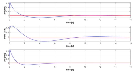
Figure 4. Euler angles signals [$\mathsf{\varphi }\left(\mathsf{t}\right), \mathsf{\vartheta }\left(\mathsf{t}\right),\mathsf{\psi }\left(\mathsf{t}\right)$] of the controlled attitude system (blue): PID-based Attitude Stabilizer (red).

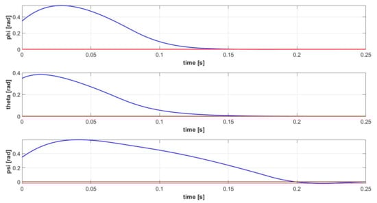
Figure 5. Euler angles signals [$\mathsf{\varphi }\left(\mathsf{t}\right), \mathsf{\vartheta }\left(\mathsf{t}\right),\mathsf{\psi }\left(\mathsf{t}\right)]$ of the controlled attitude system (blue): LQR-based Attitude Stabilizer (red).

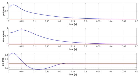
Figure 6. Euler angles signals [$\mathsf{\varphi }\left(\mathsf{t}\right), \mathsf{\vartheta }\left(\mathsf{t}\right),\mathsf{\psi }\left(\mathsf{t}\right)$] of the controlled attitude system (blue): FL-based Attitude Stabilizer (red).

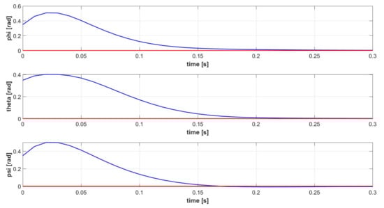
Figure 7. Euler angles signals [$\mathsf{\varphi }\left(\mathsf{t}\right), \mathsf{\vartheta }\left(\mathsf{t}\right),\mathsf{\psi }\left(\mathsf{t}\right)$] of the controlled attitude system (blue): SMC-based Attitude Stabilizer (red).

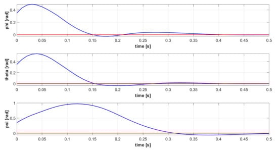
Figure 8. Euler angles signals [$\mathsf{\varphi }\left(\mathsf{t}\right), \mathsf{\vartheta }\left(\mathsf{t}\right),\mathsf{\psi }\left(\mathsf{t}\right)$] of the controlled attitude system (blue): MPC-based Attitude Stabilizer (red).

The three pairs of proportional, integral and derivative gains of the PID-based attitude controller are tuned exploiting the automatic tuning library in MATLAB applied to the linearized system in (26), considering the control input saturation, to achieve a fast (rise time of ~1 s) and robust step response. As shown in Figure 4, the Euler angles dynamics relative to the PID-based stabilizer are much slower with respect to all the others, meaning that PID control is effective but requires extensive gain tuning and is not robust to model uncertainties, as the performances significantly decrease when the controller is applied to the nonlinear attitude system. As far as the classical PID control approach is concerned, which is the approach adopted in this work, a systematic procedure exists for tuning the controller’s gains; however, a highly time-consuming offline gains optimization is required when dealing with nonlinear systems, as for quadrotor UAVs. The amount of computation related to the online optimization of the MPC-based attitude stabilizer is such that the optimal solution is computed, on average, within 0.01 s. A control horizon ${\mathrm{T}}_{\mathrm{z}}=0.05\mathrm{s}$ is chosen in order to guarantee the optimal controller command at each step. A trial-and-error tuning procedure is adopted for the choice of the control parameters of the other attitude stabilizers, which show faster dynamics and greater robustness to model uncertainties. The sum of the L₂ norms of the Euler angles’ tracking error signals, L₂^x, is chosen as the approximative evaluation parameter of the controllers’ tracking performance. Analogously, the sum of the L₂ norms of the controller command signals, L₂^u, represents the approximative evaluation parameter of the expected command activity of an on-board hardware implementation of the controller. Since the L₂ norm of a signal represents the “energy” associated with the signal itself, it can be considered as an approximative quantitative estimation of both the overall tracking error and the controller command effort. Table 3 shows the controllers’ evaluation parameters referring to the attitude stabilization simulations presented in this section.

Table 3. Evaluation parameters: sum of L₂ norms of the controller commands signals, L₂^u, and sum of L₂ norms of the Euler angles error signals, L₂^x.

Attitude Stabilizer.	L2u	L2x
PID	1.60	1.40
LQR	4.53	0.41
FL	5.6	0.64
SMC	4.35	0.36
MPC	3.70	0.65

The proposed attitude stabilizers are ranked from best to worse as SMC, LQR, FL, MPC, PID for L₂^x and as PID, MPC, SMC, LQR, FL for L₂^u. Considering the attitude controllers that lead to the fastest dynamics (SMC, LQR and FL), the choice of the inner loop control law derives from a trade-off between tracking performances and controller command effort, since the battery consumption, being related to the forces and moments required to act on the quadcopter platform, is a key limitation factor when dealing with multirotor UAVs executing medium-to-long range missions. The SMC-based attitude stabilizer is the most promising one, having minimum L₂^x, intermediate L₂^u and ensuring fast dynamics to the controlled variables. Besides the norm evaluation, the FL-based controller yields to bigger peaks in the controlled signals. It is worth noting that ad-hoc simulation campaigns may be designed in order to tune the control parameters of each attitude stabilizer such that the system achieves a reference dynamic response. This could enhance performance, but the inherent features of each control approach would not change, as well as the highlighted differences among the methods.

3.2. Closed-Loop System

The complete controlled quadrotor system is proven to be able to execute complex 3D trajectories, defined by Equations (62)–(64). Both an ascent helix (trajectory 1) and a more complex ascent helix (trajectory 2) are simulated. The signals related to the controlled variables are shown in Figure 9 for trajectory 1, Figure 10 shows the corresponding quadcopter’s 3D trajectory, Figure 11 shows the control command signals required for executing trajectory 1. The Euler Angles signals related to trajectory 1 are shown in Figure 12. The signals related to the controlled variables are shown in Figure 13 for trajectory 2, Figure 14 shows the corresponding quadcopter’s 3D trajectory, Figure 15 shows the control command signals required for executing trajectory 2. The Euler Angles signals related to trajectory 2 are shown in Figure 16. Considering that either PID control is a model-free approach with an easy gain tuning procedure, or the outer loop controller is intended to ensure a much slower dynamic response with respect to the inner loop controller (order of a few seconds), a PID controller in the outer loop is sufficient to ensure a satisfactory dynamic response. The tracking performances are satisfactory for either the sinusoidal-based or the unitary step reference velocity signals, as shown in Figure 9 and Figure 13, which spatially derive in the helicoidal maneuvers shown in Figure 10 and Figure 14. Due to the inherent characteristics of PID control, a relatively small delay between the sinusoidal-based reference velocity signal and the actual quadcopter velocity is inevitable. That is reflected also in a smaller, yet present, delay in the tracking of the consequent sinusoidal-based Euler angles signals, as shown in Figure 12 and Figure 16. Overall, the proposed architecture can effectively control the quadcopter during complex maneuvers without exceeding the saturation limits, as shown by the signals of the controller commands in Figure 11 and Figure 15.

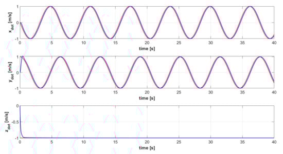
Figure 9. Velocity signals [${\mathrm{X}}^{\prime }\left(\mathsf{t}\right),{ \mathrm{Y}}^{\prime }\left(\mathsf{t}\right),{ \mathrm{Z}}^{\prime }\left(\mathsf{t}\right)$] of the controlled quadrotor system (blue) and reference velocity signals of trajectory 1 (red).

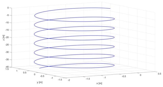
Figure 10. 3D view of trajectory 1: position trajectory of the controlled quadrotor system.

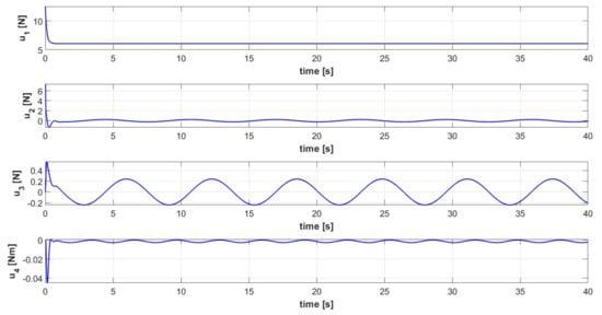
Figure 11. Control input signals [${\mathrm{u}}_1\left(\mathsf{t}\right),{ \mathrm{u}}_2\left(\mathsf{t}\right),{ \mathrm{u}}_3\left(\mathsf{t}\right),{ \mathrm{u}}_4\left(\mathsf{t}\right)$] of the controlled quadrotor system executing trajectory 1.

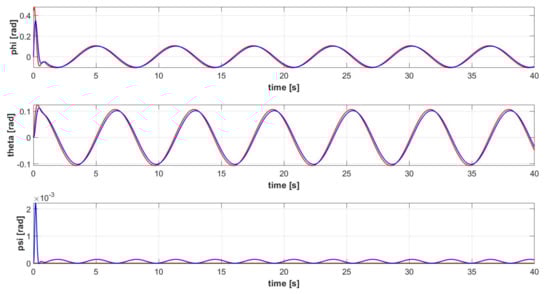
Figure 12. Euler angles signals [$\mathsf{\varphi }\left(\mathsf{t}\right), \mathsf{\vartheta }\left(\mathsf{t}\right),\mathsf{\psi }\left(\mathsf{t}\right)$] of the controlled quadrotor system (blue) and reference attitude signals for trajectory 1 (red).

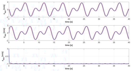
Figure 13. Velocity signals [$X^{\prime }\left(\mathsf{t}\right),{ \mathrm{Y}}^{\prime }\left(\mathsf{t}\right),{ \mathrm{Z}}^{\prime }\left(\mathsf{t}\right)$] of the controlled quadrotor system (blue) and reference velocity signals of trajectory 2 (red).

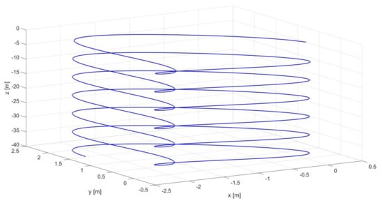
Figure 14. 3D view of trajectory 2: position trajectory of the controlled quadrotor system.

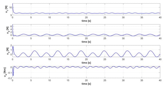
Figure 15. Control input signals [${\mathrm{u}}_1\left(\mathsf{t}\right),{ \mathrm{u}}_2\left(\mathsf{t}\right),{ \mathrm{u}}_3\left(\mathsf{t}\right),{ \mathrm{u}}_4\left(\mathsf{t}\right)$] of the controlled quadrotor system executing trajectory 2.

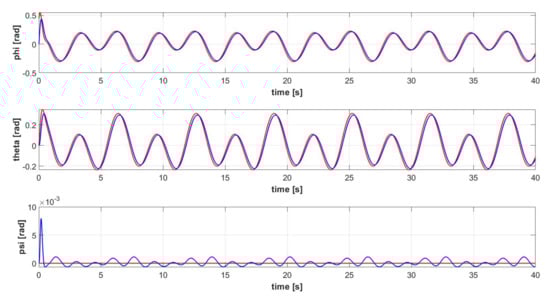
Figure 16. Euler angles signals [$\mathsf{\varphi }\left(\mathsf{t}\right), \mathsf{\vartheta }\left(\mathsf{t}\right),\mathsf{\psi }\left(\mathsf{t}\right)$] of the controlled quadrotor system (blue) and reference attitude signals for trajectory 2 (red).

4. Conclusions

In this paper, a control system architecture for 3D trajectory tracking is implemented and simulated in MATLAB/Simulink^® for a micro-quadrotor UAV. The highly nonlinear, coupled, unstable and underactuated plant system, i.e., the quadrotor, is modelled with the Newton–Euler formalism. The control architecture is intended to stabilize the quadrotor attitude dynamics, which is fully actuated with a sufficiently fast inner loop controller, and to track velocity references in the outer loop. A comparative study of well-known linear and nonlinear model-free and model-based control laws applied to the attitude stabilization problem is proposed: PID, LQR, FL, SMC and MPC attitude stabilization laws are designed and implemented. The choice of the inner loop controller derives from either the fast dynamics requirement of the inner loop or an L₂ norm-based approximative evaluation of both tracking error and controller command signals since the relatively poor battery autonomy is still one of the main limitations for the deployment of multirotor UAVs in medium-to-long range missions. The reference attitude signals for the inner loop controller are derived from a simplified translational dynamics inversion performed in an outer loop controller, which is also responsible for altitude control. In the outer loop, the dynamics inversion is combined with three independent PID controllers, while the Sliding Mode attitude stabilizer is implemented in the inner loop. A velocity trajectory generator and a control input saturation block complete the proposed control architecture. The controlled closed-loop quadrotor system is proven to be able to execute complex 3D trajectories, such as ascent helixes. Consistent with the aim of this work, the main summarizing considerations are reported in Table 4 in order to highlight the main observations drawn from the study and provide guidelines for further research in this field.

Table 4. Summarizing table of considerations drawn from the study. The number of diamonds is proportional to the “suitability of the method to UAV control”.

Control Method	Advantages	Disadvantages	Overall Suitability to UAV Control
PID	Systematic gain tuning method for linear systems Possible zero steady state error Model free	No constraints handling Poor robustness No multiple inputs and multiple outputs handling Extensive offline gain optimization	◊
LQR	Possible handling of multiple inputs and multiple outputs Possible handling of performance and command effort Fast dynamics	May fail to overcome steady-state error	◊◊◊
FL	Systematic cancellation of nonlinearities	No constraints handling Poor robustness Model in affine form only	◊◊
SMC	Robustness Fast dynamics Good performances with highly nonlinear systems	Chattering may cause instability	◊◊◊◊
MPC	Possible handling of multiple inputs and multiple outputs Possible handling of performance and command effort Possible handling of input and output constraints	Slow dynamics	◊◊

Future research directions will include the realization of other comparative studies for control of quadrotor UAVs, considering external disturbances, e.g., the wind, and parametric uncertainties, e.g., variable payloads.

References

- Cohen, A.; Shaheen, A.; Farrar, E. Urban Air Mobility: History, Ecosystem, Market Potential, and Challenges. IEEE Trans. Intell. Transp. Syst. 2022, 22, 6074–6087. [Google Scholar] [CrossRef]
- Nawaz, H.; Ali, H.M.; Massan, S.U.R. Applications of unmanned aerial vehicles: A review. 3c Tecnol. Glosas Innovación Apl. Pyme. 2019, 2019, 85–105. [Google Scholar]
- Aslan, M.F.; Durdu, A.; Sabanci, K.; Ropelewska, E.; Gültekin, S.S. A Comprehensive Survey of the Recent Studies with UAV for Precision Agriculture in Open Fields and Greenhouses. Appl. Sci. 2022, 12, 1047. [Google Scholar] [CrossRef]
- Skrinjar, J.P.; Skorput, P.; Furdic, M. Application of Unmanned Aerial Vehicles in Logistic Processes. In Proceedings of the New Technologies, Development and Applications (NT-2018), Sarajevo, Bosnia and Herzegovina, 14–16 June 2018. [Google Scholar]
- Idrissi, M.; Salami, M.R.; Annaz, F. A Review of Quadrotor Unmanned Aerial Vehicles: Applications, Architectural Design and Control Algorithms. J. Intell. Robot. Syst. 2022, 104, 22. [Google Scholar]
- Roy, R.; Islam, M.; Sadman, N.; Mahmud, M.A.P.; Gupta, K.D.; Ahsan, M.M. A Review on Comparative Remarks, Performance Evaluation and Improvement Strategies of Quadrotor Controllers. Technologies 2021, 9, 37. [Google Scholar]
- Shauqee, M.N.; Rajendran, P.; Suhadis, N.M. Quadrotor Controller Design Techniques and Applications Review. Incas Bull. 2021, 13, 179–194. [Google Scholar]
- Zulu, A.; John, S. A Review of Control Algorithms for Autonomous Quadrotors. Open J. Appl. Sci. 2014, 4, 547–556. [Google Scholar] [CrossRef]
- Shraim, H.; Awada, A.; Youness, R. A survey on quadrotors: Configurations, modeling and identification, control, collision avoidance, fault diagnosis and tolerant control. IEEE Aerosp. Electron. Syst. Mag. 2018, 33, 14–33. [Google Scholar] [CrossRef]
- Bolandi, H.; Rezaei, M.R.; Mohsenipour, R.; Nemati, H.; Smailzadeh, S.M. Attitude Control of a Quadrotor with Optimized PID Controller. Intell. Control Autom. 2013, 4, 335–342. [Google Scholar] [CrossRef]
- Voos, H. Nonlinear control of a quadrotor micro-UAV using feedback-linearization. In Proceedings of the 2009 IEEE International Conference on Mechatronics, Malaga, Spain, 14–17 April 2009. [Google Scholar]
- Islam, M.; Okasha, M.; Idres, M. Dynamics and Control of Quadcopter using Linear Model Predictive Control Approach. In Proceedings of the AEROS Conference 2017, Putrajaya, Malaysia, 12 December 2017. [Google Scholar]
- Madani, T.; Benallegue, A. Backstepping Control for a Quadrotor Helicopter. In Proceedings of the 2006 IEEE/RSJ International Conference on Intelligent Robots and Systems, Beijing, China, 9–15 October 2006. [Google Scholar]
- Petrusevski, I.; Aleksandar, R. Simple fuzzy solution for quadrotor attitude control. In Proceedings of the 12th Symposium on Neural Network Applications in Electrical Engineering (NEUREL), Belgrade, Serbia, 25–27 November 2014. [Google Scholar]
- Capello, E.; Guglieri, G.; Quagliotti, F.; Sartori, D. Design and Validation of an L1 Adaptive Controller for Mini-UAV Autopilot. J. Intell. Robot. Syst. 2013, 69, 109–118. [Google Scholar] [CrossRef]
- Noordin, A.; Mohd Basri, M.A.; Mohamed, Z. Position and Attitude Tracking of MAV Quadrotor Using SMC-Based Adaptive PID Controller. Drones 2022, 6, 263. [Google Scholar] [CrossRef]
- Sankaranarayanan, V.N.; Satpute, S.; Nikolakopoulos, G. Adaptive Robust Control for Quadrotors with Unknown Time-Varying Delays and Uncertainties in Dynamics. Drones 2022, 6, 220. [Google Scholar] [CrossRef]
- Shakeel, T.; Arshad, J.; Jaffery, M.H.; Rehman, A.U.; Eldin, E.T.; Ghamry, N.A.; Shafiq, M. A Comparative Study of Control Methods for X3D Quadrotor Feedback Trajectory Control. Appl. Sci. 2022, 12, 9254. [Google Scholar] [CrossRef]
- Okasha, M.; Kralev, J.; Islam, M. Design and Experimental Comparison of PID, LQR and MPC Stabilizing Controllers for Parrot Mambo Mini-Drone. Aerospace 2022, 9, 298. [Google Scholar] [CrossRef]
- Available online: https://basecamp-shop.com/en/product/dji-quadcopter-flame-wheel-arf-kit-450 (accessed on 18 November 2022).
- Ghazbi, S.N.; Aghli, Y.; Alimohammadi, M.; Akbari, A.A. Quadrotors Unmanned Aerial Vehicles: A Review. Int. J. Smart Sens. Intell. Syst. 2016, 9, 309–333. [Google Scholar] [CrossRef]
- Zhang, X.; Li, X.; Wang, K.; Lu, Y. A Survey of Modelling and Identification of Quadrotor Robot. Abstr. Appl. Anal. 2014, 2014, 1–16. [Google Scholar] [CrossRef]
- Moness, M.; Bakr, M. Development and Analysis of Linear Model Representations of the Quad-Rotor System. In Proceedings of the Aerospace Sciences and Aviation Technology, Cairo, Egypt, 26–28 May 2015. [Google Scholar]
- Naidoo, Y.; Stopforth, R.; Bright, G. Quad-Rotor Unmanned Aerial Vehicle Helicopter Modelling & Control. Int. J. Adv. Robot. Syst. 2011, 8, 139–149. [Google Scholar]
- Astrom, K.J.; Hagglund, T. Advanced PID Control; Instrumentation, Systems and Automation Society: Pittsburgh, PA, USA, 2006. [Google Scholar]
- Dorato, P.; Abdallah, C.; Cerone, V. Linear Quadratic Control: An Introduction; Krieger Pub Co.: Malabar, FL, USA, 2000. [Google Scholar]
- Krener, A.J. Feedback Linearization. In Mathematical Control Theory; Baillieul, J., Willems, J.C., Eds.; Springer: New York, NY, USA, 1999; pp. 66–98. [Google Scholar]
- Edwards, C.; Spurgeon, S. Sliding Mode Control: Theory and Applications; CRC Press: London, UK, 1998. [Google Scholar]
- Yan, B.; Dai, P.; Liu, R.; Xing, M.; Liu, S. Adaptive super-twisting sliding mode control of variable sweep morphing aircraft. Aerosp. Sci. Technol. 2019, 92, 198–210. [Google Scholar] [CrossRef]
- Rawlings, J.B.; Mayne, D.Q.; Diehl, M.M. Model Predictive Control: Theory, Computation, and Design; Nob Hill Publishing: Santa Barbara, CA, USA, 2020. [Google Scholar]
Disclaimer/Publisher’s Note: The statements, opinions and data contained in all publications are solely those of the individual author(s) and contributor(s) and not of MDPI and/or the editor(s). MDPI and/or the editor(s) disclaim responsibility for any injury to people or property resulting from any ideas, methods, instructions or products referred to in the content. |
© 2023 by the authors. Licensee MDPI, Basel, Switzerland. This article is an open access article distributed under the terms and conditions of the Creative Commons Attribution (CC BY) license (https://creativecommons.org/licenses/by/4.0/).