A New Approach to Nonlinear State Observation for Affine Control Dynamical Systems

Abstract

In this work, a Nonlinear Higher Order Extended State Observer (NHOESO) is presented to replace the Linear Extended State Observer (LESO) used in Conventional Active Disturbance Rejection Control (C-ADRC) solutions. In the NHOESO, the standard LESO is completed with a two-term smooth nonlinear function with saturation-like characteristics. The proposed novel NHOESO enables precise observation of the generalized disturbances with higher-order derivatives. The stability of the NHOESO is examined with the aid of the Lyapunov method. A simulation of an uncertain nonlinear Single-Input–Single-Output (SISO) system with time-varying external disturbances confirms that the proposed NHOESO copes well with the generalized disturbance, which is not true for other ESOs.

1. Introduction

Observers gather increasing amounts of information about the states of systems from their inputs and outputs [1,2,3,4,5,6]. The first state observation was made by Luenberger [7] by observing inputs and outputs, and numerous subsequent versions, including sliding-mode observers [8] and high-gain observers [9], have been proposed since. Unlike its predecessors, the Extended State Observer (ESO) was pioneering in its independence from mathematical models [10]. Active Disturbance Rejection Control (ADRC) was used to estimate the uninformative dynamics of a nonlinear system as well as the model uncertainties that contribute to the generalized disturbance [11]. As reported in [10], ADRC was proposed to address the shortcomings of PID controllers. Several versions of ADRC were based on a nonlinear version of the ESO [12] and were parameterized in [13]. The main components of ADRC are a Tracking Differentiator (TD), a Nonlinear State Error Feedback (NLSEF), and an Extended State Observer (ESO) [14,15,16].

1.1. Related Works

In [17], an Unknown Input Observer (UIO) was proposed and used for Disturbance Accommodation Control (DAC). The external disturbance is considered an extra-state variable of the plant model. The UIO estimates the entire state, and the disturbance is cancelled with a specifically selected counteracting control signal. A Disturbance Observer (DOB) was designed in [18]. It uses the inverse of the nominal transfer function of the plant and rejects exogenous disturbances. Based on the concept of the DOB, a Multi-loop Perturbation Compensator (MPEC) was proposed in [19]. A hierarchical and recursive compensation method effectively compensates the perturbation (i.e., model uncertainty and external disturbances) to the plant. There was great improvement in the perturbation attenuation performance as the number of loops increased, but there was a reduction in the robust stability margin on the modeling error as the loop number increased. As explained in [20], the UIO offered superior application value compared to the DOB because provided an estimation of the state variables and did not only estimate the disturbance. A Nonlinear Disturbance Observer (NDO) was proposed in [21]. Such an NDO has been used in robotic manipulator systems, such as planar serial manipulators with revolute joints [22], and multi-fingered robot hands [23].

In [24], an extended high-gain observer for nonlinear MIMO systems, in which the observer dynamics are faster than the extended system dynamics, was proposed by feeding back the output estimation error via a nonlinear function, and the nonlinear ESO (NLESO) was designed. There are two types of nonlinear functions: those that fit the rule of “big error, small gain”, and those that fit the rule of “small error, big gain” [25]. the nonlinear function is generally chosen as a piecewise continuous, saturating, monotonically increasing function [26,27,28]. The nonlinear gains of the NLESO are designed to reduce the “peaking phenomenon” and to avoid large transient behaviors [29]. A nonlinear observer was also used to guarantee fast convergence and robustness concerning noise [30]. In [31,32], a generic NLESO has been given. In [33,34], two different nonlinear functions have been proposed. These nonlinear functions have not only a nonlinear characteristic but also have better smoothness properties. In particular, these functions can be separately adjusted to be suited to the practical application with different requirements through three design parameters. A function with two design parameters that change the shape and range of the function was proposed in [35]. A non-smooth function, which is a combination of linear and nonlinear terms, has been proposed in [25,26,28,36,37,38] with two design parameters. Unfortunately, using this function has introduced a high-frequency chattering phenomenon [33,35]. The work in [39] selected the hyperbolic tangent function without any parameter to ensure rapid convergence. In [40], the output estimation error was fed back using both nonlinear and switching terms to establish a novel finite-time convergent ESO. The motion control of a speed turntable with a temperature box was applied with the proposed ESO. This ESO performed better than a traditional ESO based on the experimental results. In [41], an ESO with time-varying gain was introduced to reduce drastically the peaking value. A detailed analysis with rigorous mathematical proof for the NLESO, which is the backbone of ADRC, was given in [32]. In [42], an ESO with high-order nonlinearity was studied using the Describing Function (DF) method. In addition, the nonlinear ESO and ADRC parameters were tuned using a simple and fast method.

1.2. Paper Contribution

The NHOESO proposed in this paper is based on the conventional ESO and includes a two-term smooth nonlinear function with saturation-like properties. The proposed NHOESO will make it possible to observe the generalized disturbances with high accuracy. The experiment in [4] demonstrated that the nonlinear function $fal\left(e,\alpha ,\delta \right)$, suggested as

$$fal\left(e,\alpha ,\delta \right)=\left\{\begin{array}{c}\begin{array}{cc}\frac{e}{{\delta }^{1-\alpha }}\hfill & \left|e\right|\le \delta \hfill \end{array}\hfill \\ \begin{array}{cc}{\left|e\right|}^{\alpha }sgn\left(e\right)\hfill & \left|e\right|>\delta \hfill \end{array}\hfill \end{array}\right.$$

(1)

is rough, and whatever the value of $\delta$ is, the phenomenon of high-frequency chattering is still present. Thus, the main contributions of this paper are as follows:

• A new class of nonlinear function $𝒢\left(e\right): ℝ\to ℝ$ proposed as

  $$𝒢\left(e\right)=K_{\alpha }{\left|e\right|}^{\alpha }sign\left(e\right)+K_{\beta }{\left|e\right|}^{\beta }e$$

  is used instead of the $fal\left(e,\alpha ,\delta \right)$ function. This nonlinear function has a nonlinear characteristic and is smooth;
• Moreover, the curve shape, range, and central location of this function can be separately adjusted to adapt to the practical application of different situations and requirements;
• The saturation-like properties are used to suggest a novel asymptotically convergent extended state observer. The proposed NHOESO can enhance the observation capability and asymptotically reduce the estimation error when compared to traditional extended state observers;
• Additionally, a precise Lyapunov analysis of the NHOESO and the associated closed-loop system was performed. The NHOESO-based controller can sustain zero tracking error and is asymptotically stable.

To the best of our knowledge, no NHOESO for extremely uncertain nonlinear systems has yet been proposed in the literature. This problem is significant and difficult for reasons related to theory and practice, which is our incentive for continuing this research endeavor.

1.3. Paper Organization

This paper is outlined as follows. In Section 2, the statement of the underlying problem is discussed. A LESO and its parameter tuning method are introduced in Section 3. Section 4 presents the suggested NHOESO, which is the contribution of this work. An analysis of the validity of the observer proposed in Section 5 is based on numerical simulations. Lastly, Section 6 provides the conclusion.

2. Problem Statement

Given a $n\mathrm{th}$ order nonlinear system of relative degree $\rho$, with $\rho \le n$,

$$\left\{\begin{array}{c}{\xi }^{\left(\rho \right)}=f\left(\xi ,\dots ,{\xi }^{\left(\rho -1\right)},\eta ,w,t\right)+b\left(t\right)u\left(t\right)\hfill \\ \begin{array}{c}y=\xi \hfill \\ \dot{\eta }=f_0\left(\eta ,\xi ,\dots ,{\xi }^{\left(\rho -1\right)}\right)\hfill \end{array}\hfill \end{array}\right.$$

(2)

where $\xi$ is the system’s states, $u\left(t\right)\in \mathrm{C}\left(ℝ,ℝ\right)$ is the control input, $y\left(t\right)\in \mathrm{C}\left(ℝ, ℝ\right)$ is the measured output, $w\left(t\right)\in \mathrm{C}\left(ℝ, ℝ\right)$ is an external disturbance,$b\left(t\right)\in \mathrm{C}\left(ℝ, ℝ\right)$ is the input gain, and $f_0\in \mathrm{C}\left({ℝ}^n,{ℝ}^{n-\rho }\right)$ is the nonlinear function that represents the internal dynamics. $f\in \mathrm{C}\left({ℝ}^{\rho }\times ℝ\times ℝ\times ℝ,ℝ\right)$ is an unknown uncertain function. It should be noted that System (2) is not in the “pure chain of integrators” form or what is called the Brunovsky form.

If the ESO is incorporated into the feedback loop, it will guarantee that (2) will be put into the Brunovsky form up to $\rho$. Through the ADRC, the generalized disturbance from the nonlinear system in (2) is removed online using the estimated states $\hat{\xi }$. As in [43], consider the following assumptions for System (2).

Assumption A1.

There is information available about the input and output signals of the system and its relative degree.

3. Linear Extended State Observer (LESO)

Assume ${\xi }_1=y,{\xi }_2=\dot{y},\dots ,{\xi }_{\rho }={\xi }^{\left(\rho -1\right)}$, then,

$$\left\{\begin{array}{c}{\dot{\xi }}_i={\xi }_{i+1} i\in \left\{1,2,\dots ,\rho -1\right\}\hfill \\ {\dot{\xi }}_{\rho }=f\left({\xi }_1,{\xi }_2,\dots ,{\xi }_{\rho },w,t\right)+\left(b\left(t\right)-b_0\right)u+b_{0}u\hfill \end{array}\right.$$

(3)

Consider the additional state,

$${\xi }_{\rho +1}=f+\left(b\left(t\right)-b_0\right)u=L$$

(4)

where $L$ is denoted as the generalized disturbance, which comprises all unidentified external disturbances, internal dynamics, and uncertainties. Several methods are used to choose the value of the parameter $b_0\in ℝ\backslash \left\{0\right\}$. In [10], the coefficient $b_0$ is a loose estimation of $b\left(t\right)$ in the range of ±50%, while in [43], the parameter $b_0$ was chosen empirically by the user as a design parameter.

Assumption A2.

There exists an upper bound for the time derivative of the generalized disturbance (i.e., at least $L\in C^1$ and $su{p}_{t\in \left[0,\infty \right)}\left|L\right|=M<\infty$ where $\in ℝ$).

Based on Assumptions A1 and A2, a ${\left(\rho +1\right)}^{th}$ order LESO can be designed to estimate both the generalized disturbances and the states of the system given in (2) following the method presented by [44],

$$\left\{\begin{array}{c}{\dot{\hat{\xi }}}_i={\hat{\xi }}_{i+1}+{\beta }_i\left(y-{\hat{\xi }}_1\right), i\in \left\{1,2,\dots ,\rho -1\right\}\hfill \\ {\dot{\hat{\xi }}}_{\rho }={\hat{\xi }}_{\rho +1}+{\beta }_{\rho }\left(y-{\hat{\xi }}_1\right)+b_{0}u\hfill \\ {\dot{\hat{\xi }}}_{\rho +1}={\beta }_{\rho +1}\left(y-{\hat{\xi }}_1\right)\hfill \end{array}\right.$$

(5)

where ${\beta }_i$ is an observer gain coefficient to be adjusted and $i=1,2,\dots ,\rho +1$, $\left(y-{\hat{\xi }}_1\right)=e$ is the estimation error. The bandwidth-based and pole placement methods are the traditional techniques to adjust a linear extended state observer. If the aim is to lower the number of coefficients, the observer gain parameters may be expressed as functions of the bandwidth ${\omega }_0$ of the LESO. The estimator gains are chosen as

$$\left(\begin{array}{c}{\beta }_1\\ {\beta }_2\\ \begin{array}{c}⋮\\ {\beta }_{\rho +1}\end{array}\end{array}\right)=\left(\begin{array}{c}{a}_1{\omega }_0\\ a_2{\omega }_0^2\\ \begin{array}{c}⋮\\ a_{\rho +1}{\omega }_0^{\rho +1}\end{array}\end{array}\right)$$

where $a_i,i=1,2,\dots ,\rho +1$ are selected in such a way that the characteristics equation $s^{\rho +1}+a_1{s}^{\rho }+\dots +a_{\rho }s+a_{\rho +1}$ is stable Hurwitz. Large values of the LESO parameters will increase the adverse effect of the measurement noise, and thus will decrease the system performance. Moreover, large values of the LESO parameters lead to the “peaking phenomenon”, which is caused by multiplying the estimation error $e=(y-{\hat{\xi }}_1$) by large values. Therefore, there is a need to adopt a new class of ESO that relieves the effect of the aforementioned issues. Nonlinear ESO is a new class of ESO that manipulates the estimation error $e=(y-{\hat{\xi }}_1$) in a nonlinear fashion and can alleviate the effect of both measurement noise and the peaking phenomenon.

4. The Proposed Nonlinear Higher-Order Extended State Observer (NHOESO)

4.1. The NHOESO Definition and Convergence Theorem

To extend the concept of the linear extended state observer (LESO), two major improvements are included in this work. Firstly, a smooth nonlinear error function is introduced. Secondly, adding more than one augmented state to the proposed NHOESO enables it to track the generalized disturbance ${\xi }_{\rho +1}$ asymptotically. Moreover, the estimation error $e_i\left(t\right), i\in \left\{1,2,\dots ,\rho \right\}$ depends on the upper bound of the second derivative of the generalized disturbance ${\xi }_{\rho +1}$. This aspect allows the NHOESO to estimate disturbances and uncertainties with higher-order derivatives. As was shown in the simulation, these improvements provided faster and more accurate estimations of the states ${\xi }_i, i\in \left\{1,2,\dots ,\rho \right\}$ and the generalized disturbance ${\xi }_{\rho +1}$. The proposed nonlinear error function also reduced the chattering phenomenon presented in LESOs. In addition, the proposed NHOESO produced both a smooth control signal and a minimum overshoot in the output response.

Starting from the nonlinear system of (3) and adding the extended states ${\xi }_{\rho +1}=f+\left(b\left(x\right)-b_0\right)u=L$, ${\xi }_{\rho +2}=\dot{L}$, System (3) can be written equivalently as

$$\left\{\begin{array}{c}{\dot{\xi }}_i={\xi }_{i+1}, i\in \left\{1,2,\dots ,\rho -1\right\}\hfill \\ {\dot{\xi }}_{\rho }={\xi }_{\rho +1}+b_{0}u\hfill \\ \begin{array}{c}{\dot{\xi }}_{\rho +1}={\xi }_{\rho +2}\hfill \\ {\dot{\xi }}_{\rho +2}={\Delta }_h\hfill \end{array}\hfill \end{array}\right.$$

(6)

where ${\Delta }_h\left(t\right)=\ddot{L}.$

The proposed NHOESO is described as

$$\left\{\begin{array}{c}{\dot{\hat{\xi }}}_i={\hat{\xi }}_{i+1}+{\beta }_i𝒢\left(e\right), i\in \left\{1,2,\dots ,\rho -1\right\}\hfill \\ {\dot{\hat{\xi }}}_{\rho }={\hat{\xi }}_{\rho +1}+{\beta }_{\rho }𝒢\left(e\right)+b_{0}u\hfill \\ \begin{array}{c}{\dot{\hat{\xi }}}_{\rho +1}={\hat{\xi }}_{\rho +2}+{\beta }_{\rho +1}𝒢\left(e\right)\hfill \\ {\dot{\hat{\xi }}}_{\rho +2}={\beta }_{\rho +2}𝒢\left(e\right)\hfill \end{array}\hfill \end{array}\right.$$

(7)

where $e=(y-{\hat{\xi }}_1$) is the estimation error and the parameters ${\beta }_i$,$i=\left\{1,2,\dots ,\rho +2\right\}$ are the gains of the estimator to be adjusted. It is supposed that ${\beta }_i=a_i{\omega }_0{}^i$, where $a_i$, $i\in \left\{1,2,\dots ,\rho +2\right\}$ is the related design parameter with each ${\omega }_0{}^i$, and ${\omega }_0$ is the bandwidth of the NHOESO estimator.

The function $𝒢:ℝ\to ℝ$ is proposed as

$$𝒢\left(e\right)=K_{\alpha }{\left|e\right|}^{\alpha }sign\left(e\right)+K_{\beta }{\left|e\right|}^{\beta }e$$

(8)

where $e=(y-{\hat{\xi }}_1$) is the estimation error, $K_{\alpha },K_{\beta },\alpha , and \beta$ are positive design parameters, i.e., $\alpha , \beta >0$. The suggested function $𝒢\left(e\right)$ of (8) can be expressed as

$$𝒢\left(e\right)=\left(K_{\alpha }\frac{{\left|e\right|}^{\alpha }}{e}sign\left(e\right)+K_{\beta }{\left|e\right|}^{\beta }\right)e$$

(9)

Since sign ($e$) = $e$/|$e$|, for $\left|e\right|\ne 0$, then

$$𝒢\left(e\right)=\left\{\begin{array}{c}\begin{array}{cc}0 \hfill & e=0\hfill \end{array}\hfill \\ \begin{array}{cc}k\left(e\right)e \hfill & e\ne 0\hfill \end{array}\hfill \end{array}\right.$$

(10)

Function $k\left(e\right):ℝ/\left\{0\right\}\to {ℝ}^{+}$ is an even function, given as

$$k\left(e\right)=K_{\alpha }{\left|e\right|}^{\alpha -1}+K_{\beta }{\left|e\right|}^{\beta }$$

(11)

To prove the convergence of the NHOESO, the following assumptions are needed:

Assumption A3.

L is a continuously differentiable function.

Assumption A4.

There exists $M_h\in {ℝ}^{+}$ such that$su{p}_{t\in \left[0,\infty \right)}\left|{\Delta }_h\left(t\right)\right|=M_h$, where  ${\Delta }_h\left(t\right)=\ddot{L}$.

Assumption A5.

$V:{ℝ}^{\rho +2}\to {ℝ}^{+}$ and $W:{ℝ}^{\rho +2}\to {ℝ}^{+}$ are continuously differentiable functions with

$${\lambda }_1{\Vert \eta \Vert }^2\le V\left(\eta \right)\le {\lambda }_2{\Vert \eta \Vert }^2, W\left(\eta \right)={\Vert \eta \Vert }^2$$

(12)

$${{\displaystyle \sum }}_{i=1}^{\rho +1}\frac{\partial V\left(\eta \right)}{{\eta }_i}\left({\eta }_{i+1}-a_{i}k\left(\frac{{\eta }_1}{{\omega }_0{}^{\rho }}\right)·{\eta }_1\right)-\frac{\partial V\left(\eta \right)}{\partial y_{\rho +2}}{a}_{\rho +2}k\left(\frac{{\eta }_1}{{\omega }_0{}^{\rho }}\right){\eta }_1\le -W\left(\eta \right)$$

(13)

Theorem 1. (NHOESO convergence):

Given System (6) and NHOESO (7), it follows that, under Assumptions A3, A4, and A5, for any initial conditions,

$$\underset{t\to \infty }{\mathit{lim}}\left|{\xi }_i\left(t\right)-{\hat{\xi }}_i\left(t\right)\right|=O\left(\frac{1}{{\omega }_0{}^{\rho +3-i}}\right)$$

$$\underset{\begin{array}{c}t\to \infty \hfill \\ {\omega }_0\to \infty \hfill \end{array}}{\mathit{lim}}\left|{\xi }_i\left(t\right)-{\hat{\xi }}_i\left(t\right)\right|=0$$

where ${\xi }_i$ and ${\hat{\xi }}_i$ symbolize the states of (6) and (7) respectively, with $i\in \left\{1,2,\dots ,\rho +2\right\}$.

Proof: see Appendix A.

4.2. Justification for Adding an Additional Augmented State

The reason to incorporate more additional states in the proposed NHOESO is explained in this subsection. The analysis of the steady-state estimation error $e_i\left(t\right), i\in \left\{1,2,\dots ,\rho +1\right\}$ of the LESO can be found in [11],

$$\underset{t\to \infty }{\mathit{lim}}\left|{\xi }_i-{\hat{\xi }}_i\right|=\frac{1}{{\omega }_0{}^{\rho +2-i}}\frac{2M{\lambda }^2{}_{max}\left(P\right)}{{\lambda }_{min}\left(P\right)}$$

(14)

while that of the NHOESO is found in Theorem 1,

$$\underset{t\to \infty }{\mathit{lim}}\left|{\xi }_i-{\hat{\xi }}_i\right|=\frac{1}{{\omega }_0{}^{\rho +3-i}}\frac{2M_h{\lambda }^2{}_{max}\left(P\right)}{{\lambda }_{min}\left(P\right)}$$

(15)

These results illustrate that the steady-state estimation error $\underset{t\to \infty }{\mathit{lim}}\left|{\xi }_i-{\hat{\xi }}_i\right|$ of the NHOESO is more sensitive to an increase in the bandwidth ${\mathsf{\omega }}_0$ than that of the LESO. This is because of the presence of ${\mathsf{\omega }}_0$ in the denominator. Moreover, the steady-state estimation errors are proportional to $M$ for the LESO as in (14) and to $M_h$ for the NHOESO as in (15), where $M_h$ and $M$ are the limit bounds of the second and first derivatives of the generalized disturbance ${\xi }_{\rho +1},$ respectively (see Assumptions A2 and A4)

Consider a generalized disturbance ${\xi }_{\rho +1}$, which is a linear function in time, i.e., $L\left(t\right)=at$, where $\mathrm{a}$ is a constant. Then $\Delta =\dot{L}=a$ and ${\Delta }_h=\ddot{L}=0$, and based on this, the upper bound $M$, is a non-zero constant, while ${\mathrm{M}}_{\mathrm{h}}$ is zero. In this case, for a specific low value of ${\omega }_0$, the steady-state estimation error of the NHOESO in (15) will be zero, while that of the LESO given in (14) has a non-negligible value. Therefore, the NHOESO is more suitable than the LESO to give an estimation of the generalized disturbance ${\xi }_{\rho +1}$ of the linear type. Moreover, a generalized disturbance ${\xi }_{\rho +1}$ with a higher-order derivative will worsen the steady-state estimation error for the LESO because if the generalized disturbance ${\mathsf{\xi }}_{\mathsf{\rho }+1}$ is expressed as $L\left(t\right)=a{t}^2$, then the upper bound $M\to \infty$, as $t\to \infty$. The steady-state estimation error of the LESO will escape to infinity, i.e., $\underset{t\to \infty }{\mathit{lim}}\left|{\xi }_i-{\hat{\xi }}_i\right|\to$ $\infty$, and thus, the LESO will diverge. However, $M_h$ will have a constant value of $2\mathrm{a}$. Consequently, the NHOESO will have a small steady-state estimation error for sufficiently large NHOESO bandwidth ${\omega }_0$. The only weak point of the NHOESO is the time required for the estimated generalized disturbance ${\hat{\xi }}_3$ to be settled to its actual value ${\xi }_3$, which is analyzed in the following example.

Consider a situation where the relative degree $\rho =2$, and the LESO is expressed as

$$\left\{\begin{array}{c}{\dot{\hat{\xi }}}_1={\hat{\xi }}_2+{\beta }_1\left(y-{\hat{\xi }}_1\right),\hfill \\ {\dot{\hat{\xi }}}_2={\hat{\xi }}_3+{\beta }_2\left(y-{\hat{\xi }}_1\right)+b_{0}u, \hfill \\ {\dot{\hat{\xi }}}_3={\beta }_3\left(y-{\hat{\xi }}_1\right)\hfill \end{array}\right.$$

(16)

The dynamics of the NHOESO given in (7) with $𝒢\left(y-{\hat{\xi }}_1\right)=y-{\hat{\xi }}_1$ is expressed as

$$\left\{\begin{array}{c}{\dot{\hat{\xi }}}_1={\hat{\xi }}_2+{\beta }_1\left(y-{\hat{\xi }}_1\right),\hfill \\ {\dot{\hat{\xi }}}_2={\hat{\xi }}_3+{\beta }_2\left(y-{\hat{\xi }}_1\right)+b_{0}u,\hfill \\ \begin{array}{c}{\dot{\hat{\xi }}}_3={\hat{\xi }}_4+{\beta }_3\left(y-{\hat{\xi }}_1\right),\hfill \\ {\dot{\hat{\xi }}}_4={\beta }_4\left(y-{\xi }_1\right)\hfill \end{array}\hfill \end{array}\right.$$

(17)

Given that ${\hat{\xi }}_4=\int {\beta }_4\left(y-{\xi }_1\right) dt$, then (17) can be expressed as

$$\left\{\begin{array}{c}{\dot{\hat{\xi }}}_1={\hat{\xi }}_2+{\beta }_1\left(y-{\hat{\xi }}_1\right),\hfill \\ {\dot{\hat{\xi }}}_2={\hat{\xi }}_3+{\beta }_2\left(y-{\hat{\xi }}_1\right)+b_{0}u,\hfill \\ {\dot{\hat{\xi }}}_3={\beta }_4{{\displaystyle \int }}_0^t\left(y-{\hat{\xi }}_1\right) dt+{\beta }_3\left(y-{\hat{\xi }}_1\right)\hfill \end{array}\right.$$

(18)

It is shown in Theorem 1 that $\underset{t\to \infty }{\mathit{lim}}\left|{\xi }_1-{\hat{\xi }}_1\right|=\frac{1}{{\omega }_0{}^{\rho +2}}\frac{2M_h{\lambda }^2{}_{max}\left(P\right)}{{\lambda }_{min}\left(P\right)}$, where the R.H.S is a constant ($\rho$, ${\omega }_0$, ${\lambda }_{min}\left(P\right)$, ${\lambda }_{max}\left(P\right)$, $\mathrm{and}{M}_h$ are constants). So, given that $y={\xi }_1$ and if Equation (23) has integration term ${\beta }_4{{\displaystyle \int }}_0^t\left(y-{\hat{\xi }}_1\right)dt$, then, the result of the integration will be constant too. It can be noticed in (16) that the estimated generalized disturbance ${\hat{\xi }}_3$ is a function of the error $e_1=y-{\hat{\xi }}_1$ and will change in accordance with the error. It will settle to its actual value ${\xi }_3$ when the estimation error $y-{\hat{\xi }}_1$ becomes zero. Meanwhile, in the NHOESO (18), and due to the integration term ${\beta }_4{{\displaystyle \int }}_0^t\left(y-{\hat{\xi }}_1\right)dt$, the estimated generalized disturbance ${\hat{\xi }}_3$ of the NHOESO will take a longer time to settle to its actual value ${\xi }_3$, which requires the following condition:

$${\beta }_4{{\displaystyle \int }}_0^t\left(y-{\hat{\xi }}_1\right) dt+{\beta }_3\left(y-{\hat{\xi }}_1\right)=0$$

(19)

Letting $e_1=y-{\hat{\xi }}_1$, (19) can be expressed as

$${\beta }_4{{\displaystyle \int }}_0^t{e}_1 dt+{\beta }_3{e}_1=0$$

(20)

Taking the derivative of (20) w.r.t $t$, we obtain

$${\dot{e}}_1=-\frac{{\beta }_4}{{\beta }_3}{e}_1$$

(21)

Solving (21) w.r.t $t$, yields

$$e_1\left(t\right)=e_1\left(0\right)exp\left(-\frac{{\beta }_4}{{\beta }_3}t\right)$$

Therefore, the condition (19) will be satisfied at $t\to \infty$ (i.e., $t=-\frac{{\beta }_3}{{\beta }_4}ln\left(\frac{e_1\left(t\right)}{e_1\left(0\right)}\right)$ when $e_1\left(t\right)$ has a very small value), or as the ratio $\frac{{\beta }_4}{{\beta }_3}$ is large enough, where $e_1\left(t\right)=e_1\left(0\right)exp\left(-\frac{{\beta }_4}{{\beta }_3}t\right)$ will decay faster to zero.

4.3. Mismatched Disturbances

To satisfy the matched condition, the ESO assumes that the plant is expressed in the normal form [45,46]. Thus, it can only be applied to systems that can be expressed in the normal form directly or by changing variables. When a system has zero dynamics, performing such a transformation can be challenging. There are also nonlinear systems with disturbances appearing in a different channel of control input, and these systems fail to satisfy the matching condition. Due to this, the ADRC is no longer able to manipulate this mismatched disturbance as before. For instance, the following nonlinear model belongs to a class of uncertain nonlinear systems in a lower triangular form with mismatched disturbance [47,48,49,50,51,52]:

$$\left\{\begin{array}{c}{\xi }_i=a_i{\xi }_{i+1}+{\varphi }_i\left({\xi }_1,\dots ,{\xi }_i\right)+w_i, i\in \left\{1,2,\dots ,\rho -1\right\}\hfill \\ {\xi }_{\rho }={\varphi }_{\rho }\left({\xi }_1,{\xi }_2,\dots ,{\xi }_{\rho }\right)+w_{\rho }+bu,\hfill \\ y={\xi }_1.\hfill \end{array}\right.$$

(22)

where $\xi ={\left({\xi }_1\left(t\right),{\xi }_2\left(t\right),\dots ,{\xi }_{\rho }\left(t\right)\right)}^T\in {ℝ}^{\rho }$ is the system state, $y\left(t\right)\in ℝ$ is the measured output, $u\left(t\right)\in ℝ$ is the control input,$w_i\left(t\right)\in ℝ, i\in \left\{1,2,\dots ,\rho \right\}$ is the unknown exogenous disturbance, and $b\in ℝ$ is the control coefficient. The function ${\varphi }_i:{ℝ}^i\to ℝ, i\in \left\{1,2,\dots ,\rho \right\}$.

Theorem 2.

A second-order nonlinear system in a lower triangular form with mismatched disturbances can be described as follows:

$$\left\{\begin{array}{c}{\dot{\xi }}_1=a_1{\xi }_2+{\varphi }_1\left({\xi }_1\right)+w_1\hfill \\ {\dot{\xi }}_2={\varphi }_2\left({\xi }_1,{\xi }_2\right)+w_2+bu\hfill \\ y={\xi }_1\hfill \end{array}\right.$$

(23)

where $\xi ={\left({\xi }_1\left(t\right),{\xi }_2\left(t\right)\right)}^T\in {ℝ}^2$ is the system’s state, $y\left(t\right)\in ℝ$ is the measured output, $u\left(t\right)\in ℝ$ is the control input, $w_i\left(t\right)\in ℝ, i\in \left\{1,2\right\}$ is the unknown exogenous disturbance, and $b\in ℝ$ is the control coefficient. The function ${\varphi }_i:{ℝ}^i\to ℝ, i\in \left\{1,2\right\}$. If the function ${\varphi }_1$ and the exogenous disturbance $w_1$ are differentiable w.r.t $t$, System (23) can be transformed into the following form:

$$\left\{\begin{array}{c}{\dot{\tilde{\xi }}}_1={\tilde{\xi }}_2,\hfill \\ {\dot{\tilde{\xi }}}_2=f\left({\tilde{\xi }}_1,{\tilde{\xi }}_2,w_1,{\dot{w}}_1,w_2\right)+\hat{b}u,\hfill \\ y={\tilde{\xi }}_1.\hfill \end{array}\right.$$

(24)

where $f\left({\tilde{\xi }}_1,{\tilde{\xi }}_2,w_1,{\dot{w}}_1,w_2\right)=a_1{\varphi }_2\left({\tilde{\xi }}_1,\frac{{\tilde{\xi }}_2-{\varphi }_1\left({\tilde{\xi }}_1\right)-w_1}{a_1}\right)+\frac{\partial {\varphi }_1\left({\tilde{\xi }}_1\right)}{\partial {\xi }_1}{\tilde{\xi }}_2+a_1{w}_2+{\dot{w}}_1$ and $\hat{b}=a_{1}b$.

Proof: seen Appendix A.

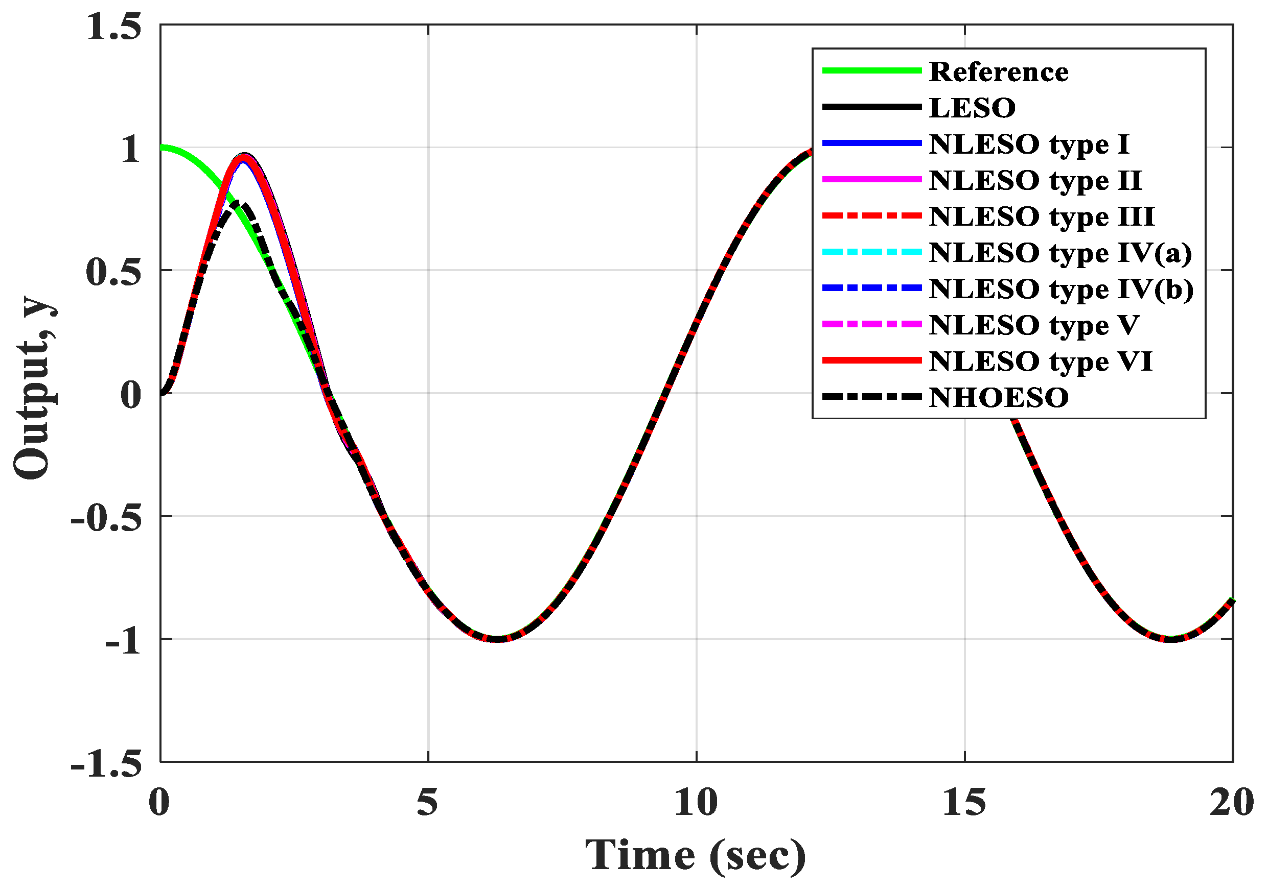
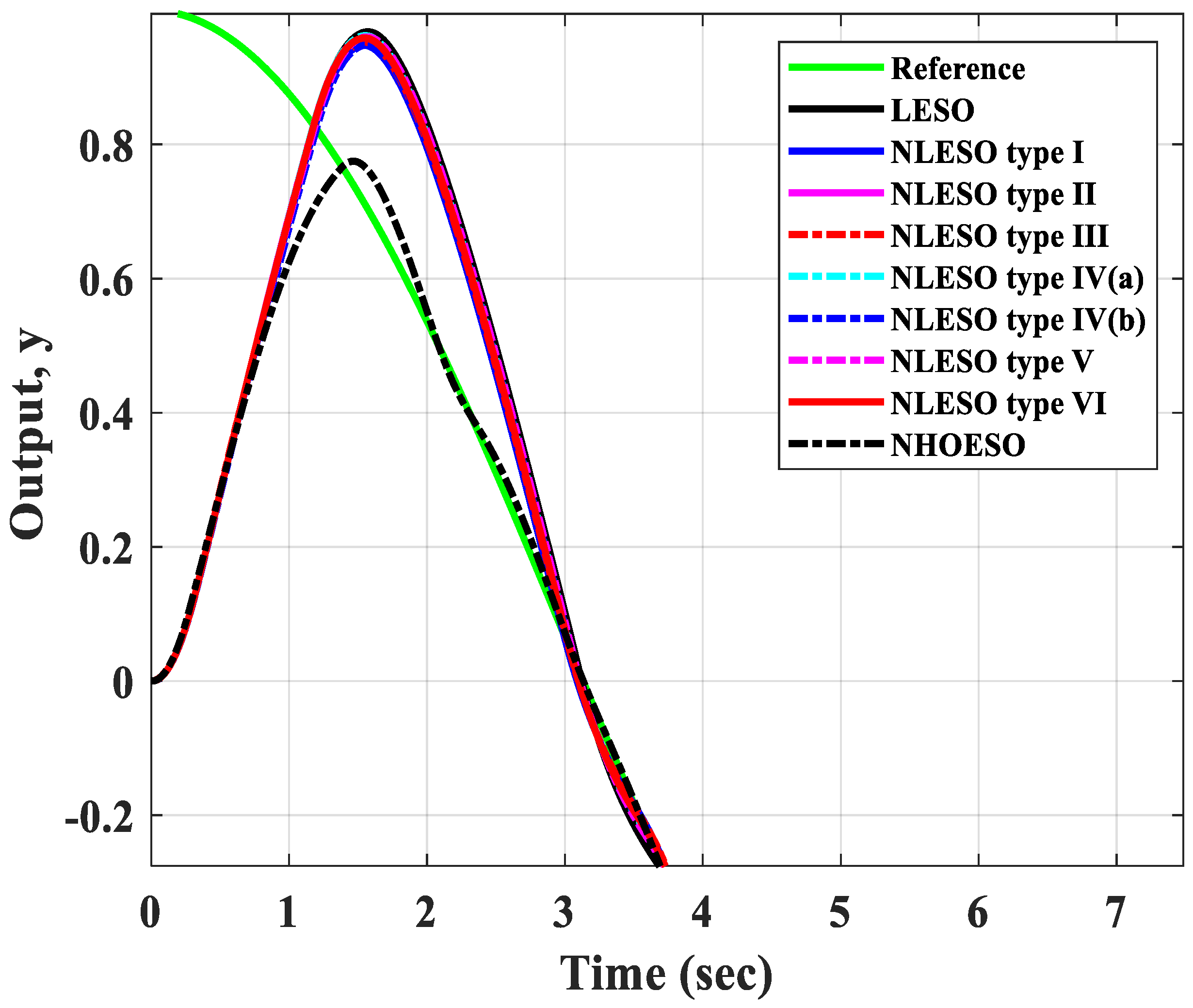
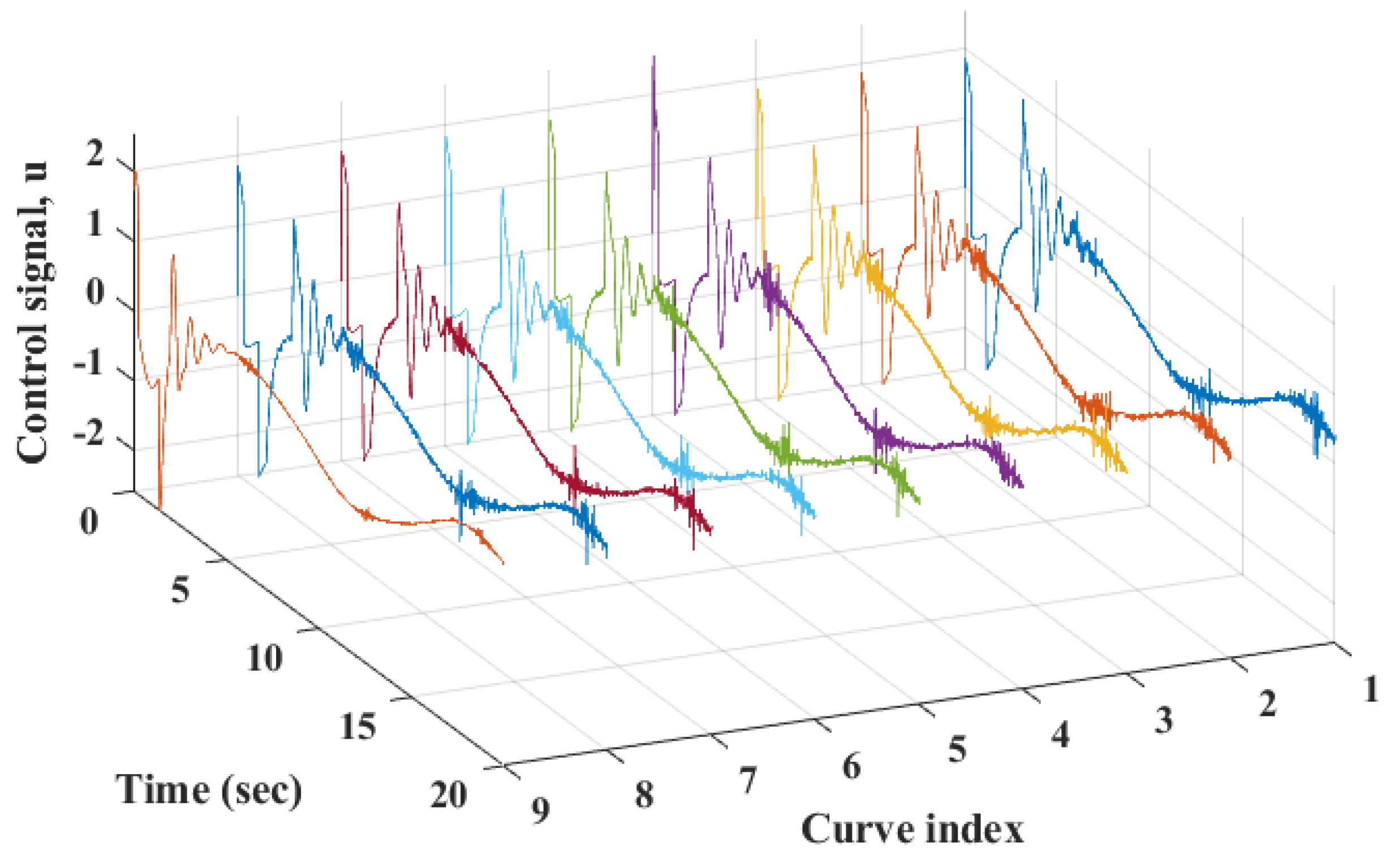
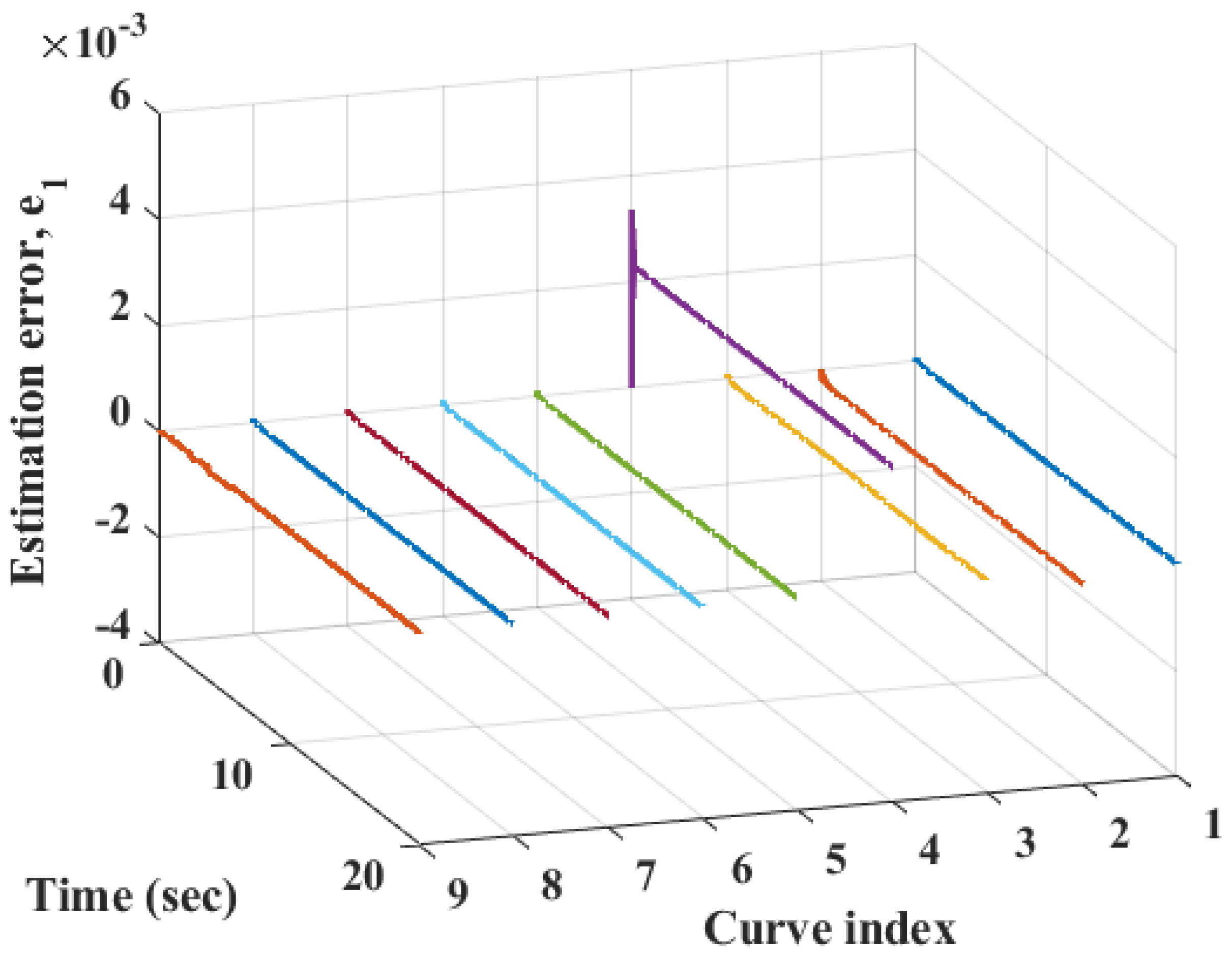
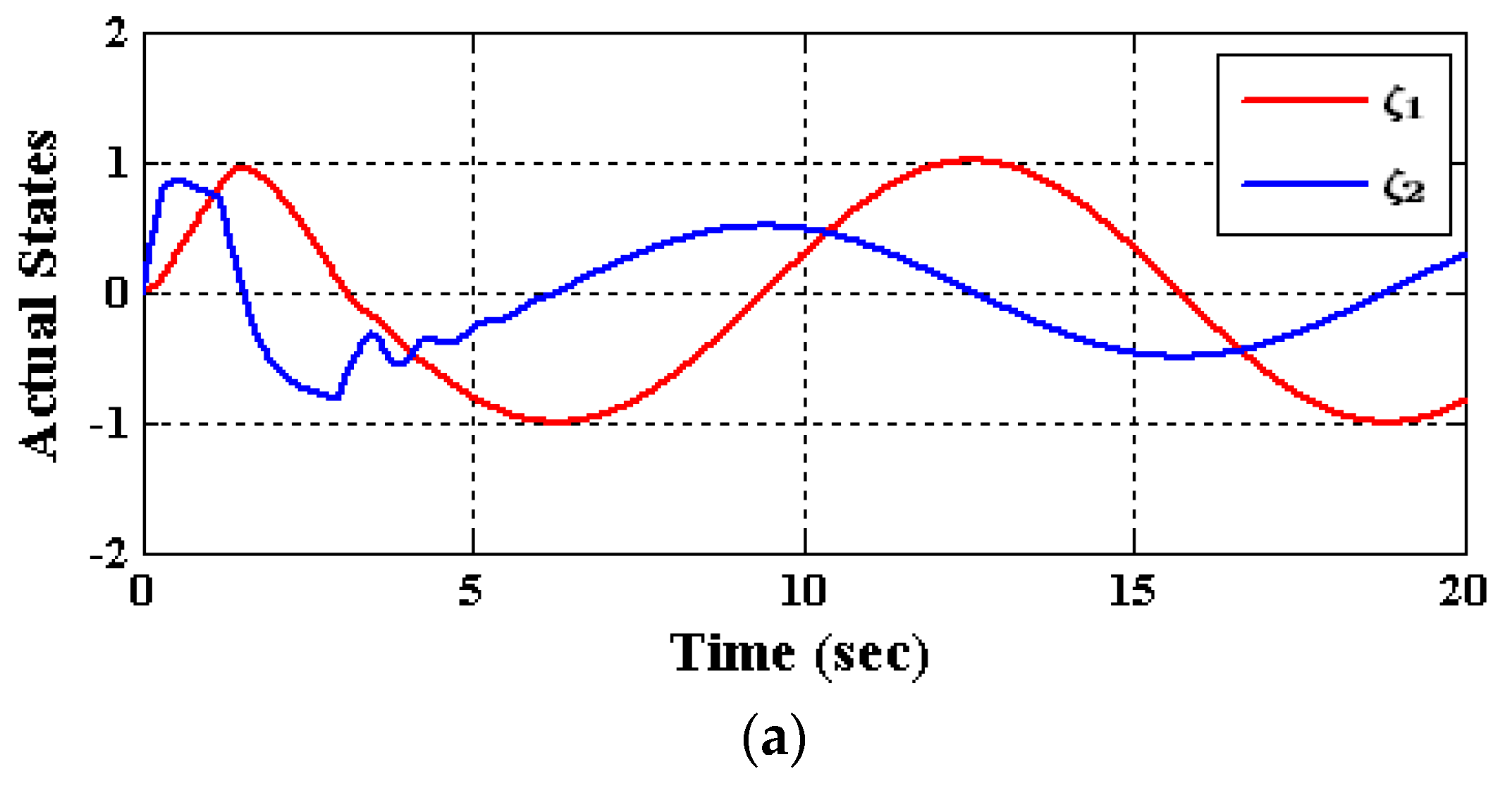
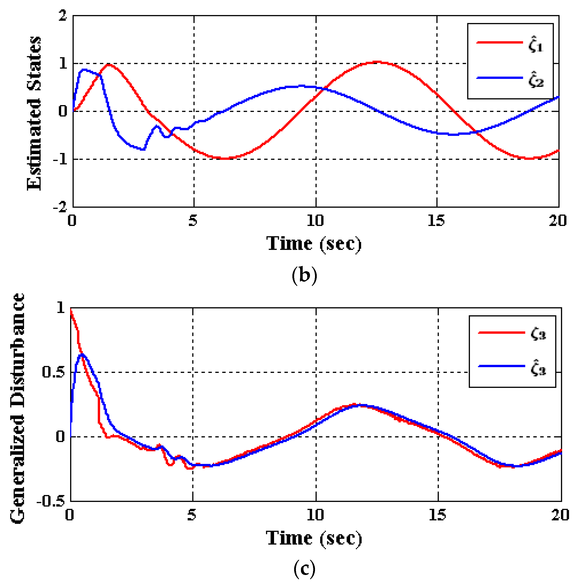
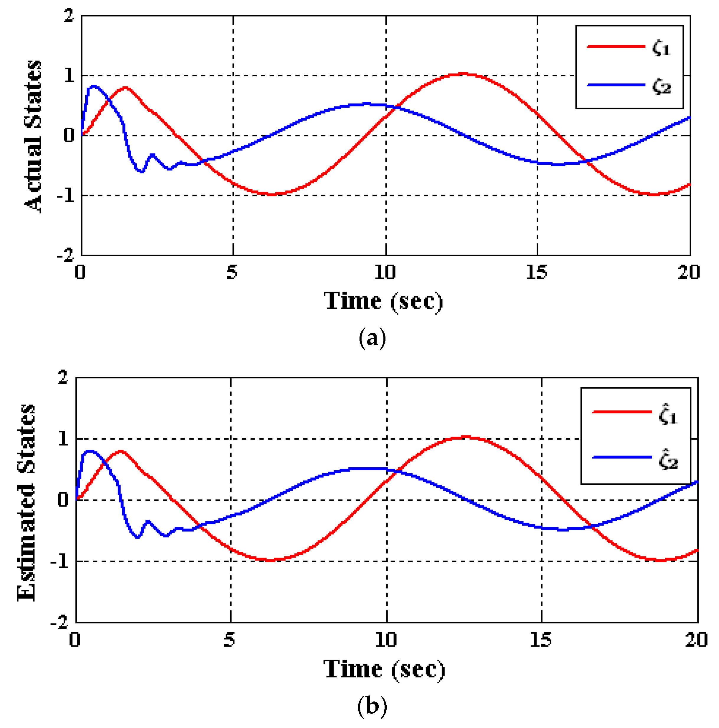
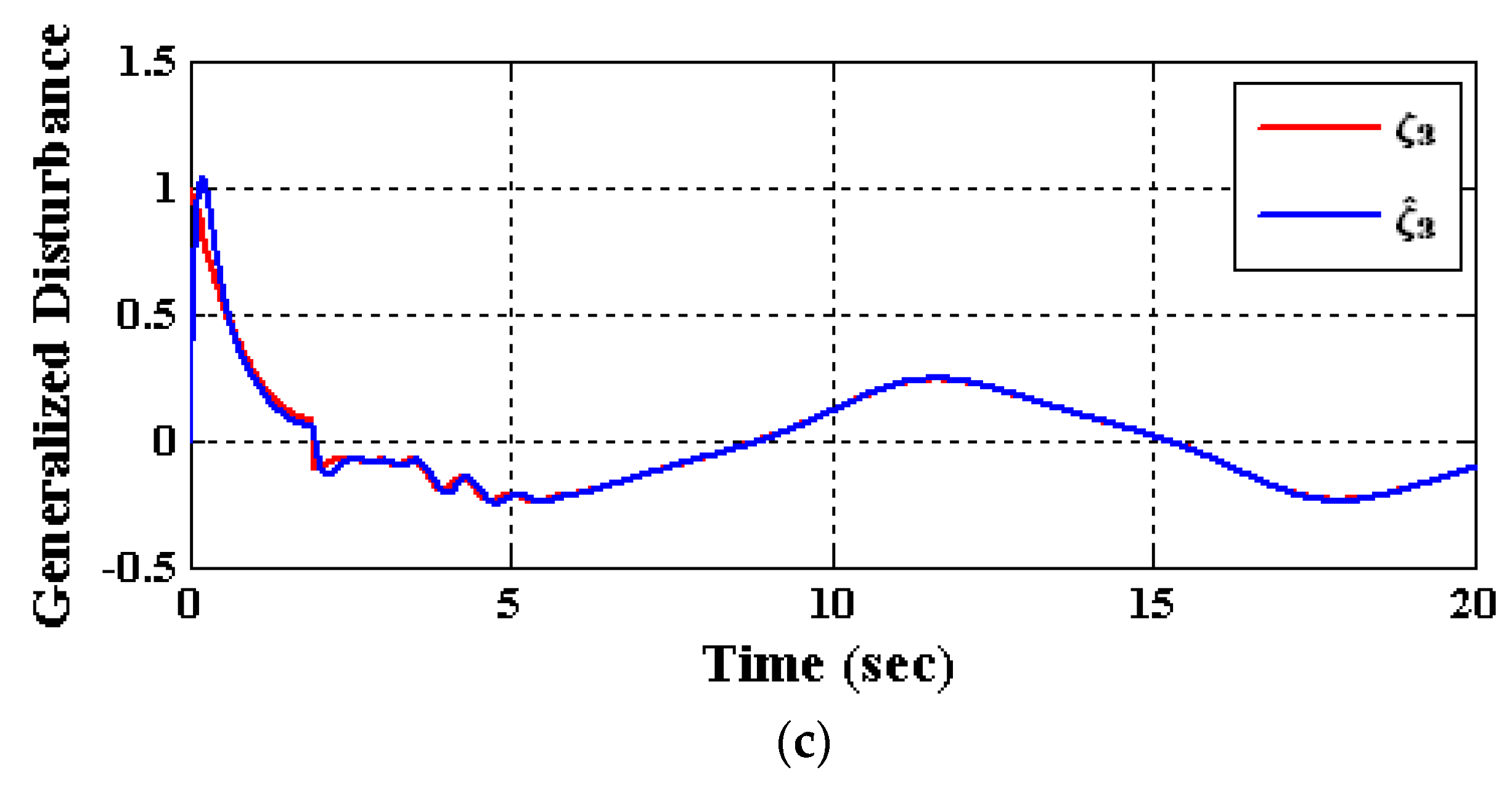
5. Numerical Simulations

To assess the effectiveness of the suggested NHOESO, the following nonlinear SISO system is considered:

$$\left\{\begin{array}{c}{\dot{\xi }}_1={\xi }_2\hfill \\ \begin{array}{c}{\dot{\xi }}_2=f\left({\xi }_1,{\xi }_2\right)+w\left(t\right)+\left(1+{\mathrm{a}}_3\sin \left(t\right)\right)u\hfill \\ y=x_1\hfill \end{array}\hfill \end{array}\right.$$

(25)

where $f\left({\xi }_1,{\xi }_2\right)=a_1{\xi }_1+a_{2}sin\left({\xi }_2\right)$, with $a_1=0.2$, $a_2=a_3=0.1$, and the external disturbances are taken as $w\left(t\right)=\exp \left(-t\right)\cos \left(t\right)$. The reference $r\left(t\right)$ was selected as a periodic input and was defined as $\cos \left(0.5t\right)$ imposed at t = 0 s.

The fall-based control law in this simulation is

$$u=fal\left({\tilde{e}}_1,{\alpha }_1,{\delta }_1\right)+fal\left({\tilde{e}}_2,{\alpha }_2,{\delta }_2\right)-{\hat{\xi }}_3$$

(26)

where

$$fal\left(e,\alpha ,\delta \right)=\left\{\begin{array}{c}\begin{array}{cc}\frac{e}{{\delta }^{1-\alpha }} \hfill & \left|e\right|\le \delta \hfill \end{array}\hfill \\ \begin{array}{cc}{\left|e\right|}^{\alpha }sgn\left(e\right)\hfill & \left|e\right|>\delta \hfill \end{array}\hfill \end{array}\right.$$

The error of the tracking is steering the control signal given by ${\left({\tilde{e}}_1, {\tilde{e}}_2\right)}^T={\left(r_1, r_2\right)}^T-{\left({\hat{\xi }}_1, {\hat{\xi }}_2\right)}^T$. The desired transient profile vector ${\left(r_1, r_2\right)}^T$ is obtained using a conventional Tracking Differentiator (TD), given as [10]:

$$\left\{\begin{array}{c}{\dot{r}}_1=r_2,\hfill \\ {\dot{r}}_2=-Rsign\left(r_1-r+\frac{r_2\left|r_2\right|}{2R}\right)\hfill \end{array}\right.$$

(27)

Different ESOs have been chosen from the literature to be compared with our proposed NHOESO. They were used to find the estimated states ${\left({\hat{\xi }}_1,{\hat{\xi }}_2\right)}^T$ and the estimated generalized disturbance ${\hat{\xi }}_3$. The combination of the conventional TD of (34), the fall-based control law of (26), and the proposed NHOESO of (7) is called NHOESO-based ADRC (written as NADRC in the following). The dynamics of the observers that were used in these simulations are listed in

Table 1. The list of the ESOs used in the comparison.

Index	The Type of ESO	Dynamics
1	LESO [44]	${\dot{\hat{\xi }}}_1={\hat{\xi }}_2+{\beta }_1\left(y-{\hat{\xi }}_1\right)$ ${\dot{\hat{\xi }}}_2={\hat{\xi }}_3+{\beta }_2\left(y-{\hat{\xi }}_1\right)$         ${\dot{\hat{\xi }}}_3={\beta }_3\left(y-{\hat{\xi }}_1\right)$
2	NLESO type I [33]	${\dot{\hat{\xi }}}_1={\hat{\xi }}_2+{\beta }_1{f}_1\left(y-{\hat{\xi }}_1\right)$ ${\dot{\hat{\xi }}}_2={\hat{\xi }}_3+{\beta }_2{f}_1\left(y-{\hat{\xi }}_1\right)$ ${\dot{\hat{\xi }}}_3={\beta }_3{f}_1\left(y-{\hat{\xi }}_1\right)$    where $f_1\left(e\right)=\frac{b_{1}tan\left(b_2\left(e-b_3\right)-\tan \left(-b_2{b}_3\right)\right)}{\frac{\pi }{2}-tan\tan \left(-b_2{b}_3\right)}$
3	NLESO type II [35]	${\dot{\hat{\xi }}}_1={\hat{\xi }}_2+{\beta }_1{f}_2\left(y-{\hat{\xi }}_1\right)$ ${\dot{\hat{\xi }}}_2={\hat{\xi }}_3+{\beta }_2{f}_2\left(y-{\hat{\xi }}_1\right)$ ${\dot{\hat{\xi }}}_3={\beta }_3{f}_2\left(y-{\hat{\xi }}_1\right)$    where $f_2\left(e\right)=b_1\left(1-e^{b_{2}e}\right)sign\left(e\right)$
4	NLESO type III [34]	${\dot{\hat{\xi }}}_1={\hat{\xi }}_2+{\beta }_1{f}_3\left(y-{\hat{\xi }}_1\right)$ ${\dot{\hat{\xi }}}_2={\hat{\xi }}_3+{\beta }_2{f}_3\left(y-{\hat{\xi }}_1\right)$ ${\dot{\hat{\xi }}}_3={\beta }_3{f}_3\left(y-{\hat{\xi }}_1\right)$    where $f_3\left(e\right)=b_1(\frac{\pi }{4}-arc\tan (b_2{e}^{-b_2\left(e-b_3\right)}$)
5	NLESO type IV(a) [53]	${\dot{\hat{\xi }}}_1={\hat{\hat{\xi }}}_2+{\beta }_{1}fal\left(y-{\hat{\hat{\xi }}}_1,\alpha ,\delta \right)$ ${\dot{\hat{\xi }}}_2={\hat{\hat{\xi }}}_3+{\beta }_{2}fal\left(y-{\hat{\hat{\xi }}}_1,\alpha ,\delta \right)$       ${\dot{\hat{\xi }}}_3={\beta }_{3}fal\left(y-{\hat{\hat{\xi }}}_1,\alpha ,\delta \right)$
6	NLESO type IV(b) [25]	${\dot{\hat{\xi }}}_1={\hat{x}}_2+{\beta }_{1}fal\left(y-{\hat{\hat{\xi }}}_1,{\alpha }_1,{\delta }_1\right)$ ${\dot{\hat{\xi }}}_2={\hat{\hat{\xi }}}_3+{\beta }_{2}fal\left(y-{\hat{\hat{\xi }}}_1,{\alpha }_2,{\delta }_2\right)$       ${\dot{\hat{\xi }}}_3={\beta }_{3}fal\left(y-{\hat{\hat{\xi }}}_1,{\alpha }_3,{\delta }_3\right)$
7	NLESO type V [39]	${\dot{\hat{\xi }}}_1={\hat{\hat{\xi }}}_2+{\beta }_{1}tanh\left(y-{\hat{\hat{\xi }}}_1\right)$ ${\dot{\hat{\xi }}}_2={\hat{\hat{\xi }}}_3+{\beta }_{2}tanh\left(y-{\hat{\hat{\xi }}}_1\right)$       ${\dot{\hat{\xi }}}_3={\beta }_{3}ftanh\left(y-{\hat{\hat{\xi }}}_1\right)$
8	NLESO type VI [29]	${\dot{\hat{\xi }}}_1={\hat{\hat{\xi }}}_2+{\beta }_{1}fal\left(y-{\hat{\hat{\xi }}}_1,\alpha ,\delta \right)+k_1\left(y-{\hat{\hat{\xi }}}_1\right)$ ${\dot{\hat{\xi }}}_2={\hat{\hat{\xi }}}_3+{\beta }_{2}fal\left(y-{\hat{\hat{\xi }}}_1,\alpha ,\delta \right)+k_2\left(y-{\hat{\hat{\xi }}}_1\right)$     ${\dot{\hat{\xi }}}_3={\beta }_{3}fal\left(y-{\hat{\hat{\xi }}}_1,\alpha ,\delta \right)+k_3\left(y-{\hat{\hat{\xi }}}_1\right)$
9	Proposed NHOESO	${\dot{\hat{\xi }}}_1={\hat{\hat{\xi }}}_2+{\beta }_1𝒢\left(y-{\hat{\hat{\xi }}}_1\right)$ ${\dot{\hat{\xi }}}_2={\hat{\hat{\xi }}}_3+{\beta }_2𝒢\left(y-{\hat{\hat{\xi }}}_1\right)$ ${\dot{\hat{\xi }}}_3={\hat{\hat{\xi }}}_4+{\beta }_3𝒢\left(y-{\hat{\hat{\xi }}}_1\right)$ ${\dot{\hat{\xi }}}_4={\beta }_4𝒢\left(y-{\hat{\hat{\xi }}}_1\right)$    where $𝒢\left(e\right)=k_{\alpha }{\left|e\right|}^{\alpha }sign\left(e\right)+k_{\beta }{\left|e\right|}^{\beta }e$

. The time responses of these simulations are shown in Figure 1, Figure 2, Figure 3 and Figure 4. In this work, an OPI is proposed, which is represented as

$$OPI=w_1\frac{ITAE}{N_1}+w_2\frac{ISU}{N_2}+$$

(28)

where $\mathrm{ITAE}={{\displaystyle \int }}_0^{t_f}t\left|y-r\right|dt$ is the integration of the time absolute error for the output signal, $\mathrm{ISU}={{\displaystyle \int }}_0^{t_f}{v}^2 dt$ is the integration of the square of the control signal, $\mathrm{IAU}={{\displaystyle \int }}_0^{t_f}\left|v\right|dt$ is the integration of the absolute of the control signal, and $t_f$ is the final simulation time. The tuning process of the ADRC units and the conventional techniques was carried out using the Genetic Algorithm (GA) in the MATLAB^® environment to minimize the OPI of (28). The sample data of the tuned parameters of the ADRC units are given in

Table 2. Sample values of the ADRC units.

Parameter	Value
${\beta }_1$	46.4494
${\beta }_2$	731.7998
${\beta }_3$	762.1222
${\beta }_4$	2879.2
${\delta }_1$	0.0150
${\delta }_2$	0.3316
${\alpha }_1$	0.0047
${\alpha }_2$	0.0497
$\alpha$	0.5331
$\beta$	0.3342
$k_{\alpha }$	0.6166
$k_{\beta }$	0.5432

. The performance indices obtained from the numerical simulations are listed in

Table 3. The performance indices of the numerical simulations.

Index	ESO	ITAE	ISU
1	LESO	1.714331	7.168854
2	NLESO type I	1.560685	6.682492
3	NLESO type II	1.613618	6.809034
4	NLESO type III	1.604350	6.779854
5	NLESO type IV(a)	1.630781	6.835949
6	NLESO type IV(b)	1.619501	6.696178
7	NLESO type V	1.657292	6.853151
8	NLESO type VI	1.610722	6.768733
9	NHOESO	0.937766	5.373665

. It can be seen that the proposed observer outperformed its counterparts, where the minimum value of the ITAE of the proposed NHOESO indicates that its time-domain performance was the best among the other conventional observers found in the literature, while the minimum delivered energy of the proposed NHOESO is very clear from the value of the ISU in Table 3.

Figure 1 and Figure 2 demonstrate precise reference signal tracking for NADRC, in contrast to ADRCs based on other verified observers in this work. The suggested NHOESO provided a much smoother control signal, as seen in Figure 3. The reason for this smoothness in the control signal was due to the nonlinear characteristic of the NHOESO, where it damped the spikes in the control signal and minimized the delivered energy to the nonlinear system. Figure 4 depicts the estimated error by the nine ESOs, including the proposed one, where the proposed NHOESO had the fewest estimated errors as compared to the other observers. The actual and estimated states of the model (32) with the NLESO type I are shown in Figure 5, and the actual and estimated states for the same model with the NHOESO are shown in Figure 6, where ITAE is the Integral Time-weighted Absolute Error (ITAE) and is defined as ITAE =${{\displaystyle \int }}_0^{ t_f}t\left|e\right| dt$ [54], and ISU is the Integration of the Square of the controller energy and is defined as ISU =${{\displaystyle \int }}_0^{ t_f}{u}^2\left(t\right) dt$ [55].

Figure 6b shows an estimated state ${\hat{\xi }}_2$ that is smoother than the one obtained by the NLESO type I. In the estimated state of the earlier case, the high-frequency harmonic disappeared before the fifth second; however, in the case of NLESO type I, it is still there beyond the fifth second. Moreover, an accurate estimation of the generalized disturbance was noticed in Figure 6c compared to that in Figure 5c.

In the NHOESO, the smoothness of the control signal $u$ and the minimum overshoot in the output response were due to using the proposed nonlinear error function $𝒢$ with the following features: it is a smooth function; it has high gain near the origin and a small gain with large error values. Another reason for these enhancements was the extra augmented ${\xi }_{\rho +2}$ state in the proposed NHOESO, which allowed for the precise observation of the generalized disturbance ${\xi }_{\rho +1}$ with higher-order derivatives.

6. Conclusions

In this work, a novel NHOESO is proposed with two salient features, i.e., the smooth nonlinear saturation-like error function and the additional state added to the conventional ESO. Utilizing this NHOESO allows for greater estimation accuracy in system states and generalized disturbance. Moreover, an extra state adds greater flexibility to the NHOESO in dealing with generalized disturbance with nonzero higher-order derivatives. In comparison to several ESOs proposed in the literature, the simulation results of the proposed NHOESO applied on an academic example show an outstanding output performance and smoother control signal.

References

1. Abdul-Adheem, W.R.; Azar, A.T.; Ibraheem, I.K.; Humaidi, A.J. Novel Active Disturbance Rejection Control Based on Nested Linear Extended State Observers. Appl. Sci. 2020, 10, 4069. [Google Scholar] [CrossRef]
2. Kammogne, A.S.T.; Kountchou, M.N.; Kengne, R.; Azar, A.T.; Fotsin, H.B.; Ouagni, S.T.M. Polynomial Robust Observer Implementation based-passive Synchronization of Nonlinear Fractional-Order Systems with Structural Disturbances. Front. Inf. Technol. Electron. Eng. 2020, 21, 1369–1386. [Google Scholar] [CrossRef]
3. Azar, A.T.; Serrano, F.E.; Rossell, J.M.; Vaidyanathan, S.; Zhu, Q. Adaptive self-recurrent wavelet neural network and sliding mode controller/observer for a slider crank mechanism. Int. J. Comput. Appl. Technol. 2020, 63, 273–285. [Google Scholar] [CrossRef]
4. Djeddi, A.; Dib, D.; Azar, A.T.; Abdelmalek, S. Fractional Order Unknown Inputs Fuzzy Observer for Takagi–Sugeno Systems with Unmeasurable Premise Variables. Mathematics 2019, 7, 984. [Google Scholar] [CrossRef] [Green Version]
5. Alain, K.S.T.; Azar, A.T.; Fotsin, H.B.; Romanic, K. Robust Observer-based Synchronization of Chaotic Oscillators with Structural Perturbations and Input Nonlinearity. Int. J. Autom. Control (IJAAC) 2019, 13, 387–412. [Google Scholar] [CrossRef]
6. Azar, A.T.; Serrano, F.E. Adaptive Decentralised Sliding Mode Controller and Observer for Asynchronous Nonlinear Large-Scale Systems with Backlash. Int. J. Model. Identif. Control (IJMIC) 2018, 30, 61–71. [Google Scholar] [CrossRef]
7. Luenberger, D.G. Observing the State of a Linear System. IEEE Trans. Mil. Electron. 1964, 8, 74–80. [Google Scholar] [CrossRef]
8. Khalil, H.K. Nonlinear Systems; Prentice-Hall: Upper Saddle River, NJ, USA, 1996. [Google Scholar]
9. Al-Kalbani, F.; Al Hosni, S.M.; Zhang, J. Active Disturbance Rejection Control of a methanol-water separation distillation column. In Proceedings of the 2015 IEEE 8th GCC Conference & Exhibition, Muscat, Oman, 1–4 February 2015; pp. 1–6. [Google Scholar] [CrossRef]
10. Han, J. From PID to active disturbance rejection Control. IEEE Trans. Ind. Electron. 2009, 56, 900–906. [Google Scholar] [CrossRef]
11. Abdul-adheem, W.R.; Ibraheem, I.K. Model-free active input—Output feedback linearization of a single-link flexible joint manipulator: An improved active disturbance rejection control approach. Meas. Control 2021, 54, 5–6. [Google Scholar] [CrossRef]
12. Han, J. A Class of Extended State Observers for Uncertain Systems. Control Decis. 1995, 10, 85–88. [Google Scholar]
13. Gao, Z. Scaling and bandwidth-parameterization based controller tuning. In Proceedings of the American Control Conference, Denver, CO, USA, 4–6 June 2003; pp. 4989–4996. [Google Scholar] [CrossRef]
14. Ibraheem, I.K.; Abdul-Adheem, W.R. A novel second-order nonlinear differentiator with application to active disturbance rejection Control. In Proceedings of the 1st International Scientific Conference of Engineering Sciences—3rd Scientific Conference of Engineering Science (ISCES), Diyala, Iraq, 10–11 January 2018; Volume 1, pp. 68–73. [Google Scholar] [CrossRef] [Green Version]
15. Abdul-adheem, W.R.; Ibraheem, I.K. From PID to Nonlinear State Error Feedback Controller. Int. J. Adv. Comput. Sci. Appl. 2017, 8, 312–322. [Google Scholar]
16. Ibraheem, I.K. Anti-Disturbance Compensator Design for Unmanned Aerial Vehicle. J. Eng. 2020, 26, 86–103. [Google Scholar] [CrossRef] [Green Version]
17. Johnson, C.D. Accommodation of External Disturbances in Linear Regulator and Servomechanism Problems. IEEE Trans. Autom. Control 1971, 16, 635–644. [Google Scholar] [CrossRef]
18. Umeno, T.; Hori, Y. Robust Speed Control of DC Servomotors Using Modern Two Degrees-of-Freedom Controller Design. IEEE Trans. Ind. Electron. 1991, 38, 363–368. [Google Scholar] [CrossRef]
19. Kwon, S.J.; Chung, W.K. Robust performance of the multiloop perturbation compensator. IEEE/ASME Trans. Mechatron. 2002, 7, 190–200. [Google Scholar] [CrossRef]
20. Schrijver, E.; Dijk, J.V. Disturbance Observers for Rigid Mechanical Systems: Equivalence, Stability, and Design. J. Dyn. Syst. Meas. Control 2002, 124, 539–548. [Google Scholar] [CrossRef] [Green Version]
21. Chen, W.-H. Disturbance Observer Based Control for Nonlinear Systems. IEEE/ASME Trans. Mechatron. 2004, 9, 706–710. [Google Scholar] [CrossRef] [Green Version]
22. Mohammadi, A.; Tavakoli, M.; Marquez, H.J.; Hashemzadeh, F. Nonlinear disturbance observer design for robotic manipulators. Control Eng. Pract. 2013, 21, 253–267. [Google Scholar] [CrossRef] [Green Version]
23. Ueki, S.; Mouri, T.; Kawasaki, H. Nonlinear Disturbance Observer for Object Grasping/Manipulation by Multi-Fingered Robot Hand. IFAC-PapersOnLine 2017, 50, 13243–13248. [Google Scholar] [CrossRef]
24. Khalil, H.K. Extended High-Gain Observers as Disturbance Estimators. SICE J. Control Meas. Syst. Integr. 2017, 10, 125–134. [Google Scholar] [CrossRef]
25. Li, J.; Xia, Y.; Qi, X.; Gao, Z. On the Necessity, Scheme, and Basis of the Linear-Nonlinear Switching in Active Disturbance Rejection Control. IEEE Trans. Ind. Electron. 2017, 64, 1425–1435. [Google Scholar] [CrossRef]
26. Gao, Z.; Huang, Y.; Han, J. An alternative paradigm for control system design. In Proceedings of the 40th IEEE Conference on Decision and Control, Orlando, FL, USA, 4–7 December 2001; pp. 4578–4585. [Google Scholar]
27. Wu, S.; Dong, B.; Ding, G.; Wang, G.; Liu, G.; Li, Y. Backstepping sliding mode force/position control for constrained reconfigurable manipulator based on extended state observer. In Proceedings of the 12th World Congress on Intelligent Control and Automation (WCICA), Guilin, China, 12–15 June 2016; pp. 477–482. [Google Scholar]
28. Yang, H.; Yu, Y.; Yuan, Y.; Fan, X. Back-stepping control of two-link flexible manipulator based on an extended state observer. Adv. Space Res. 2015, 56, 2312–2322. [Google Scholar] [CrossRef]
29. Zheng, M.; Chen, X.; Tomizuka, M. Extended State Observer with Phase Compensation to Estimate and Suppress High-frequency Disturbances. In Proceedings of the American Control Conference (ACC), Boston, MA, USA, 6–8 July 2016; pp. 3521–3526. [Google Scholar]
30. Lee, S.; Kim, Y. Design of Nonlinear Observer for Strap-down Missile Guidance law via Sliding Mode Differentiator and Extended State Observer. In Proceedings of the International Conference on Advanced Mechatronic Systems (ICAMechS), Melbourne, VIC, Australia, 30 November–3 December 2016; pp. 143–147. [Google Scholar]
31. Liu, B.; Jin, Y.; Chen, C.; Yang, H. Speed Control Based on ESO for the Pitching Axis of Satellite Cameras. Mathimaticl. Probl. Eng. 2016, 2016, 1–9. [Google Scholar] [CrossRef] [Green Version]
32. Guo, B.Z.; Zhao, Z.L. Extended state observer for nonlinear systems with uncertainty. IFAC Proc. Vol. 2011, 44, 1855–1860. [Google Scholar] [CrossRef]
33. Duan, H.; Tian, Y.; Wang, G. Trajectory Tracking Control of Ball and Plate System Based on Auto-Disturbance Rejection Controller. In Proceedings of the 7th Asian Control Conference, Hong Kong, China, 27–29 August 2009; pp. 471–476. [Google Scholar]
34. Benxian, X.; Ping, W.; Xueping, D.; Xingpeng, Z.; Haibin, Y. Study on nonlinear friction compensation for bi-axis servo system based-on ADRC. In Proceedings of the International Conference on Information Science and Technology, (ICIST), Nanjing, China, 26–28 March 2011; pp. 788–793. [Google Scholar]
35. Dejun, L.; Changjin, C.; Zhenxiong, Z. Permanent magnet synchronous motor control system based on auto disturbances rejection controller. In Proceedings of the International Conference on Mechatronic Science, Electric Engineering and Computer (MEC), Jilin, China, 19–22 August 2011; pp. 8–11. [Google Scholar]
36. Jingfeng, M.A.O.; Liang, G.U.; Aihua, W.U.; Guoqing, W.U.; Xudong, Z.; Dong, C. Back-stepping Control for Vertical Axis Wind Power Generation System Maximum Power Point Tracking based on Extended State Observer. In Proceedings of the 35th Chinese Control Conference, Chengdu, China, 27–29 July 2016; pp. 8649–8653. [Google Scholar]
37. Xia, Y.; Yang, H.; You, X.; Li, H. Adaptive control for attitude synchronisation of spacecraft formation via extended state observer. IET Control Theory Appl. 2014, 8, 2171–2185. [Google Scholar]
38. Lin, Y.; Lin, C.; Suebsaiprom, P.; Hsieh, S. Estimating evasive acceleration for ballistic targets using an extended state observer. IEEE Trans. Aerosp. Electron. Syst. 2016, 52, 337–349. [Google Scholar] [CrossRef]
39. Yu, T.; Shen, S.; Li, D.; Chan, K.W. A novel coordinated auto-disturbance-rejection excitation and SVC controller. IEEE Power Eng. Soc. Gen. Meet. 2005, 1, 523–527. [Google Scholar] [CrossRef]
40. Xiong, S.; Wang, W.; Liu, X.; Chen, Z.; Wang, S. A novel extended state observer. ISA Trans. 2015, 58, 309–317. [Google Scholar] [CrossRef] [PubMed]
41. Zhao, Z.L.; Guo, B.Z. On active disturbance rejection control for nonlinear systems using time-varying gain. Eur. J. Control 2015, 23, 62–70. [Google Scholar] [CrossRef]
42. Gao, K.; Song, J.; Yang, E. Stability analysis of the high-order nonlinear extended state observers for a class of nonlinear control systems. Trans. Inst. Meas. Control 2019, 41, 4370–4379. [Google Scholar] [CrossRef] [Green Version]
43. Przybyła, M.; Kordasz, M.; Madoński, R.; Herman, P.; Sauer, P. Active Disturbance Rejection Control of a 2DOF manipulator with significant modeling uncertainty. Bull. Pol. Acad. Sci. Tech. Sci. 2012, 60, 509–520. [Google Scholar] [CrossRef] [Green Version]
44. Pu, Z.; Yuan, R.; Yi, J.; Tan, X. A Class of Adaptive Extended State Observers for Nonlinear Disturbed Systems. IEEE Trans. Ind. Electron. 2015, 62, 5858–5869. [Google Scholar] [CrossRef]
45. Chen, Z.; Xu, D. Output Regulation and Active Disturbance Rejection Control: Unified Formulation and Comparison. Asian J. Control 2015, 18, 1–11. [Google Scholar] [CrossRef]
46. Xue, W.; Huang, Y. On performance analysis of ADRC for a class of MIMO lower-triangular nonlinear uncertain systems. ISA Trans. 2014, 53, 955–962. [Google Scholar] [CrossRef] [PubMed]
47. Yang, J.; Ding, Z. Global output regulation for a class of lower triangular nonlinear systems: A feedback domination approach. Automatica 2017, 76, 65–69. [Google Scholar] [CrossRef] [Green Version]
48. Guo, B.-Z.; Wu, Z.-H. Output tracking for a class of nonlinear systems with mismatched uncertainties by active disturbance rejection Control. Syst. Control Lett. 2017, 100, 21–31. [Google Scholar] [CrossRef]
49. Qian, C.; Li, S.; Frye, M.T.; Du, H. Global finite-time stabilisation using bounded feedback for a class of non-linear systems. IET Control Theory Appl. 2012, 6, 2326–2336. [Google Scholar]
50. Zhu, Q. Stabilization of stochastic nonlinear delay systems with exogenous disturbances and the event-triggered feedback Control. IEEE Trans. Autom. Control 2019, 64, 3764–3771. [Google Scholar] [CrossRef]
51. Ding, K.; Zhu, Q. Extended dissipative anti-disturbance control for delayed switched singular semi-Markovian jump systems with multi-disturbance via disturbance observer. Automatica 2021, 128, 109556. [Google Scholar] [CrossRef]
52. Yang, X.; Wang, H.; Zhu, Q. Event-triggered predictive control of nonlinear stochastic systems with output delay. Automatica 2020, 140, 110230. [Google Scholar] [CrossRef]
53. Castañeda, H.; Salas-Peña, O.S.; de León-Morales, J. Extended observer based on adaptive second order sliding mode control for a fixed wing UAV. ISA Trans. 2017, 66, 226–232. [Google Scholar] [CrossRef] [PubMed]
54. Dorf, R.C.; Bishop, R.H. Modern Control Systems, 12th ed.; Pearson Education: London, UK, 2011. [Google Scholar]
55. Ibraheem, I.K.; Abdul-adheem, W.R. On the Improved Nonlinear Tracking Differentiator based Nonlinear PID Controller Design. Int. J. Adv. Comput. Sci. Appl. 2016, 7, 234–241. [Google Scholar]
Figure 1. The output response of the system of Equation (25).
Applsci 13 03300 g001
Figure 2. A magnified area of Figure 1.
Applsci 13 03300 g002
Figure 3. The control signals with curve indices from 1 to 9 represent LESO, NLESO types I, II, III, IV(a), IV(b), V, and VI, and NHOESO, respectively of Table 1.
Applsci 13 03300 g003
Figure 4. The estimation errors with curve indices from 1 to 9 represent LESO, NLESO types I, II, III, IV(a), IV(b), V, and VI, and NHOESO, respectively.
Applsci 13 03300 g004
Figure 5. The states of the model (42) using NLESO type I; (a) actual states   ξ 1 , ξ 2 T ; (b) estimated states   ξ ^ 1 , ξ ^ 2 T ; (c) generalized disturbance   ξ 3 , ξ ^ 3 T .
Applsci 13 03300 g005aApplsci 13 03300 g005b
Figure 6. The states of the model (25) using NHOESO; (a) actual states   ξ 1 , ξ 2 T ; (b) estimated states   ξ ^ 1 , ξ ^ 2 T ; (c) generalized disturbance   ξ 3 , ξ ^ 3 T .
Applsci 13 03300 g006aApplsci 13 03300 g006b