Experimental Detection of Nonlinear Dynamics Using a Laser Profilometer

Featured Application

Extension of the laser profilometer industrial applicability from static to dynamic measurements.

Abstract

This paper investigates a cantilever beam nonlinear dynamic behaviour, on which the nonlinearity is introduced with permanent magnet interactions or with a non-holonomic contact. The experimental time domain responses obtained from non-zero initial conditions are measured using a laser profilometer, conventionally adopted for product shape detections in online industrial applications. The Fourier transform, Continuous Wavelet transform, and Hilbert transform are used to investigate nonlinear phenomena in the frequency content, highlighting advantages and drawbacks of the three methods in catching instantaneous phenomena. Then, a Multi-Phi approach is proposed to describe the time evolution of nonlinear systems by means of a discrete number of linearised systems. Therefore, two linearised models have been developed and tuned to describe the dynamic behaviour of different Euler–Bernoulli cantilever beam configurations. The experimental data of nonlinear systems are compared with the corresponding ones of the linear system to evaluate the effects of introduced nonlinearities on the overall dynamic properties.

1. Introduction

In structural dynamics, linearisation is a common practice in approximating system behaviour. From a physical perspective, the behaviour is well approximated if deformations are small enough to not exceed the material limit of linear proportionality [1,2] and displacements do not introduce geometrical nonlinearities [3,4]. Additionally, devices such as rolling bearings [5,6], hyperelastic springs/beams [7,8], non-holonomic constraints [9,10,11], and mechanisms such as play and hysteresis [1], friction [12], polynomial forms of restoring forces [13,14], and bistability [15] are usually neglected if their influences on the macroscopic behaviour of the system are marginal.

From an analytical perspective, a linear system can be studied with second order linear differential equations, hence the superposition of the free and forced behaviour of the system. Moreover, modal analysis and techniques directly linked with the linearity of the model can be used [16]. The linearised model behaviour allows the assessment of the stability of the equilibrium [17]. The differences between the actual behaviour of a structure and the predicted one are often explained by the departure from linearity.

The linearisation of models is affirmed strategy in Model Order Reduction (MOR) methods, developed to reduce the number of Degrees of Freedoms (DoFs) and, therefore, computational cost, with a marginal loss of accuracy. In structural dynamics, two classes of MOR methods can be identified: data based and model based.

Data-based MOR methods are based on a database of previous simulations of the full original nonlinear system [18,19]. Instead, model-based MOR methods are based on the full model itself and no preliminary simulations are required. Methods of this class aimed to nonlinear systems have been proposed, both retaining the nonlinearities [20,21,22] and linearising them [23,24,25,26].

In [27], a novel model-based MOR method called Multi-Phi was introduced, in which the nonlinear system is projected in the configuration space, followed by a separate reduction of each of the linearised systems. Therefore, the nonlinear system is described through a subset of the mode shapes and the static deformed shapes of each of the linearised systems. The nonlinearities are implicit in the differences between mode shapes and static deformed shapes of the various configurations, which are practically depicted by Finite Element models. The reduced system has a lower computational cost, and it is, therefore, useful for simulations, both in time and frequency domain.

The Multi-Phi approach has been adopted in describing the effect of localised non-smooth nonlinearities: in [11], a non-holonomic contact constraint is introduced on a clamped-free beam and two linearised configurations of the system are numerically and experimentally identified. The nonlinear displacement of characteristic beam nodes has been monitored by Keyence Laser spot sensors [28], which demonstrated the methodology effectiveness.

The cantilever beam is a common case study in several applications in which nonlinearity contributions are analysed for system dynamics modelling. In [29,30], a multi-layered beam is analysed assessing the role of different layer distributions in correct dynamic behaviour estimation. Instead, an aeroelastic structural coupling of a beam-based antenna component is identified and discussed in [31]. Moreover, beam dynamics are often exploited for energy harvesting applications, as performed in [32].

Without loss of generality, it is also possible to evaluate localised smooth nonlinearities. Hence, in this paper, different localised nonlinearities are introduced on a cantilever beam with permanent magnet interactions or non-holonomic contacts, which can be described by polynomial form of the restoring forces [33,34]. The magnets introduce nonlinearity in the overall elastic characteristic with softening or hardening effects, but also may influence the electromagnetic properties due to material nonlinearities [35,36,37].

In this work, the experimental time domain responses obtained from non-zero initial conditions are measured using a Keyence Laser profilometer, conventionally adopted for product shape detections in online industrial applications [38,39,40]. Experimental tests are carried out and the frequency contents are examined to spot the nonlinear characteristics with respect to the linearised configurations of the structure. Moreover, numerical simulations with LUPOS [41,42] are performed to fully interpret the obtained results.

Finally, experimental test frequency contents are post-processed with the use of different time–frequency analysis approaches: the Fast Fourier Transform (FFT) converting signals to frequency domains as the summation of harmonics; the Continuous Wavelet Transform (CWT) [43,44,45,46], now widespread in Structural Health Monitoring [47,48], which employs fundamental waves called “wavelets” of various shapes, allowing the description of different time scale phenomena occurring; and the Hilbert transform [49,50] allowing the monitoring of instantaneous frequency of nonlinear single DoF systems.

The paper is organised in sections. In Section 2, the experimental test-rig is shown with attention to the system equipment. In Section 3, the experimental results are depicted and discussed; the FFT and the CWT time–frequency analyses are adopted and compared in results; also, Hilbert transform and Finite Element models of linearised configurations of the system are adopted in the analysis. Finally, some comments on this work are discussed in the conclusions in Section 4.

2. Experimental Test Measurements

In this paper, an experimental campaign has been carried out to measure the time domain response obtained from non-zero initial conditions of a cantilever beam in different linear and nonlinear configurations.

2.1. Application Case

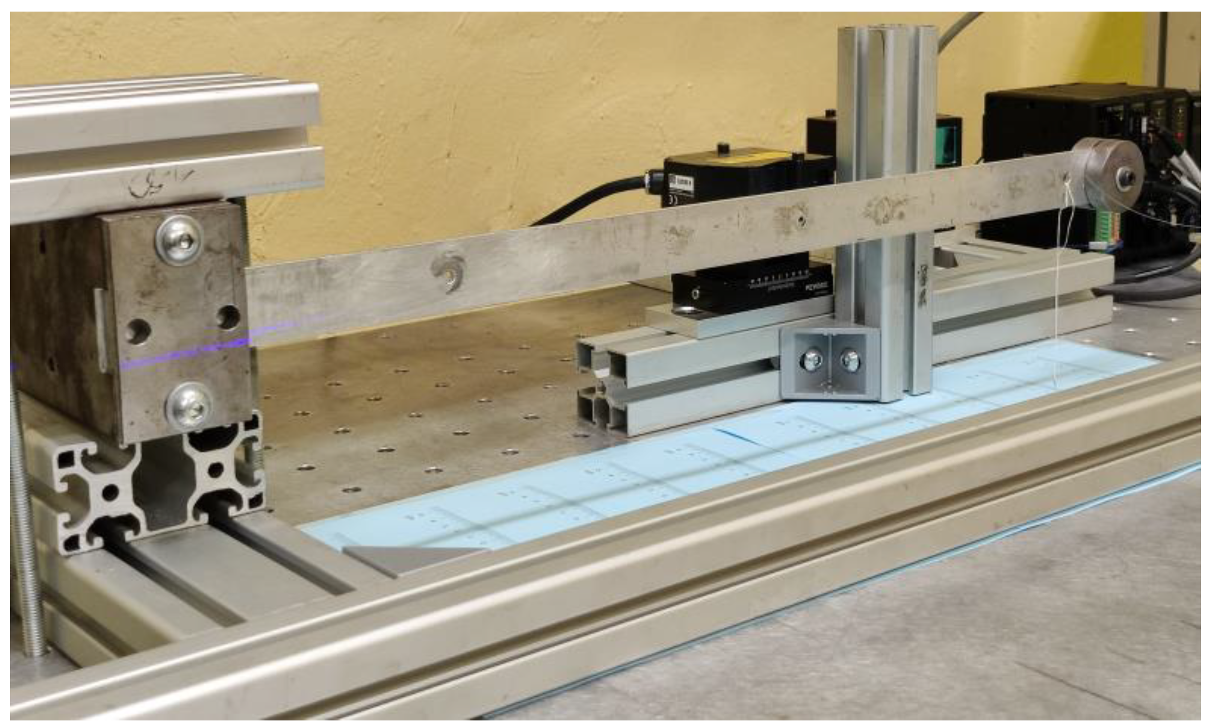
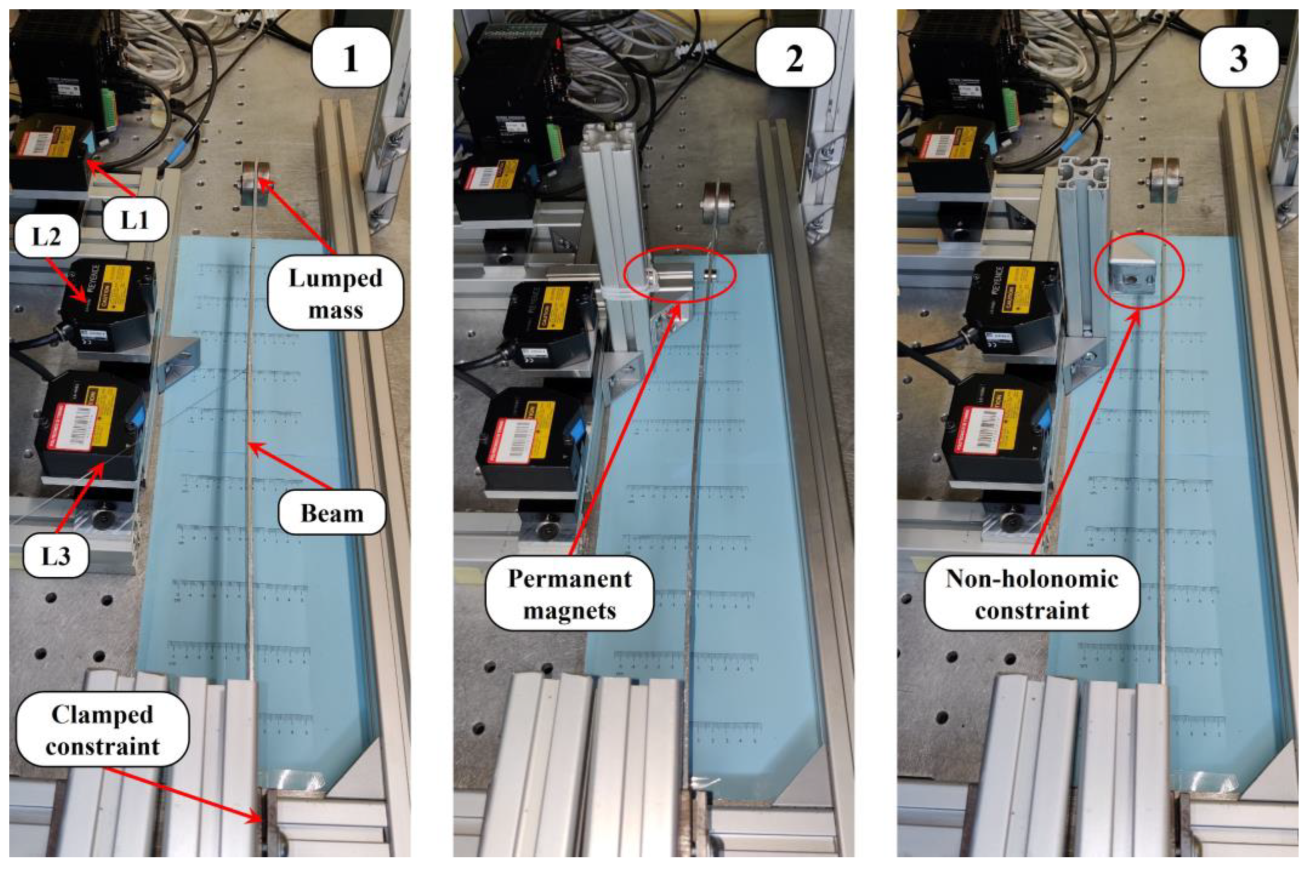
The case study for the detection of nonlinear dynamics using a laser profilometer is the Euler–Bernoulli cantilever beam, reported in Figure 1. It has been tested in three different configurations, as follows:

• The simple and typical clamped-free beam with a lumped mass at the free end. Although a nonlinearity can be present due to a large initial condition displacement, which does not allow the application of small deformation theory, it represents the reference linear case;
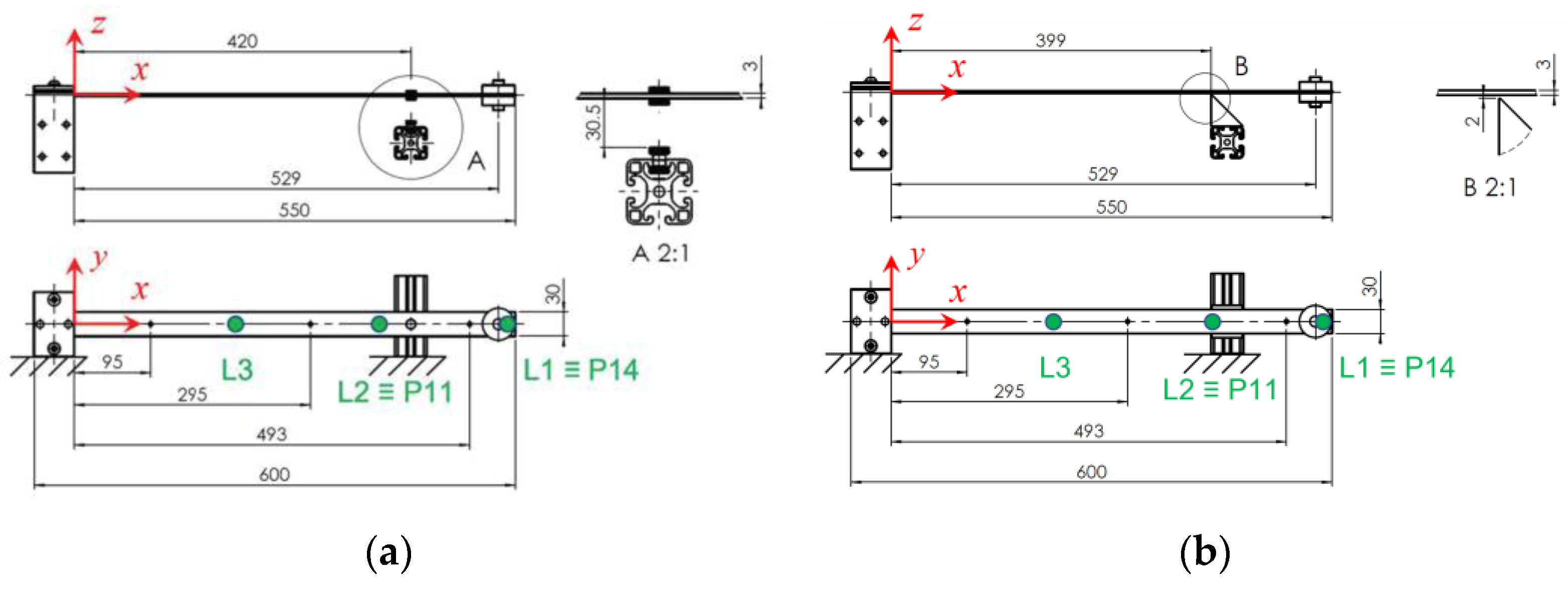
• Two pairs of permanent magnets acting in attraction (#2a) or repulsion (#2r), as in Figure 2a. This introduces a nonlinearity owed to the asymmetric characteristic of the force carried out by these elements;
• A non-holonomic constraint that acts similar to a pin located at a certain distance from the clamp during the time instants in which it is in contact with the beam, as in Figure 2b. This introduces a nonlinearity owed to the contact of the beam with the new introduced constraint.

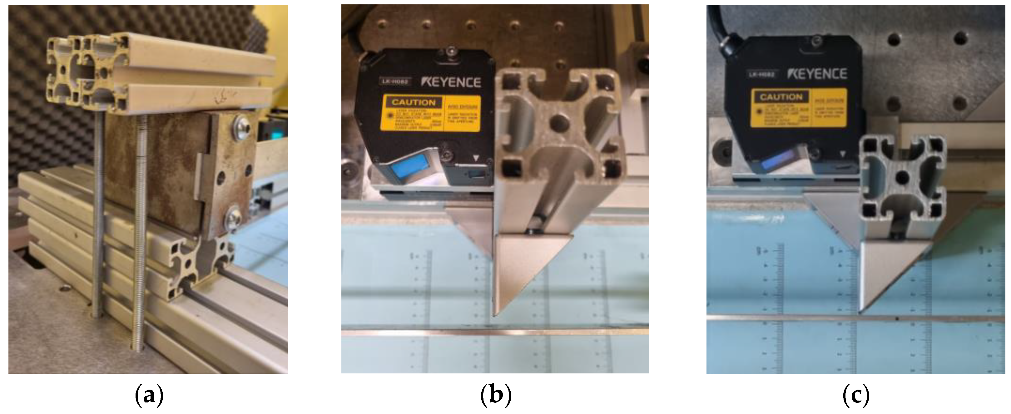
The clamp is composed by two steel parts connected by two screws, as reported in Figure 3a. The four threaded rods that properly lock the system give it great torsional stiffness. Furthermore, the Bosch profile in the upper part of the clamp is in contact only with the biggest part of it, ensuring an ideal clamp since the contact does not give more stiffness to the constraint. On the other side, the contact in the non-holonomic constraint is guaranteed along all the width of the beam, as depicted in Figure 3b,c.

Geometrical and mass properties for beam, clamp, and lumped mass are listed in

Table 1. Weight and property of experimental setup objects.

Item	Weight (g)	Material	Density (kg/m3)	Young Modulus (GPa)	Poisson Ratio (-)
Constraint base	2990.5	Steel	7800	200	0.3
Constraint plate	193.1	Steel	7800	200	0.3
Screws and washers	20.4	Steel	7800	200	0.3
Total constraint	3204.0	Steel	7800	200	0.3
Euler–Bernoulli beam (600 mm × 30 mm × 3 mm)	144.1	Aluminium	2699.2 1	69	0.33
Lumped mass disk	203.37	Steel	8225	200	0.3
Lumped mass fasteners	9.51	Steel	7800	200	0.3
Beam magnets (#2 Ø12h4)	7.1	Nd2Fe14B magnet	7500	-	-
Constraint magnets (#2 Ø12h4 and #1 Ø8h8)	13.3	Nd2Fe14B magnet	7500	-	-
Bosch profiled beams	S 1740 1 R 3040 2	Aluminium	2700	69	0.33

¹ The density of “Euler–Bernoulli beam” is computed directly thanks to the dimensions reported in Figure 2 and considering 2 holes Ø 5.5 and 1 hole Ø 10. ² Bosch profile masses are expressed in unit length for square (S) or rectangular (R) cross-sections.

.

2.2. Instrumentation

Experimental data are acquired using two different sets of hardware. The former consists of three point-lasers, produced by Keyence, of type LK-H082 and LK-H152, while the latter includes the Keyence laser profilometer LJ-X8900, which has the possibility to monitor the displacement of 3200 points at the same time. Lasers are connected to a Siemens SCADAS Mobile, and their sensitivity S is set in the software Siemens Test.Lab in compliance to the margin of error ΔV = 20 V of the output voltage, corresponding to ±10 V. Therefore, the sensitivity is computed as:

$$S=\frac{\Delta V}{2d}$$

(1)

The displacements of the three monitored points of the cantilever beam must stay within the range d given in

Table 2. Point-laser characteristics.

Label	Product Name	Distance D (mm)	Range d (mm)	Sensitivity S (mV/mm)
L1	LK-H152	150	±40	250
L2	LK-H082	80	±18	555.56
L3	LK-H082	80	±18	555.56

, hence their position with respect to the length of the beam has been decided to satisfy this condition, since the greater the distance from the beam the greater the measured displacement will be.

The lasers measure, according to the reference system shown in Figure 2, the displacement of three points, namely:

• a point (L1) at the end of the beam on the lumped mass (x = 545 mm);
• a point (L2) near to the permanent magnets or to the non-holonomic constraint (x = 390 mm);
• a point (L3) between the clamp and the constraints (x = 210 mm).

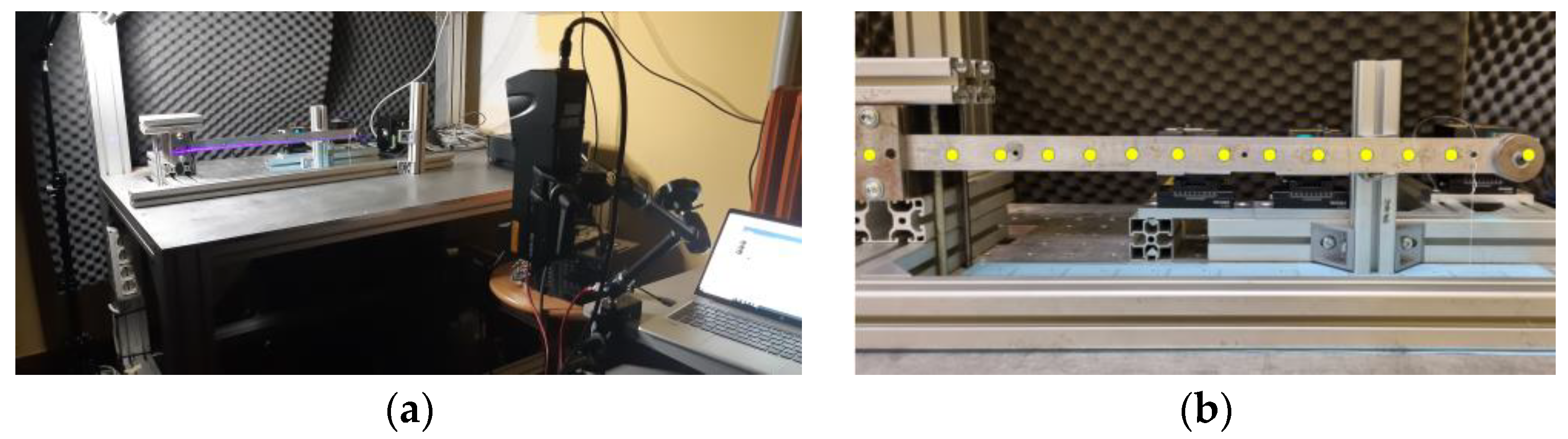
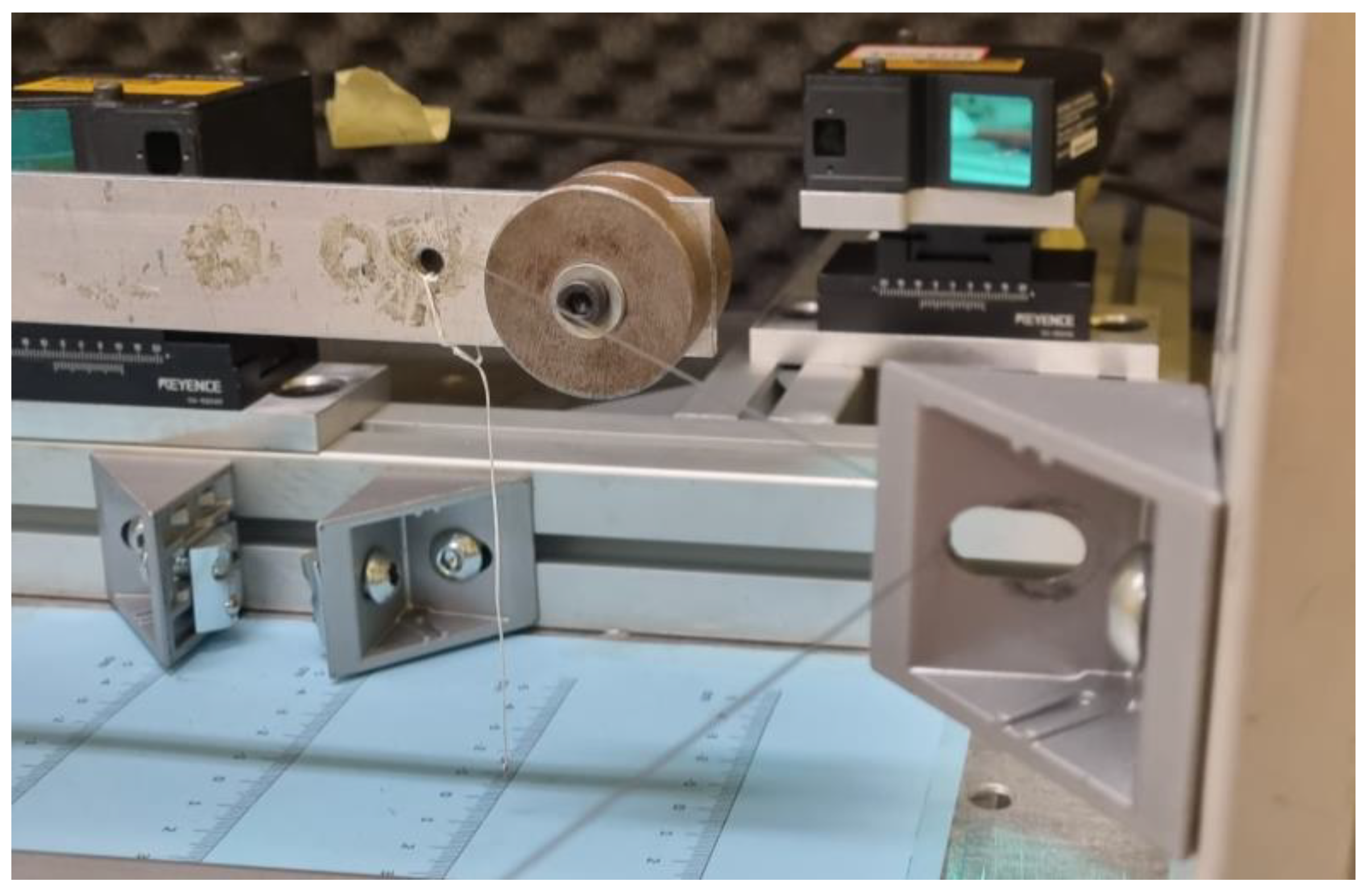
The laser profilometer LX-J8900 is fixed to a rigid table, using the specific support reported in Figure 4a, and projects a laser beam at 980 mm from the cantilever beam to monitor the displacement of 12 fixed points, as displayed in Figure 4b.

By analysing Figure 4b, the measured points are labelled from P1 to P14, and their distance in x direction from the origin of reference system are reported in

Table 3. Coordinates of measured points using a profilometer.

Points	P1	P2	P3	P4	P5	P6	P7	P8	P9	P10	P11	P12	P13	P14
Distance x [mm]	−25	40	80	120	160	200	240	280	320	360	400	440	480	545

.

The point L1, measured with single-point laser, is coincident with the point P14, acquired with the profilometer. For sake of clarity, the profilometer acquisition system is completely independent and not synchronised with the SCADAS Mobile used for the single-point lasers.

2.3. Testing Procedure

The experimental setups, realised to analyse the effect of nonlinearity on the cantilever beam dynamic behaviour in case of magnets in attraction, non-symmetric constraint, and large initial displacement conditions, are reported in Figure 5.

The excitation of the structure is performed with a wire which can be pulled from two different positions:

• the hole near the lumped mass located at 493 mm from the clamp;
• the hole located at 295 mm from the clamp.

In this way, it is possible to separately excite the first two typical bending vibration modes of the Euler–Bernoulli beam: in particular, pulling the wire from the first position, a static deformation equivalent to the 1st bending mode shape is given to the system, while using the second one the static deformation typical of the 2nd bending mode is assigned to the beam. To excite the structure with only a non-null initial displacement, the wire is set with to the desired initial condition (IC): the acquisition software is used to display the chosen IC. Then, the wire is locked and finally cut by a pair of scissors, which allows to have null initial velocity thanks to the instantaneity of the action. Moreover, this procedure has the advantage of being easily repeatable. Additionally, it is important to set the wire along the middle transversal plane of the beam, because, in this way, the torsional modes of the structure are not excited. For sake of clarity, Figure 6 shows how the initial conditions are set.

A sampling frequency f_s = 16,384 Hz is chosen for the single-point lasers, while the maximum sampling frequency of 1000 Hz is chosen for the profilometer acquisition system. Single-point lasers are addressed to high-frequency dynamics measurement, while the profilometer is conventionally adopted for static detections of manufactured products in the production line. Moreover, acquired time histories using the profilometer are limited to 20 s due to acquisition system limits.

From the good agreement of single-point lasers time data and profilometer corresponding point acquisitions comparison, the use of the latter as a reasonable new tool for dynamic tests is proved.

3. Results and Discussion

Several tests have been performed with different configurations of the test rig and Ics. Results of only one acquisition for each testing condition will be shown and discussed in this section. The static deformations of the beam are chosen using the single-point laser software.

3.1. Experimental Data Collection: Time Domain Analysis

In

Table 4. Tests carried out during experimental campaign.

Test	Label	L2 (P11) (mm)	L1 (P14) (mm)	Description
1	BD	−9.95	−16.42	Only beam dynamics
2a	MaD	−14.74	−24.17	Beam dynamics + attractive magnets
2r	MrD	−14.38	−23.61	Beam dynamics + repulsive magnets
3	CD	−11.68	−19.07	Beam dynamics + contact (non-holonomic)

, the most significant tests have been reported, with the IC of points P11 and P14 coincident with the single-point laser L2 and L1, respectively, evaluated from the acquired time histories of Figure 7, Figure 8 and Figure 9.

The BD test is used to evaluate the first natural frequency of the beam in a clamped-free configuration and to properly update the numerical model, which will be used for computing the dynamic properties in case of clamped-pinned-free beam. Moreover, the BD test is used to calibrate the single-point laser offsets to obtain the beam displacement perfectly symmetric with respect to static equilibrium. Only results of the profilometer are analysed, addressing the paper aim. The acquired time history of the BD test is reported in Figure 7.

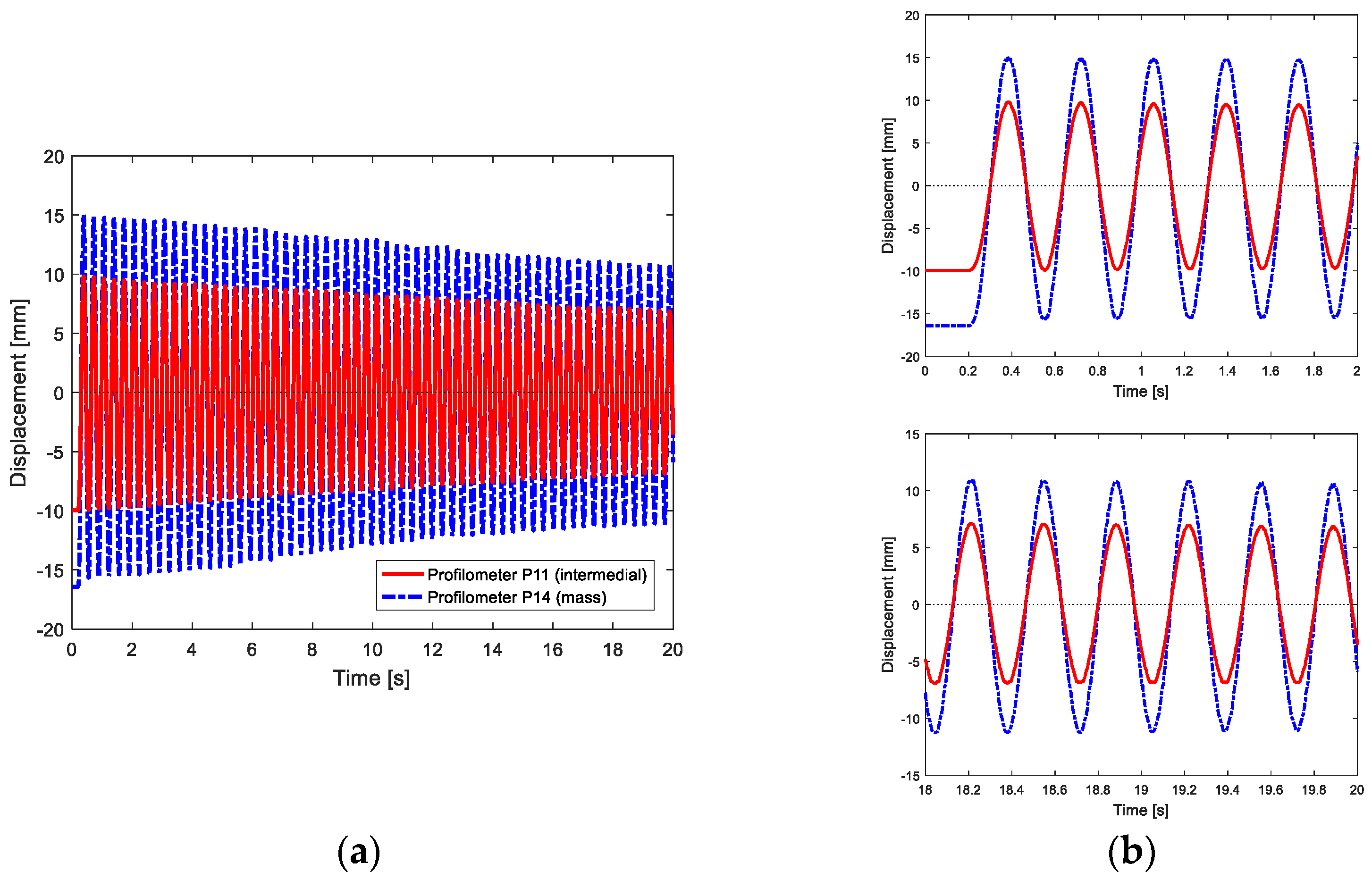
Instead, in Figure 8, the time histories of the MaD test, i.e., the test with magnets in attraction, are shown. From the two details of Figure 8b, it is possible to notice that the points of the beam oscillate around a non-null value, hence a positive drift, due to magnets in attraction and forward the fixed magnets, is present.

Instead, in case of magnets in repulsion, a negative drift would be seen. Similar behaviour but with more extended semi-oscillations along negative displacements is evinced in the MrD test, i.e., the test with magnets in repulsion, not shown in this work.

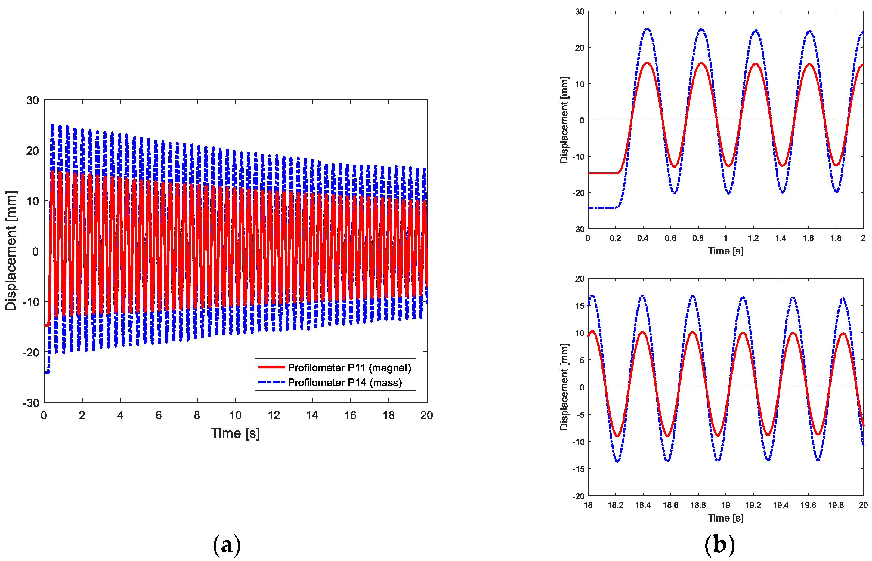
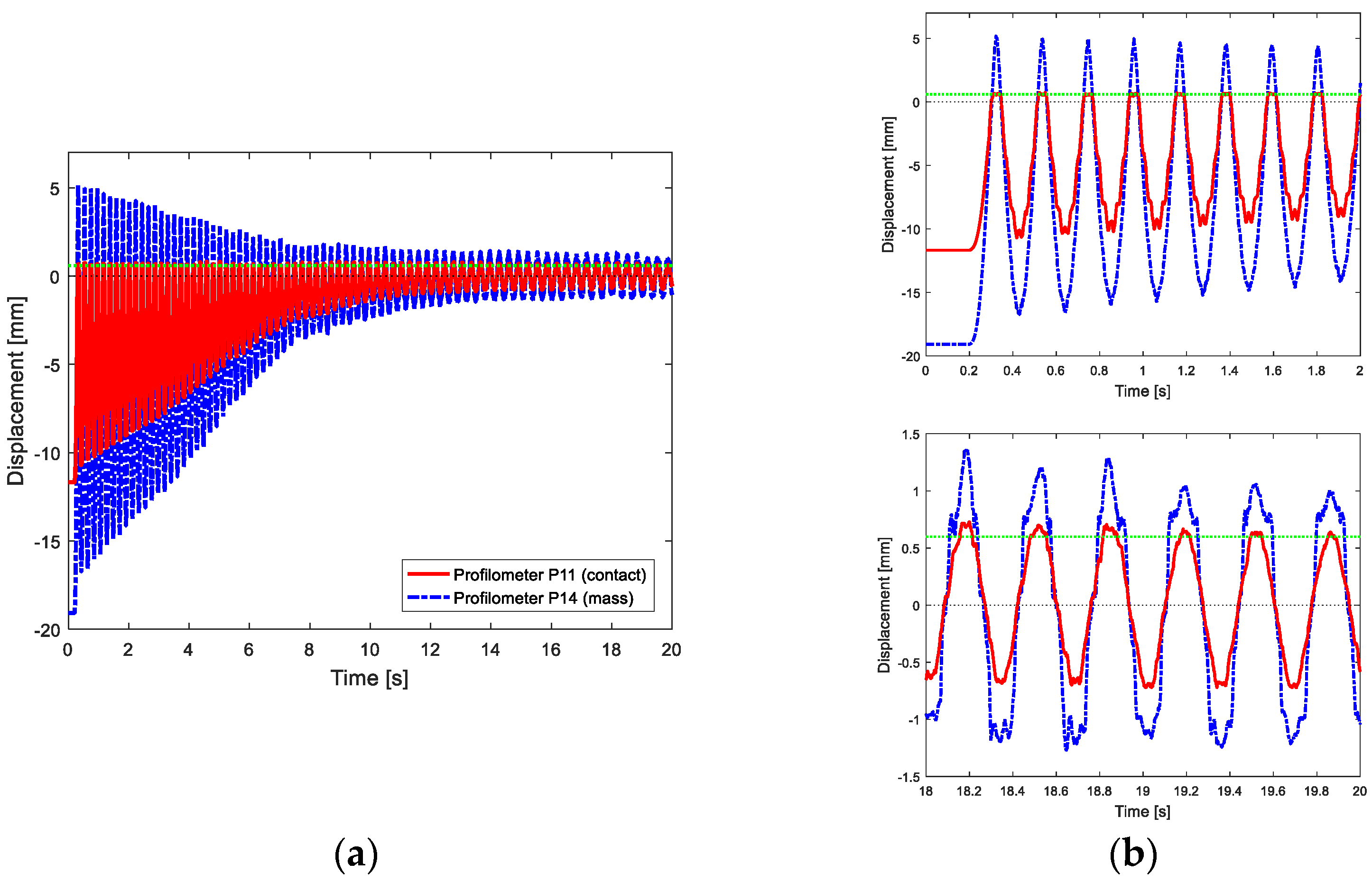
The CD test aims at investigating the nonlinear behaviour in the beam’s dynamics, due to the non-holonomic constraint, which modifies the beam’s boundary conditions, and, consequently, the beam’s natural frequencies.

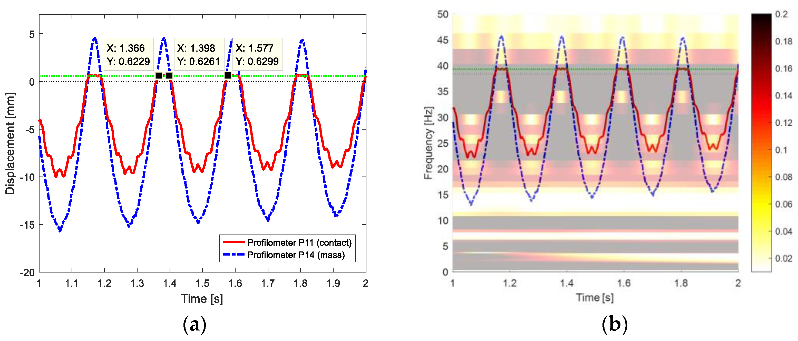
By analysing CD test, the acquired point P11 and P14 time histories are reported in Figure 9. The point P11 corresponds to the contact point of the beam with the non-symmetric constraint, while point P14 is the beam’s free end, where the lumped mass is attached. As it is possible to notice from Figure 9b, the oscillation frequency changes in time, passing from ~4.5 Hz in the first two seconds to ~3 Hz in the last two seconds, in which the contact with the non-holonomic constraint is almost no longer occurring. The point P11 displacement is flat when the contact with the constraint occurs, as indicated by the green horizontal line.

3.2. Post-Processing Methodology

The acquired time histories have been post-processed with a time–frequency analysis, using both Fourier transform and Continuous Wavelet transform with the aim of detecting frequency variations in the time evolution, which can be addressed to nonlinear phenomena.

3.2.1. Fast Fourier Transform Analysis

The time–frequency analysis using Fourier transform consists of a series of frequency analyses on windowed time histories with high overlapping percentages. For time–frequency co-domains directing the Fast Fourier Transform (fft) (Equation (2)) and the inverse the Fast Fourier Transform (ifft) (Equation (3)) relationships for the discrete time signal $x\left(t\right)$ and the signal Fourier transform $X\left(\omega \right)$ are dual and commonly used.

$$X\left(\omega \right)=X\left(x\left(t\right),\omega \right)={\displaystyle {\int }_{-\infty }^{+\infty }{\mathrm{e}}^{\mathrm{i}wt}x\left(t\right)dt}=\mathrm{fft}\left(x\left(t\right)\right)\in ℂ$$

(2)

$$x\left(t\right)={\displaystyle {\int }_{-\infty }^{+\infty }{\mathrm{e}}^{-\mathrm{i}wt}X\left(x\left(t\right),\omega \right)d\omega =}\mathrm{ifft}\left(X\left(\omega \right)\right)=\mathrm{ifft}\left(\mathrm{fft}\left(x\left(t\right)\right)\right)\in ℝ$$

(3)

In the adopted fft and ifft approaches and amplitudes are normalised with the following scale factor $Amp$, where $N$ is the total amount of samples in $x\left(t\right)$, then:

$$Amp=\frac{2}{N-1}$$

(4)

Hence, in the performed FFT time–frequency analysis, a $T_w$ = 4 s has been chosen as time of single windowed signal, with an overlap of 97% and Hamming window.

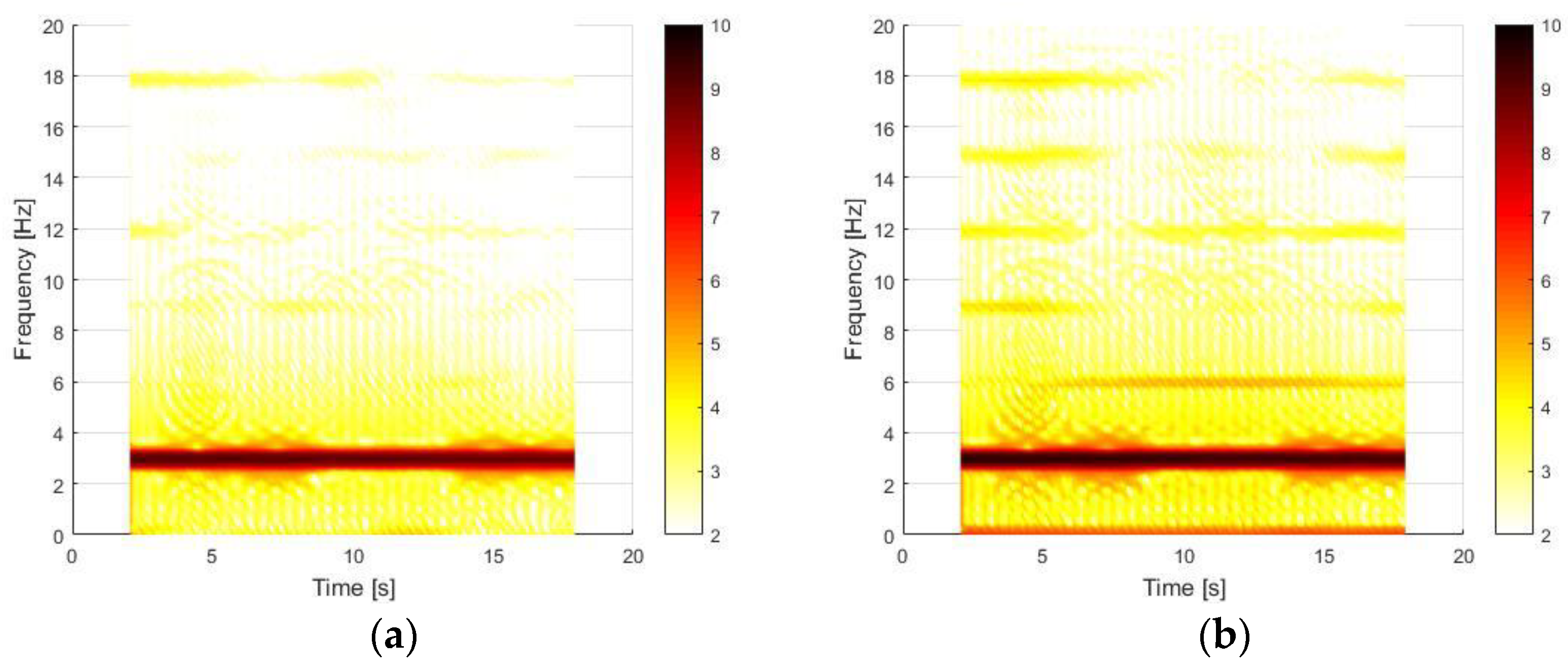
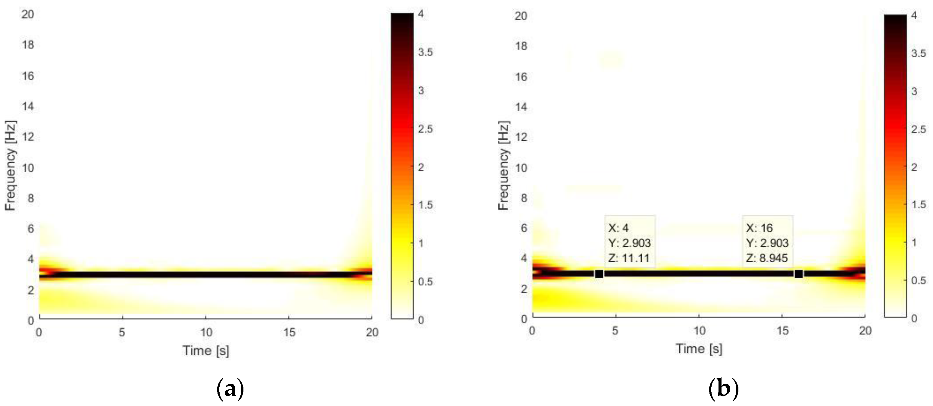
For the BD test shown in Figure 10, a constant harmonic at ~3 Hz is evident, which corresponds to the frequency of the first bending mode in the clamped-free configuration. Instead, the several light horizontal superharmonics are due to leakage phenomena related to Hamming windowing. Moreover, to confirm the softening nonlinearities for large displacements of the clamped-free beam are quite negligible, it is suggested to see the wavelet analysis in the next section.

By analysing Figure 11, processed for MaD test with magnets in attraction, it is possible to notice two nonlinear effects. The former is the presence of the 2nd superharmonics of the fundamental frequency, while the latter is the softening effect. In this configuration, the softening behaviour reduces the global stiffness of the cantilever beam and, consequently, decreases the fundamental frequency and its superharmonics at the beginning of the time history with respect to the end, as noticeable from the markers in Figure 11b. Moreover, the softening effect is more evident when the magnetic restoring force variability is higher, due to larger oscillations of the cantilever beam.

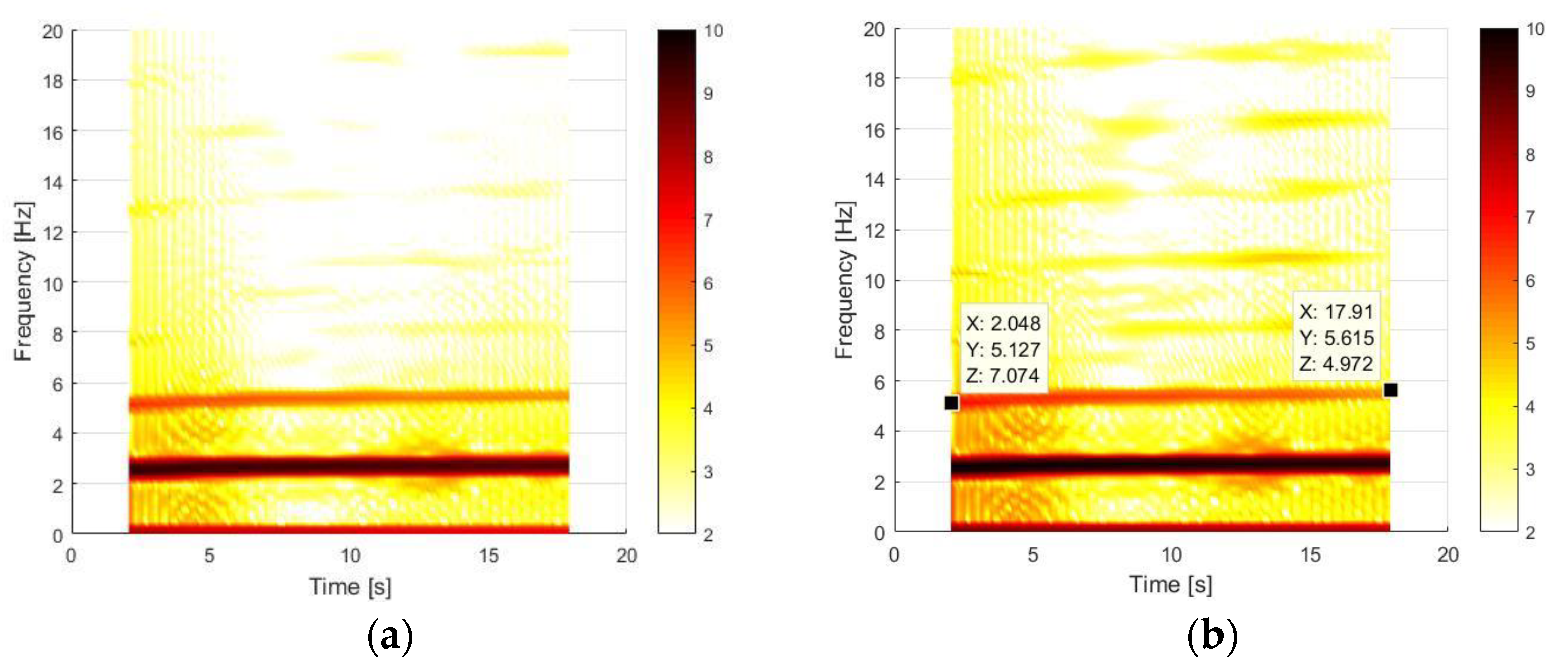
Results of the time–frequency analysis for the CD test are shown in Figure 12. By analysing the mass point P14, reported in Figure 12b, it is evident the 1st frequency transitions with a decrement in time. The 1st natural frequency decreases from a value of ~5 Hz to ~3 Hz when the contact is no longer present. Moreover, the superharmonics of the fundamental natural frequencies are visible in both signals, while, in Figure 12a, it is possible to distinguish the 2nd resonance frequency corresponding to the point near the contact, appearing at ~37 Hz, which agrees with

Table 5. Main frequencies.

Frequency (Hz)	Description
4.7	Mixed frequency
9.4	2nd superharmonics of the mixed frequency
14.1	3rd superharmonics of the mixed frequency
18.8	4th superharmonics of the mixed frequency
37.6	Clamped-free 2nd mode frequency

. This frequency is more evident in Figure 12a since the contact is the main physical cause exciting this second vibrational mode. Hence, the contact corresponds to the point where the beam assumes this behaviour the most.

3.2.2. Continuous Wavelet Method

An alternative time–frequency analysis approach to FFT is the CWT approach. CWT consists of a set of projections $W\left(\tau ,s\right)$ of the signal $x\left(t\right)$ in time $\tau$ and frequency scale $s$ onto rescaled and translated versions of an analysing function $\psi \left(t\right)$, also called a “wavelet” [43,44,45,46]. The projection is translated in a frequency domain integral in which ${\Psi }_{P,\gamma }*\left(\omega \right)$ is the complex conjugate of the Fourier transform of the Morse reference wavelet, and $X\left(\omega \right)$ is the Fourier transform of $x\left(t\right)$.

$$\begin{array}{ll}W\left(\tau ,s\right)& =\frac{1}{s}{\displaystyle {\int }_{-\infty }^{\infty }{\psi }_{P,\gamma }*\left(\frac{t-\tau }{s}\right)x\left(t\right)dt}=\\ & =\frac{1}{2\pi }{\displaystyle {\int }_{-\infty }^{\infty }{\Psi }_{P,\gamma }*\left(s\omega \right)X\left(\omega \right){\mathrm{e}}^{\mathrm{i}wt}d\omega }\end{array}$$

(5)

Hence, the Fourier transform of the generalised Morse wavelet is:

$${\Psi }_{P,\gamma }\left(\omega \right)=U\left(\omega \right)2{\left(\mathrm{e}\frac{{\gamma }^2}{P^2}\right)}^{\frac{P^2}{{\gamma }^2}}{\omega }^{\frac{P^2}{\gamma }}{\mathrm{e}}^{-{\omega }^{\gamma }}$$

(6)

where $U\left(\omega \right)$ is the unit step Fourier transform; $2{\left(\mathrm{e}\frac{{\gamma }^2}{P^2}\right)}^{\frac{P^2}{{\gamma }^2}}$ is a normalising constant; $P^2$ is the time-bandwidth product; and $\gamma$ characterises the symmetry of the Morse wavelet, used in this work for its versatility. By adjusting the time-bandwidth product and symmetry parameters it is possible to obtain wavelets with different behaviours.

Therefore, a time–frequency analysis of the evolution of the measured points is performed with CWT based on Morse wavelets.

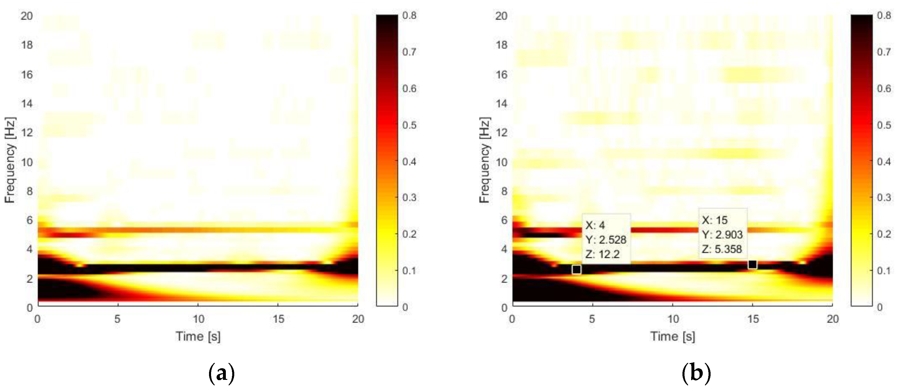
The use of CWT does not provide further details for the BD test, where the beam is analysed in clamped-free conditions. Results reported in Figure 13 are similar to the time–frequency analysis using FFT reported in Figure 10. The two labels at the beginning and at the end of time history confirm the nonlinear effects due to large oscillations are negligible, since the frequency is the same of the first bending mode at ~3 Hz.

Regarding the MaD test, the softening effect that decreases the starting value of each harmonic when the amplitude of oscillations is higher is more evident respect to the FFT analysis, where overlapping is applied to the time history, with a subsequential averaging of results.

From Figure 14a, the 2nd and the 3rd superharmonics can be noticed in the first 4 s. This is the confirmation that a nonlinear magnetic force in the equation of motion, if developed up to the 3rd term, completely describes the action of the magnets. The signal contributions at a near zero frequency at the beginning and end of time history are related to the wavelet cone of influence, which shows where the edge effects of the CWT become significant, hence this region should be excluded from the analysis. Moreover, by changing wavelet parameters to have a better frequency resolution, the cone of influence changes as well.

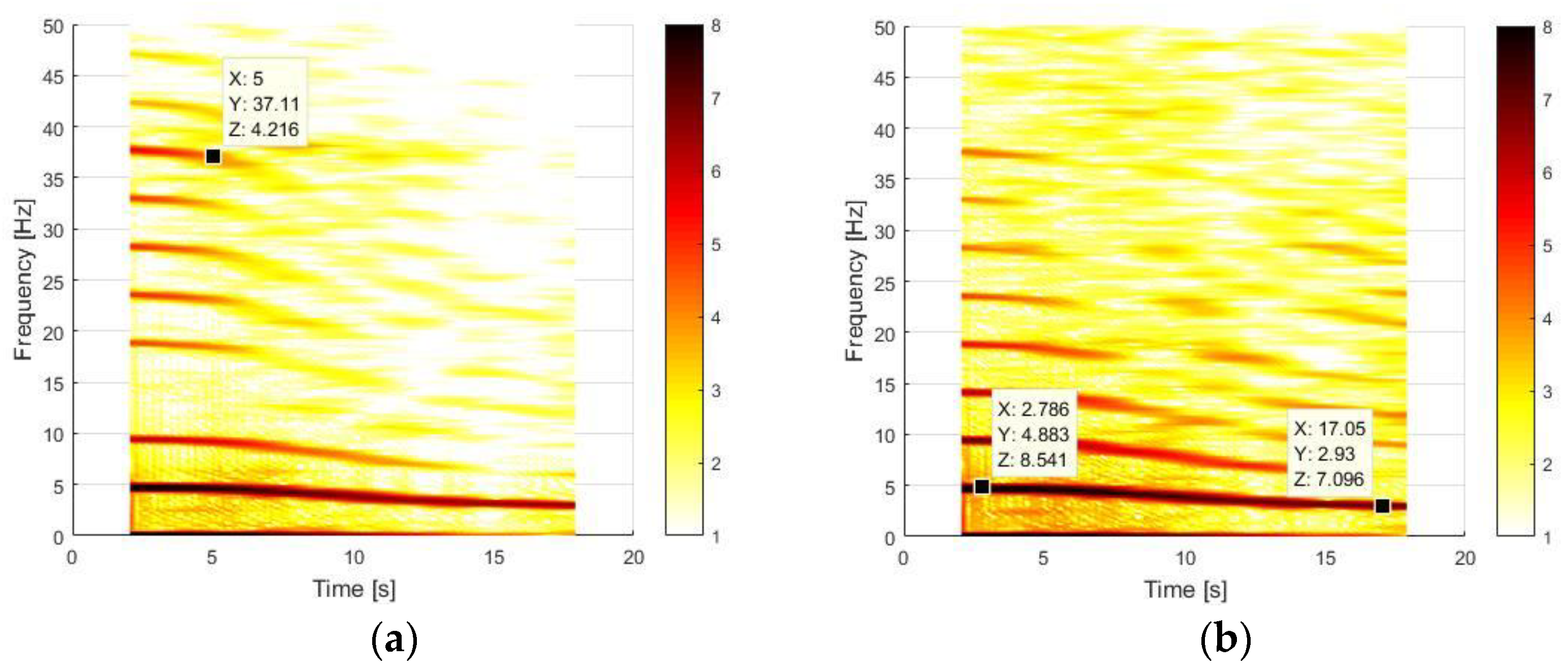
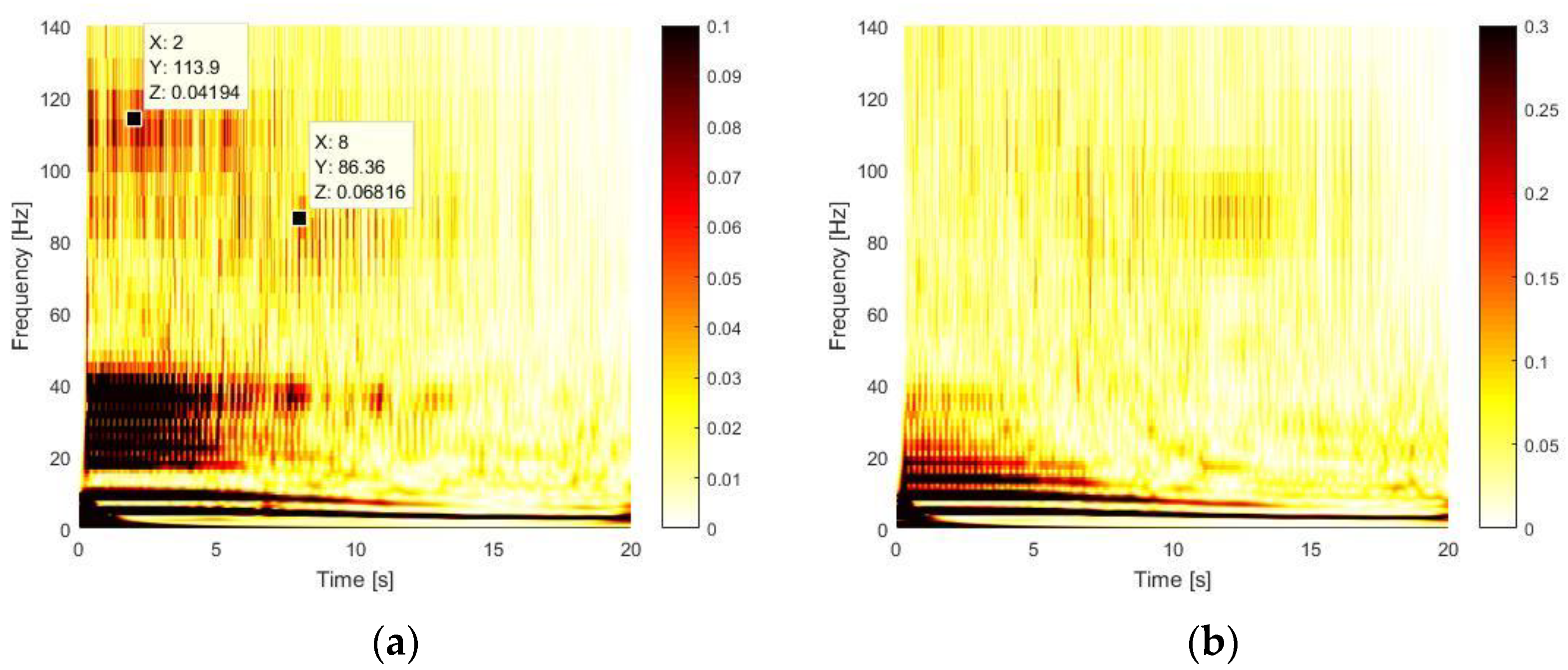
The application of the CWT method to the CD test returns the most interesting results, as shown in Figure 15. From a global point of view, several high spectral contents can be noticed at different frequencies. The markers in Figure 15a, which represent the time–frequency analysis for the contact point, show a frequency contribution at ~86 Hz and ~114 Hz, which are the 2nd natural frequency of the system in clamped-pinned-free conditions and the and 3rd natural frequency of the system in a clamped-free configuration, as stated in Table 5.

For a deeper analysis, a detail of the time interval of 1 ÷ 5 s and in the frequency range of 0 ÷ 50 Hz is shown for both P11 (contact) and P14 (mass), as reported below.

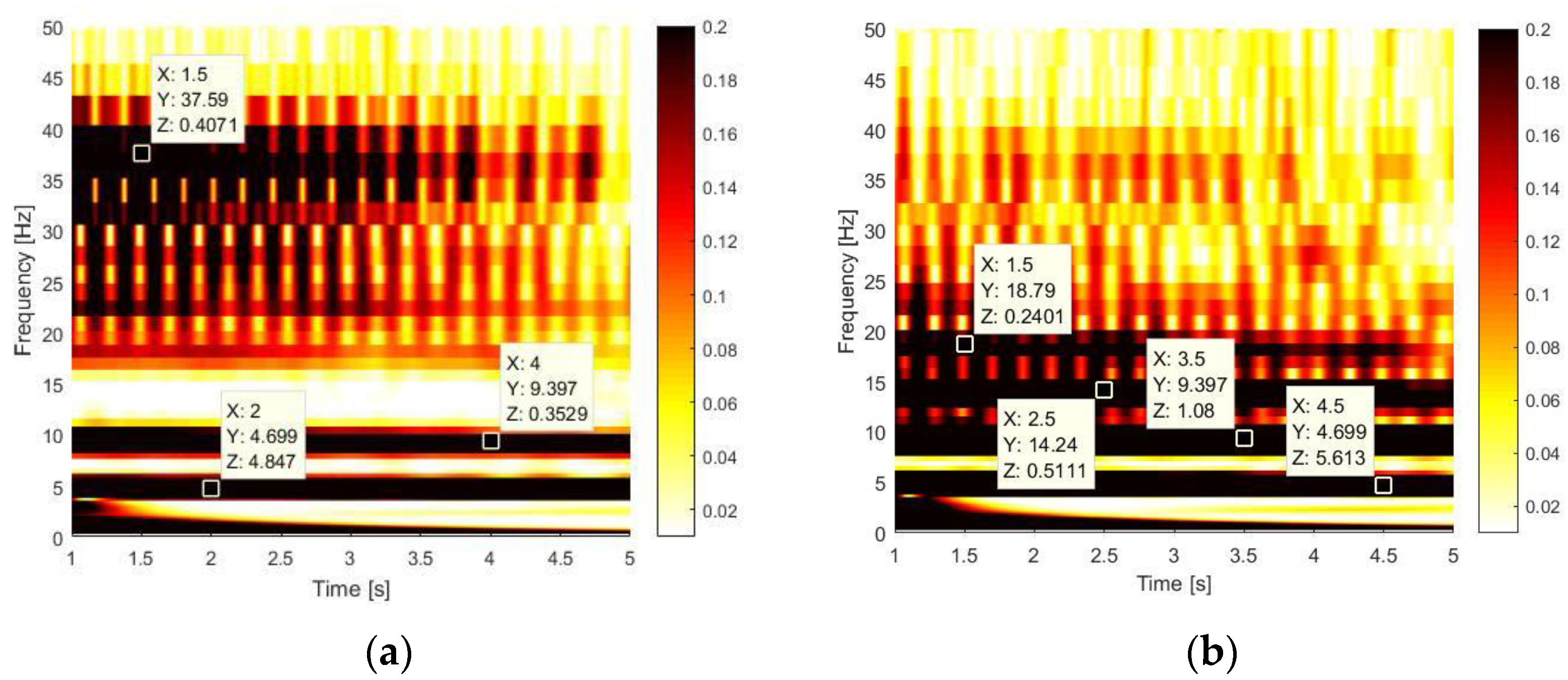
In Figure 16, there is the evidence of some relevant frequency contents.

For sake of clarity, a list of all marked frequencies, also summarised in Table 5, is provided to investigate the system dynamics in frequency domain:

• ~4.7 Hz identifies a mixed frequency, which is a weighted average of the first natural frequencies of the clamped-free and clamped-pinned-free configurations over the time in each configuration. This is confirmed by the periods corresponding to these bending modes which are larger than the contact time of about 0.032 s, as shown in Figure 17;
• ~9.4 Hz is the 2nd superhamonics of the mixed frequency at ~4.7 Hz. It is usual to have superharmonics of even order even if a magnet is not present, indeed this contribution comes from the truncation of the displacement when there is the contact;
• ~14.1 Hz is the 3rd superharmonics of the mixed frequency of ~4.7 Hz. It is not visible on the contact since it is stopped by the angular profile which does not allow the nonlinearity to locally develop its effect, since this displacement is not as describable as at the mass point with an expansion mainly characterised by terms of 3rd order;
• ~18.8 Hz is the 4th superhamonics of the mixed frequency at ~4.7 Hz;
• ~37.6 Hz is related to the 2nd bending mode of beam in clamped-free configuration.

The time–frequency analysis performed at the mass point in Figure 16b shows a frequency bouncing between the 2nd mode of the clamped-free (~37.6 Hz) and the 2nd superharmonics of the mixed frequency (~9.4 Hz). On the other side, the time–frequency analysis performed at the contact point in Figure 16a shows a frequency bouncing between the 2nd mode of the clamped-free system (~37.6 Hz) and the 4th superharmonics of the mixed frequency (~18.8 Hz). The lower frequency value of the bouncing changes since the time–frequency analysis of the measurements performed at the contact point does not show the behaviour related at the 3rd superharmonics of the 1st mode because of the asymmetry of the contact, hence the closer and higher frequency is the 4th superharmonics of the first mode at ~18.8 Hz.

Figure 17 is used to clarify that the contact of the beam with the constraint during the first fully acquired oscillation lasts from 1.366 s to 1.398 s, while the complete oscillation ends at 1.577 s.

Therefore, the value of ~4.7 Hz derives from Equations (7) and (8).

$$f_{mean}=2.97x+13.88\left(1-x\right)=4.627\mathrm{Hz}$$

(7)

which is a weighted average of values of the fundamental frequencies of the clamped-free and clamped-pinned-free configurations, i.e., 2.97 Hz and 13.88 Hz, respectively, as reported in Table 6. The x value corresponds to the time in which the beam is not in contact, and it is computed with the instants marked in Figure 17a and is equal to:

$$x=\frac{1.577-1.398}{1.577-1.366}=84.83\%$$

(8)

3.3. Numerical Modelling

Due to the large variety of nonlinearities, a suitable choice of methods is mandatory to emphasize their contribution in the system dynamics according to the scale of the effect with respect to the macroscopic system behaviour.

In this scenario, MOR methods are affirmed techniques, which can strongly reduce the computational cost mainly acting on the DoF amount.

In case of magnet interaction, the magnet continuous displacement characteristics induces a smooth behaviour in dynamics. Eventually, the macroscopic system dynamics can be linearised around the static equilibrium position [51]. Instead, if the nonlinearity is not negligible, the system can be reduced by single DoF modelling and a Hilbert transform is suitable for the study of the nonlinearity.

Non-smooth nonlinearities [52] such as contact phenomena have been successfully described with model-based MOR methods. In this scenario, the identification of different linearised configurations of the system and the description of the transition through them as convolutions in time through the application of boundary conditions on reduced models is a successful strategy. Therefore, the Multi-Phi approach is introduced and the configurational nature of the system with non-holonomic constraints is demonstrated by the identification of its configurations with finite element model modal analysis depicting their major natural frequencies, which are also observed in previous time–frequency analyses.

3.3.1. Effect of Magnets on a Cantilever Beam: Hardening or Softening Behaviours

The mechanical and dynamic properties of the cantilever beam resulting from the numerical model are used to develop a single DoF system model that approximates the first bending mode of the numerical model. Thus, the analytical model is used to investigate the nonlinear effect given by the magnets when they are used in attraction or repulsion.

The elasto-magnetic system represented in Figure 2a can be described by the following nonlinear equation:

$$m\ddot{z}+k\left(z-z_e\right)+F_m=0$$

(9)

where $z$ is the position of the beam; $z_e$ is the static equilibrium; $F_m$ is the magnetic force which can be attractive or repulsive, depending on the sign positive or negative, respectively, and it is modelled through the empirical formula of Equation (10); while $m$ and $k$ are the equivalent mass and stiffness, given by Equation (11):

$$F_m=\pm \frac{A}{{\left(1-\frac{z}{B}\right)}^n}$$

(10)

$$\begin{array}{c}m=m_l+m_b\\ k=m{\left(2\pi f_n\right)}^2\end{array}$$

(11)

where parameters $A$, $B$, and $n$ may be evaluated through magnetic models based on equivalent currents method [33,34,53], while $m_l$ and $m_b$ are the lumped mass and the beam mass participating to the first mode, equal to one third of the total one (without considering the clamped part), which, according to Table 6, has a natural frequency of $f_n$ = 2.97 Hz.

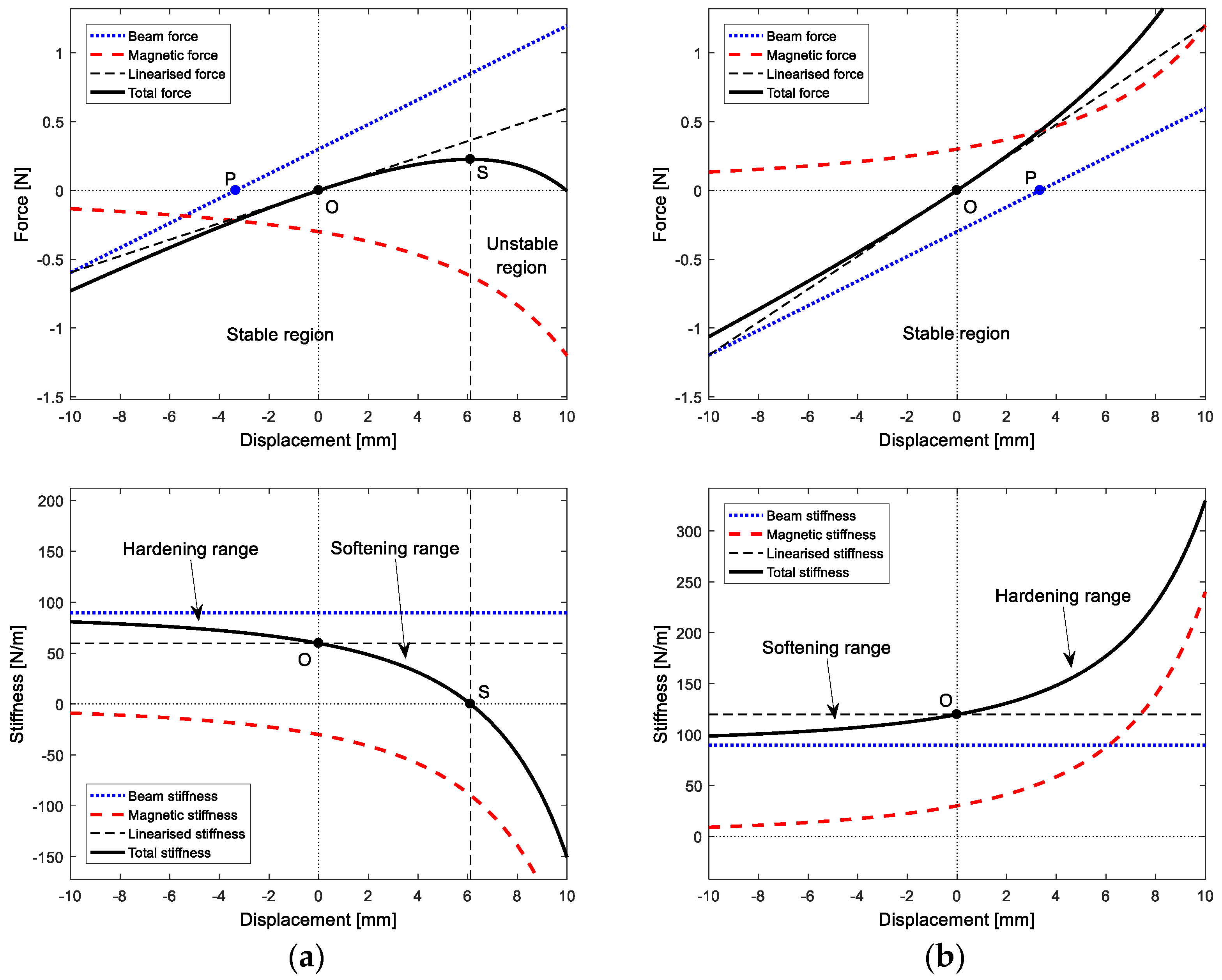
Figure 18 shows on the top the forces acting on the system, namely, the elastic force of the beam, the magnetic force with a different sign in case of attraction (a) or repulsion (b), and also the total force because of the superposition of these two effects. Points O corresponding to null displacement identify beam static positions in attractive and repulsive magnetic configurations. Since points P correspond to the equilibrium beam position without magnets, offsets between the respective cases with and without magnets can be noticed. The two static magnetic configurations are reached when magnetic and elastic forces reach opposite values that balance each other.

Secondly, point S of attraction magnet configuration corresponds to the transition between the stable region and unstable region. The attractive magnetic force is high enough to interrupt beam oscillation because magnets attach each other when the analysed beam point reaches this unstable region. Point S corresponds to the balance of elastic and magnetic stiffness reached when the derivative of the total force is null, i.e., when the elastic and magnetic stiffness, shown on the bottom of Figure 18, assume opposite values. Consequently, this unstable region is not present in the repulsion magnetic case since the two stiffnesses never assume opposite values, thus the system is always stable.

Finally, by analysing total stiffness trends it is possible to identify softening and hardening behaviours caused by the nonlinearities due to magnets: hardening occurs when the total stiffness is higher than the respective linearised value, while, in the opposite case, the behaviour is softening. Both attraction and repulsion cases show two regions of softening and hardening, hence the global dynamic behaviour of the beam is a consequence of which one of these two overcomes the other during one oscillation period. The system with attraction magnets shows softening behaviour for positive displacements and hardening for negative ones.

The system with repulsion magnets shows softening behaviour for positive displacements and hardening for negative ones. The overall effects of attraction and repulsion magnetic system are, respectively, softening and hardening behaviours, as highlighted by frequency analyses. To confirm the results obtained with both time–frequency analyses about the nonlinear characteristics of the system, the Hilbert transform is used, according to the non-parametric Feldman’s method [49,50].

3.3.2. Hilbert Transform

With reference to the methodology developed by Hilbert [49], recalling the approach that has already been used in [50], the unforced behaviour of a nonlinear mechanical single degree of freedom (sdof) system can be expressed in the form:

$$m\ddot{z}\left(t\right)+c\left(t\right)\dot{z}\left(t\right)+k\left(t\right)z\left(t\right)=0$$

(12)

where the nonlinear damping coefficient $c\left(t\right)$ and the nonlinear stiffness coefficient $k\left(t\right)$ depend on displacement and velocity. The linear canonical form of the equation of motion is written as follows:

$$\ddot{z}\left(t\right)+2\zeta \left(t\right){\omega }_n\left(t\right)\dot{z}\left(t\right)+{\omega }_n^2\left(t\right)z\left(t\right)=0$$

(13)

where the non-dimensional damping factor $\zeta \left(t\right)$ and the natural frequency ${\omega }_n\left(t\right)$ are time dependent. By considering the definition of the complex analytic signal of $z\left(t\right)$, expressed in exponential form, it holds:

$${\rm Z}\left(t\right)=z\left(t\right)+\mathrm{i}\tilde{z}\left(t\right)=A\left(t\right){\mathrm{e}}^{\mathrm{i}\Psi \left(t\right)}$$

(14)

where $\tilde{z}\left(t\right)$ is the Hilbert transform of the real signal $z\left(t\right)$. The real envelope function $A\left(t\right)$ and the real instantaneous phase function $\Psi \left(t\right)$, which are both time-dependent, result in, respectively:

$$\begin{array}{l}A\left(t\right)=\sqrt{z{\left(t\right)}^2+\tilde{z}{\left(t\right)}^2}\\ \Psi \left(t\right)={\tan }^{-1}\frac{\tilde{z}\left(t\right)}{z\left(t\right)}\end{array}$$

(15)

where $\omega \left(t\right)=\dot{\Psi }\left(t\right)$ is the instantaneous angular frequency. The time-dependent damping $\zeta \left(t\right)$ and natural frequency ${\omega }_n\left(t\right)$ functions are related to the envelope and phase functions through the relations:

$$\begin{array}{l}\zeta \left(t\right)=-\frac{1}{{\omega }_n}\left(\frac{\dot{A}}{A}+\frac{\dot{\omega }}{2\omega }\right)\\ {\omega }_n\left(t\right)=\sqrt{{\omega }^2+\frac{\dot{A}\dot{\omega }}{A\omega }+2\frac{{\dot{A}}^2}{A^2}-\frac{\ddot{A}}{A}}\end{array}$$

(16)

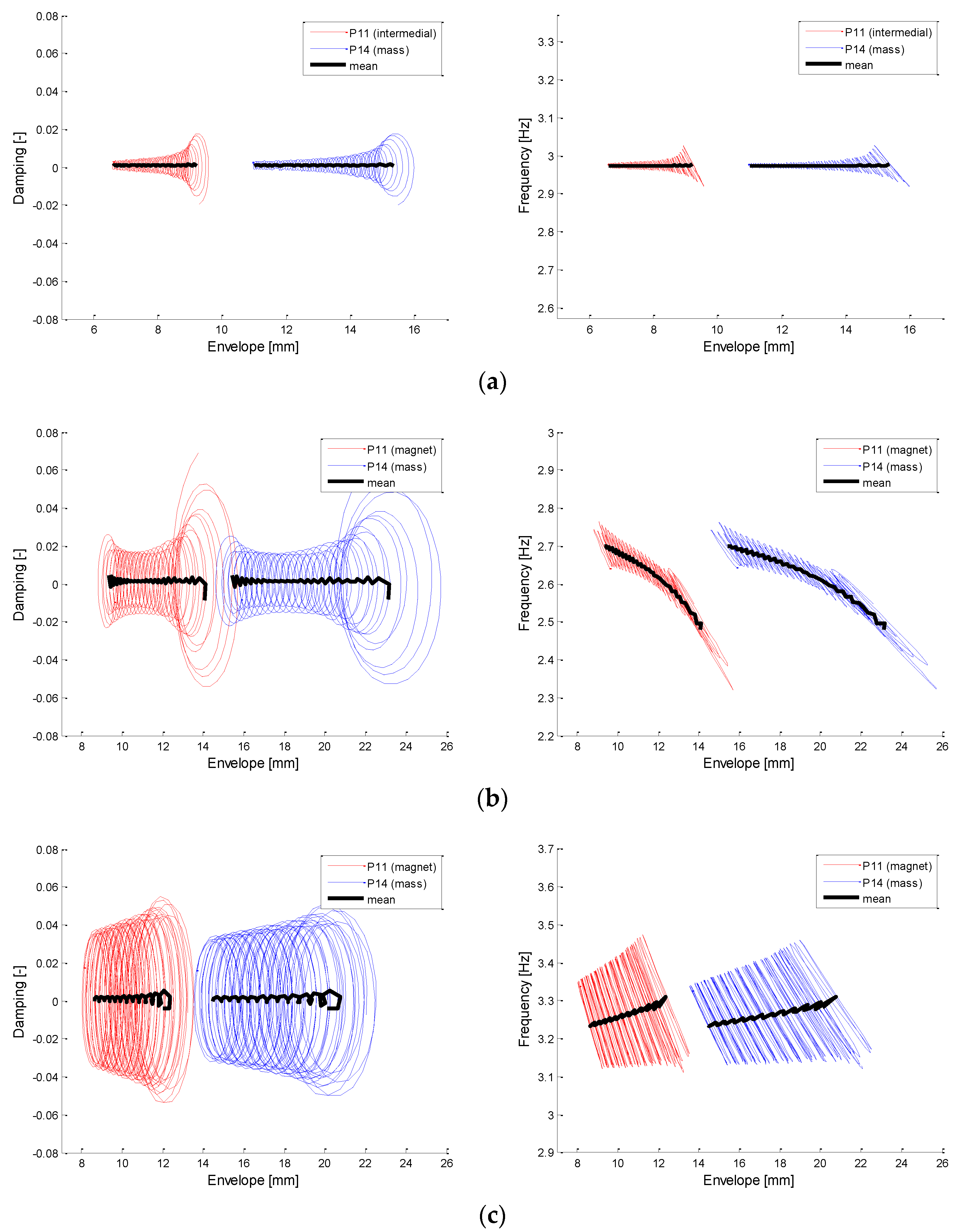
The Hilbert transform is applied to the BD (simple clamped-free beam case), MaD (beam with attraction magnetic configuration), and MrD (beam with repulsive magnetic configuration) tests.

The outcomes in Figure 19 (left) show the correlation between envelope and damping trends, highlighting how the latter are not characterised by wide variations. A similar behaviour has been observed in as small-scale application i.e. the Levitron © device, in which the contact between moving and fixed parts due to constraints is absent [54]. Furthermore, Figure 19 (right) shows the correlation between frequency and envelope trends that confirm the linear, softening, and hardening behaviours, respectively, caused by the presence of magnetic nonlinearities, in similarity with other applications such as Levitron ©.

Red and blue trajectories correspond to points P11 and P14, respectively, demonstrating the filtering effects of the free mass with respect to points closer to the nonlinear effect. The natural frequency for smaller oscillations, hence for smaller envelopes, converges to the natural frequency of the magnetic configurations that are linearised about the respective equilibrium positions, demonstrating the nature of the nonlinear characteristics, which appears to depend on displacement.

3.3.3. Multi-Phi Approach

A numerical model of the Euler–Bernoulli cantilever beam, with about 400 DoFs, has been developed using LUPOS [41,42] for the validation of the experimental campaign. Two linearised models have been developed and tuned to describe the nonlinear dynamics in case of non-holonomic constraints. Mass and material properties, according to Table 1, have been assigned to the different components of the experimental setup. Real modal analysis is used for computing natural frequencies and mode shapes of the system in the two different configurations:

• beam clamped free;
• beam clamped pinned free.

Considering the two configurations as two linear systems, for a generic $l$ linear system, the equations of motions are described by Equation (17), which is written for active DoFs $n$, after which the boundary conditions or other reductions are applied:

$$M^{\left(l\right)}{\ddot{x}}^{\left(l\right)}+C^{\left(l\right)}{\dot{x}}^{\left(l\right)}+K^{\left(l\right)}{x}^{\left(l\right)}=f\left(t\right)$$

(17)

where $x^{\left(l\right)},{\dot{x}}^{\left(l\right)},{\ddot{x}}^{\left(l\right)}\in {ℝ}^{n\mathrm{x}1}$ are the system displacements, velocities, and accelerations, respectively; $M^{\left(l\right)},C^{\left(l\right)},K^{\left(l\right)}$ are the mass, damping, and stiffness matrices of the considered $l$ linear system; and $f\left(t\right)$ is the time depending external forcing function applied to the system. Neglecting static generalised external forces, and assuming a proportional damping matrix, Equation (17) can be written using the homogeneous expression:

$$M^{\left(l\right)}{\ddot{x}}^{\left(l\right)}+K^{\left(l\right)}{x}^{\left(l\right)}=0$$

(18)

Hence, modal analysis is performed on each level of the system, i.e., in clamped-free and clamped-pinned-free conditions of the CD test. For each level, to evaluate a non-null stationary oscillating behaviour, a generalised exponential solution is assumed, as in Equation (19):

$$\{\begin{array}{c}\begin{array}{l}x=x_0{\mathrm{e}}^{\mathrm{i}\omega t}\\ \dot{x}=\mathrm{i}\omega x_0{\mathrm{e}}^{\mathrm{i}\omega t}\\ \ddot{x}=-{\omega }^2{x}_0{\mathrm{e}}^{\mathrm{i}\omega t}\end{array}\end{array}$$

(19)

Hence, time is separable and erasable from the equation:

$$\left(K-{\omega }^{2}M\right)x_0=0$$

(20)

Apart the trivial solution $x_0=0$ that corresponds to the static undeformed condition, Equation (20) presents non-null solutions when the rank is non-full, hence an eigenproblem is definable to evaluate eigenvalues ${\omega }_r^2$ and eigenvectors ${\mathsf{\phi }}_r$, finding the non-null solutions of the eigenproblem in Equation (21) by the means of Equation (22):

$$\left(K-{\omega }_r^{2}M\right){\mathsf{\phi }}_r=0$$

(21)

$$\det \left(K-{\omega }^{2}M\right)=0$$

(22)

Thus, for each eigenvalue ${\omega }_r^2$, its corresponding eigenvector ${\mathsf{\phi }}_r$ is computed and then normalised to unitary modal mass ${\Phi }_r$. Equation (21) can be written as:

$$\left(K-{\omega }_r^{2}M\right){\Phi }_r=0\hspace{0.17em}\mathrm{or}\hspace{0.17em}K\Phi =M\Phi \mathrm{diag}\left({\mathsf{\omega }}_r^2\right)$$

(23)

Assuming a proportional damping matrix, the modal superposition of physical coordinates $x^{\left(l\right)}$ results in:

$$\{\begin{array}{l}{x}^{\left(l\right)}={\Phi }^{\left(l\right)}{\mathsf{\eta }}^{\left(l\right)}\left(t\right)+{x_{\infty }}^{\left(l\right)}\\ {\dot{x}}^{\left(l\right)}={\Phi }^{\left(l\right)}{\dot{\mathsf{\eta }}}^{\left(l\right)}\left(t\right)\\ {\ddot{x}}^{\left(l\right)}={\Phi }^{\left(l\right)}{\ddot{\mathsf{\eta }}}^{\left(l\right)}\left(t\right)\end{array}$$

(24)

where ${\Phi }^{\left(l\right)}\in {ℝ}^{n\times r_l}$ and ${\mathsf{\eta }}^{\left(l\right)}\in {ℝ}^{r_l\times 1}$. In Equation (24), the addition of ${x_{\infty }}^{\left(l\right)}$, called asymptotic configuration, is necessary whenever the set of mode shapes is used to simulate the system evolution cannot describe the system state because of non-null boundary conditions. It is considered function of time because it depends on the linearised system considered at each time instant. It is determined, using Guyan reduction [55], by means of Equation (25), where $x_k$ represents the boundary conditions (known DoFs), while $x_u$ represents the not constrained DoFs (unknown).

$$\{\begin{array}{l}{x}_{\infty }=\left[\begin{array}{c}-{\left(K_{uu}^{\left(l\right)}\right)}^{-1}{K}_{uk}^{\left(l\right)}\\ I\end{array}\right]x_k\\ {\dot{x}}_{\infty }=0\end{array}$$

(25)

The evolution of the full system, during the span of time in which the $l$-th configuration dynamics is triggered, depends only by the transition to another level occurring when a certain kinematic condition is respected. The transition is governed by Equation (26), in which the initial conditions of the modal coordinates of the level $m$ are described by means of the final conditions of modal coordinates of the level $l$:

$$\{\begin{array}{l}{\mathsf{\eta }}_{m,0}={\Phi }_m^{-1}\left({\Phi }_l{\mathsf{\eta }}_{l,end}+x_{\infty ,l}-x_{\infty ,m}\right)\\ {\dot{\mathsf{\eta }}}_{m,0}={\Phi }_m^{-1}{\Phi }_l{\dot{\mathsf{\eta }}}_{l,end}\end{array}$$

(26)

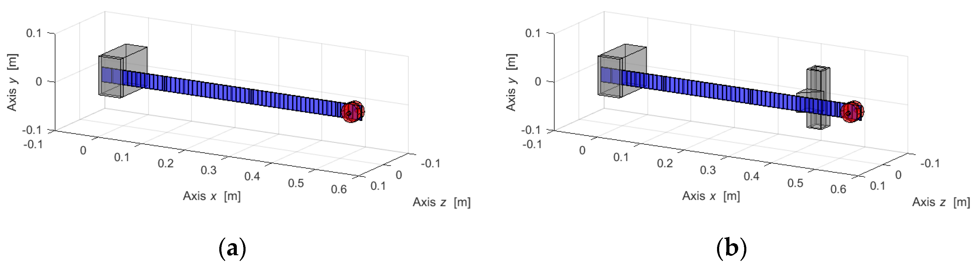
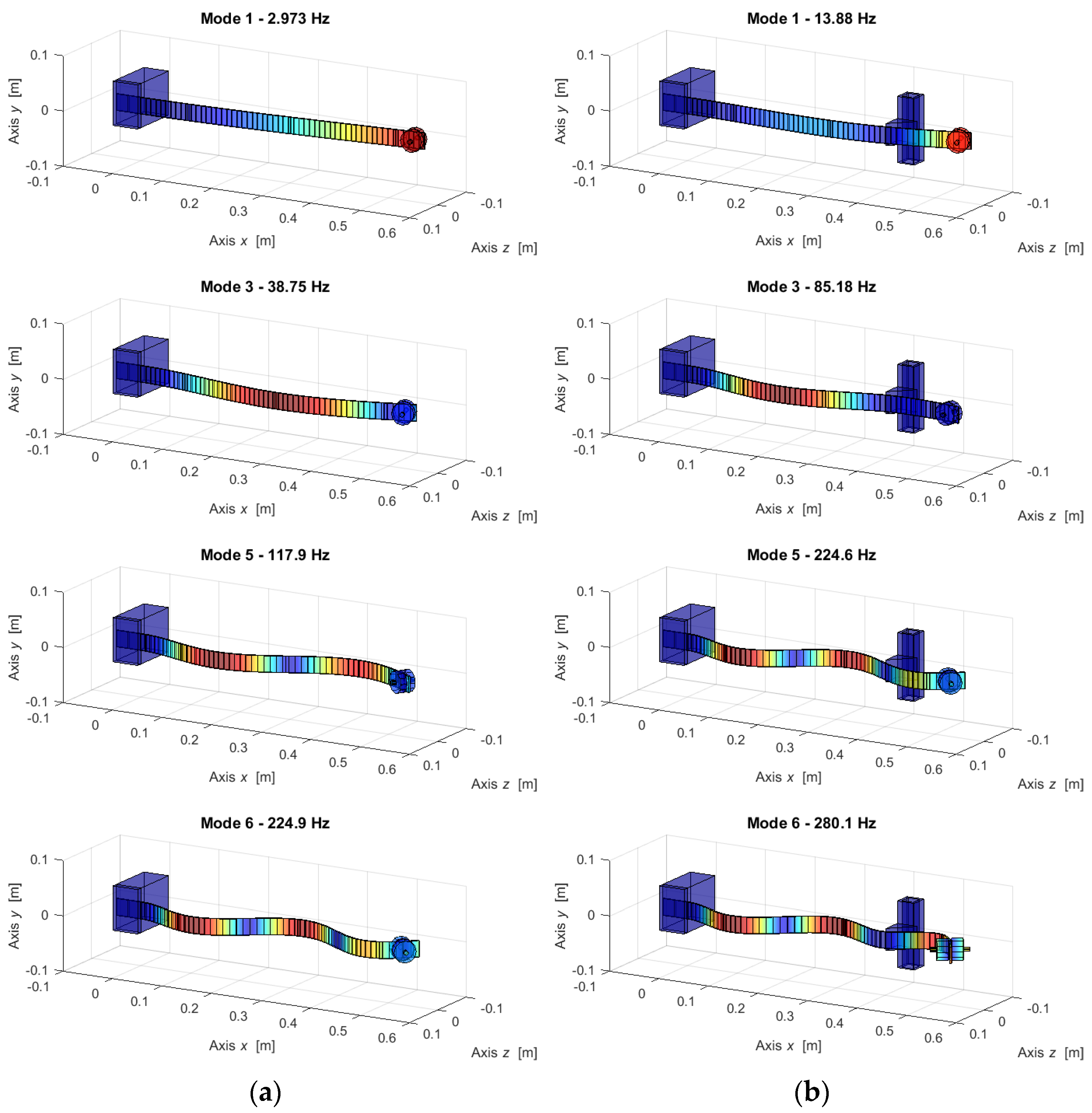
Figure 20 shows the two linearised configurations available in the CD test. The two configurations are modelled in the LUPOS environment.

Figure 20. LUPOS model for clamped-free beam (a) and clamped-pinned-free beam (b).

Figure 20. LUPOS model for clamped-free beam (a) and clamped-pinned-free beam (b).

Table 6. Results of modal analysis in the xz eigenspace.

Mode	Clamped-Free (Hz)	Clamped-Pinned-Free (Hz)	Description
1	2.973	13.88	First bending xz
2	38.75	85.18	Second bending xz
3	117.9	224.6	Third bending xz
4	224.9	280.1	Fourth bending xz

Table 6. Results of modal analysis in the xz eigenspace.

Mode	Clamped-Free (Hz)	Clamped-Pinned-Free (Hz)	Description
1	2.973	13.88	First bending xz
2	38.75	85.18	Second bending xz
3	117.9	224.6	Third bending xz
4	224.9	280.1	Fourth bending xz

In the clamped-free configuration, the beam nodes at the clamp have been locked imposing on the BCs for the six DoFs of each node, while the pinned configuration has been realised locking only the z displacement of the beam in correspondence with the non-symmetric constraint. The modal analysis in the two system configurations returns natural frequency values, which are collected in Table 6, only for the bending modes in xz plane.

The frequencies in Table 6 are now used to justify and proper interpret the graphs of the frequency contents of previous section, especially of experimental test CD in the 1st campaign. The natural frequency at 2.97 ÷ 3 Hz is visible in most of the figures displayed in the paper, and it is a validation of the experimental activity. The first four bending mode shapes in the xz plane for the two linearised systems are illustrated in Figure 21.

4. Conclusions

Results of the experimental campaign, carried out using Keyence laser profilometer LJ-X8900, have proven the feasibility of conducting high-frequency dynamic analyses with an instrument conventionally adopted in the production line for static detections of dimensions and tolerances in manufactured products.

The analyses were performed on experimental data measured in different setups, i.e., the common Euler–Bernoulli cantilever beam alone, the same subject to continuous nonlinearity of attractive or repulsive magnets, and, finally, the cantilever beam subject to non-holonomic contact.

The post-processing of the profilometer acquisitions show advantages and drawbacks in the exploited time–frequency analysis methods, which can be summarised in the following final remarks:

• The FFT allows to globally investigate the system behaviour, mainly concerning the fundamental frequencies and their superharmonics due to non-linearities, since the frequency resolution is defined, and it is maintained constant in the time–frequency analysis, from low to high frequencies. On the other hand, since the FFT frequency resolution is inversely proportional to the time resolution, an appropriate compromise between these two parameters is required. Consequently, the choice of a short time window that allows one to study fast-varying phenomena would result in a low frequency resolution that cannot properly allow one to obtain detailed frequency content information about the system;
• The CWT is used in addition to the latter, since the results of this approach demonstrate that it suits the analysis of dynamics characterised by almost instantaneous phenomena. The main drawback is a worsening of frequency resolution with the increment of frequency, in contrast with FFT analysis;
• FFT and CWT are both useful to study the same system from different perspectives and, together, allow to investigate both nonlinearities with their respective superharmonics and almost instantaneous phenomena.

The results achieved with the approaches above described are validated using the Hilbert transform to evaluate the instantaneous lowest frequency of the system, relating it with both time and displacement envelope. In addition to the described time–frequency analysis methods, two linear numerical models are developed to assess the experimental frequency overcomes, based on the averaged superposition of the natural frequencies of the two linear systems.

The correlation between the experimental data and the numerical data will be addressed in future research, based on Multi-Phi methodology, to investigate how nonlinear phenomena can be efficiently described by the convolution of linear systems effects.

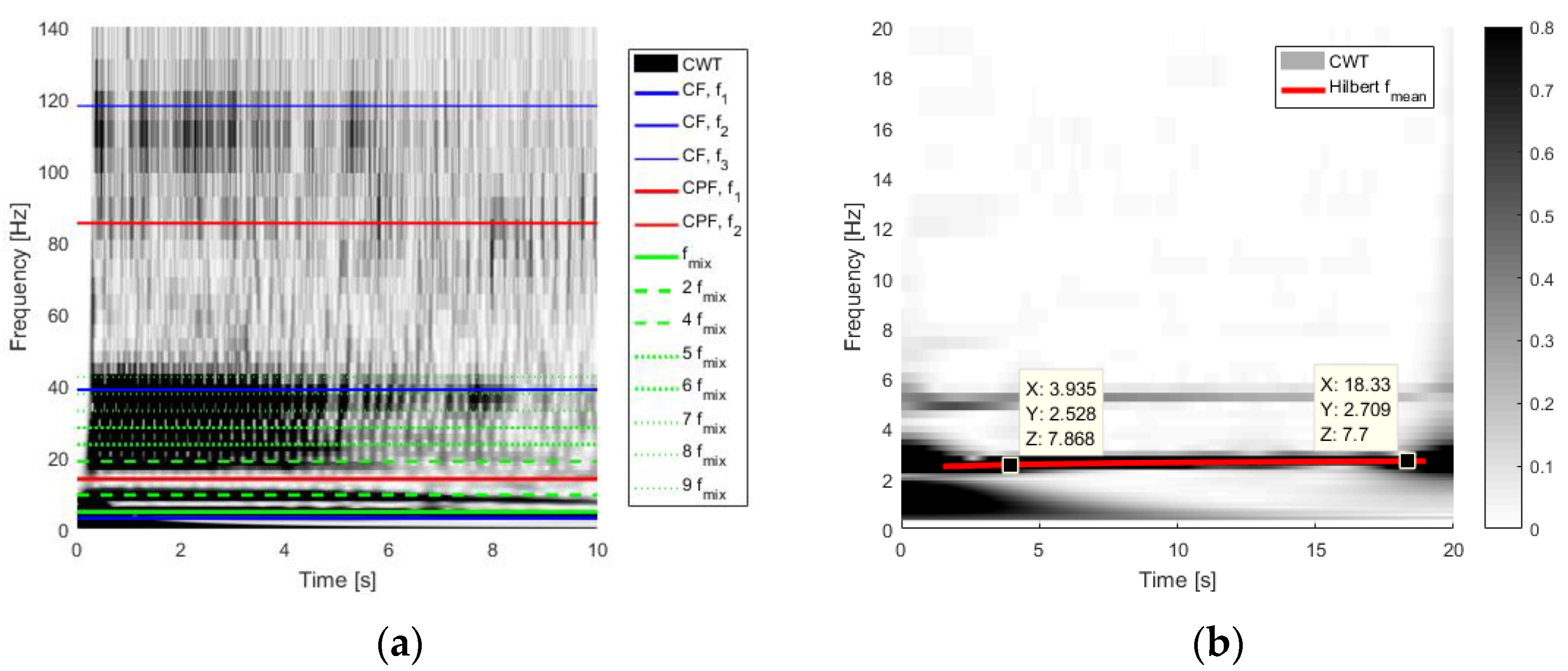
Finally, the correlation between the experimental data and the numerical ones in the case of attractive magnets is highlighted by Figure 22, which confirms the compliance between CWT method and Multi-Phi frequencies (a) and between the CWT approach and the Hilbert mean frequency (b), respectively. In Figure 22a, taking Table 6 into account, the blue lines correspond to the first three frequencies of the clamped free (CF) beam modes; the red lines to the first two ones of clamped pinned free (CPF) system modes; the continuous green line to the mixed frequency obtained as superposition of the first frequencies of CF and CPF systems, calculated in Equation (7); and the dashed green lines to the superharmonics of the latter. Figure 22b shows the correlation between the CWT time–frequency analysis and the mean frequency calculated with the Hilbert transform, instead.