Abstract
Understanding the many facets of repeated route choice behavior in traffic networks is essential for obtaining accurate flow forecasts and enhancing the effectiveness of traffic management measures. This paper presents a model of the day-to-day evolution of route choices incorporating travelers’ contrarian behavior, learning and inertia. The model is formulated as a discrete-time nonlinear dynamical system, and its properties are investigated analytically and numerically with a focus on the effect of the fraction of individuals adopting a contrarian route choice behavior. The findings of the study indicate that the extent of contrarian behavior may have significant impacts on the attractiveness and stability of network equilibria as well as on global system performance. We show that a properly balanced combination of direct and contrarian subjects can protect the system from instabilities triggered by other behavioral and network features. Our results also suggest that the fixed point stability range may depend to a considerable extent on travelers’ inertia and memory of previous experiences, as well as on the form of the travel cost functions used in the model. The occurrence of contrarian behavior should be explicitly taken into account in the design of traffic management schemes involving the deployment of Advanced Traveler Information Systems (ATISs), as it may act as a mitigating factor against the concentration of choices on the recommended routes. The analytical framework proposed in this paper represents a novel contribution, since contrarian behavior in repeated route choice has been investigated mainly by means of empirical or simulation approaches thus far.
1. Introduction
The behavioral mechanisms underlying the day-to-day evolution of route choices have been the object of active research within the field of transport analysis since the seminal work of Horowitz [1] demonstrated their impact upon the attractiveness and stability of equilibrium states in traffic networks. Understanding the fundamental drivers of day-to-day route choice behavior is of utmost importance for the prediction of users’ response to traffic management and information provision measures, notably the deployment of Advanced Traveler Information Systems (ATISs).
The study of day-to-day route choice dynamics in traffic networks can be undertaken either from a theoretical standpoint or through an empirical approach. With regard to discrete-time deterministic process models, which are of particular interest to our study, Cantarella and Cascetta [2] established general theoretical results, followed by several contributions dealing with specific aspects and applications [3,4,5,6,7].
Repeated route choice behavior has also been the object of empirical research, often focusing on the effects of experiential knowledge or ATIS-supplied information on the evolutionary dynamics of traffic networks. While virtual experiments in laboratory-like settings have been extensively used as a method of investigation [8,9,10,11,12,13,14,15], partially controlled on-road experiments [16,17] and analyses of large sets of route choice data observed in real networks have also been reported in the literature [18,19]. A connection between modeling and empirical approaches has been pursued as well [20,21,22].
The main purpose of the present study is to analyze how a specific feature, referred to as contrarian route choice behavior, may affect the day-to-day dynamics and the stability of traffic in transport networks. Generally speaking, contrarian behavior can be defined as a tendency to act “contrary to the crowd”, and can be observed in a variety of collective systems in which individual decisions are based on the expectation of the choices that are likely to be made by others. Contrarianism is thus a kind of strategic behavior that can be framed within the wider context of cognitive hierarchy theory [23]. The emergence of contrarian behavior has been addressed by studies relating to various fields, ranging from investment strategies in financial markets [24,25,26] to social psychology and opinion dynamics [27,28,29], and has been analyzed in the framework of game theory as well [30,31].
In order to introduce the setting of our study, we begin by presenting the basic concept through a simple example. Consider a group of travelers choosing repeatedly between two routes, denoted by 1 and 2, as in the case of individuals commuting daily from home to work. Route choices are dictated by expected travel times, say t1 and t2, which may be based on experiential knowledge and/or on navigational advice supplied by an ATIS. If, on any given day, t1 < t2, subjects choosing route 1 are said to exhibit direct choice behavior, while those selecting route 2 are said to exhibit contrarian choice behavior. The latter is inspired by strategic reasoning based on the presumption that the majority of travelers will behave in a direct manner. If this is indeed the case, route 1 is likely to become the more crowded, and thus contrarians may end up traveling on the fastest route. Clearly, contrarian behavior can be successful only as long as it is adopted by a minority of subjects within the traveling population.
Contrarian route choice behavior in traffic networks is a possible reaction of drivers to the information and recommendations supplied by route guidance systems [32], and has been investigated in several studies of day-to-day traffic dynamics adopting either experimental or agent-based simulation approaches. Selten et al. [9] found that contrarian behavior was adopted by a minority of the participants confronted with a two-route scenario in a laboratory experiment. Helbing et al. [33] introduced strategy coefficients in order to identify individual propensities toward direct or contrarian behavior in route choice games. In a controlled experiment on repeated route choice, Han et al. [34] detected the occurrence of strategic behavior, whereby some participants used ATIS recommendations as a means of anticipating other players’ decisions. Typical behaviors of participants in a two-route repeated choice experiment were classified using cluster analysis by Qi et al. [35], who studied the effect of providing full vs. partial travel time information on the fraction of contrarian responses. Meneguzzer [36] analyzed day-to-day route choices in a laboratory-like setting and found a prevalence of direct behavior, with contrarians achieving lower individual travel times than subjects who reacted in a direct manner to the provided information. As shown by an experimental study reported in [37], contrarian behavior may emerge not only under conditions of selfish routing, but also in a scenario of cooperative routing promoted by means of a system-optimal oriented ATIS.
Simulation-based studies have also addressed the issue of contrarianism in repeated route choice contexts. Bazzan et al. [38] proposed to model typical commuter route choice behaviors in a multi-agent system using the notion of personalities. They concluded that the best performing agents were subjects making choices that are opposite to those appearing as “good” on the basis of the recent outcomes. Alibabai and Mahmassani [39] applied the concept of strategic reasoning to simulate the day-to-day route choice behaviors of first-level and second-level thinkers in a simplified traffic system, and showed that strategic subjects could attain lower individual travel times only on the condition of being a minority within the population of network users.
Motivated by the lack of analytical (as opposed to experimental or simulation-based) studies of contrarianism in day-to-day route choice, Meneguzzer [40] proposed a macroscopic, closed-form model of traffic dynamics incorporating both direct and contrarian behaviors, and investigated several properties of the resulting nonlinear dynamical system.
The study described in the present paper extends and generalizes the above cited work of the author by:
- Introducing inertia into the dynamic process model representing the day-to-day evolution of the network state under mixed direct and contrarian route choices;
- Providing a more general statement of the fixed point stability conditions through the analysis of the Jacobian matrix of the resulting two-dimensional nonlinear dynamical system;
- Analyzing model behavior in the case of nonlinear link cost functions.
The remainder of the paper is organized as follows. In Section 2, the proposed model is formulated as a discrete-time nonlinear dynamical system, and the related analysis of fixed point stability is carried out. Section 3 illustrates the results of numerical tests of the model on a simple network under different assumptions about the form of the travel cost functions. The significance, limitations and policy implications of the research findings are discussed in Section 4, together with concluding remarks and suggestions for possible developments of the proposed approach.
2. Method
2.1. Model Formulation
We consider a two-link transportation network connecting a single Origin–Destination (O-D) pair and assume a total travel demand of 1 unit. Hence, the flow pattern is uniquely determined by the value of a single variable, and in the following analyses we denote by F the flow on link 1 and by (1 − F) the flow on link 2.
The day-to-day evolution of the network state is modeled by means of a discrete-time deterministic process whose generic period is denoted by t. Adopting a general approach which allows consideration of the effects of both memory and inertia upon the dynamics of travelers’ route choice behavior [2], the network dynamics can be described by the following recursive expressions:
where:
- (i = 1, 2) is the mean perceived cost of route i at the start of day t;
- (i = 1, 2) is the average flow-dependent cost actually experienced by users on route i;
- is the probability that a user who reconsiders their previous day’s choice will choose link 1 on day t, expressed as a function of the difference between day t’s perceived costs;
- () is a parameter quantifying the extent to which the most recent travel experience (“yesterday’s trip”) contributes to the formation of the cost perceived by users at the start of day t;
- () is a parameter representing the fraction of travelers who actually reconsider their previous day’s choice.
Expressions (1) and (2) provide a simplified but effective representation of the learning process by which network users develop their cost forecasts on the basis of past travel experiences. More specifically, can be interpreted as a memory depth parameter: in the limit, when travelers are “memoryless” as they base their next choice solely on the most recently experienced costs. Note that is excluded from the feasible range of the parameter because it would “freeze” the system’s dynamics by keeping mean perceived costs constant over time. On the other hand, expression (3) allows the incorporation of inertia and habitual behavior into the route choice process, as (1 − α) represents the fraction of users who repeat their previous day’s choice regardless of the cost actually experienced. In the limit, when inertia and habit effects are completely absent, while the value is excluded from the feasible range of the parameter because it would preempt the system’s dynamics by keeping flows constant over time.
Note that the unit of measurement of the travel cost variables appearing in Equations (1)–(3) and in all subsequent expressions is not specified because it does not affect the interpretation of the results nor the ensuing conclusions.
We now define and , and subtract expression (2) from expression (1) to obtain:
Substitution of expression (4) for into expression (5) yields the following two-dimensional nonlinear dynamical system:
whose fixed points correspond to states such that:
Using conditions (8) and (9), expressions (6) and (7) can be rewritten as:
or, equivalently:
and, substituting (12) for in expression (13), we obtain the following fixed point conditions:
Next, we address the specification of a route choice function S incorporating both direct and contrarian behaviors, as defined in the introductory remarks of Section 1. To this end, we propose a formulation encompassing the popular Logit model in its well-known conventional form (16) as a representation of direct choice behavior, and in a modified form, presented hereafter, as a representation of contrarian choice behavior. The two forms are then merged into a single model through a weighted combination reflecting the fractions of travelers adopting the two types of behavior. According to this approach, the probabilities of choosing route 1 are determined by means of expressions (16) and (17), respectively, for direct and for contrarian subjects:
where (>0) represents the dispersion parameter of the Logit model.
While the standard Logit model (16) is based on the assumption of cost-minimizing route choice behavior, expression (17) entails that the probability of a contrarian traveler choosing route 1 is an increasing function of the route’s expected cost. This is intended to model the propensity of contrarians to deliberately choose the route having higher expected cost, based on the belief that the majority of other travelers are likely to behave as cost minimizers. If this kind of strategic guess is correct, the route having the higher expected cost may turn out to be, after trips have been made, the less costly choice.
Letting denote the fraction of contrarian subjects within the traveling population (), we obtain the following expression for the probability of choosing route 1:
Introducing expression (18) into (7), the two-dimensional nonlinear dynamical system describing the day-to-day evolution of network states becomes:
and the fixed point conditions (14) and (15) can be rewritten as:
Note that the solution of the fixed point problem is independent of α and β, while, as shown in the following, these parameters play an important role in the context of the stability analysis of the dynamical system (19) and (20).
2.2. Fixed Point Stability Analysis
In order to analyze fixed point local stability, we consider the Jacobian matrix of system (6) and (7):
whose entries have the following expressions:
with:
According to a basic result of nonlinear dynamical systems theory, a fixed point is locally stable if the absolute values of all eigenvalues of matrix J evaluated at are less than 1. Expressions (29)–(31), often referred to as Jury conditions, are known to be necessary and sufficient for this:
where D is the determinant and T is the trace of matrix J evaluated at the fixed point:
Introducing (32) and (33) into conditions (29)–(31) yields:
It can be immediately seen that (34) always holds because and . In keeping with the main focus of this study, in what follows, we show how (35) and (36) can be converted into conditions on which define the range of values of the fraction of contrarian travelers ensuring fixed point stability.
To this end, we first evaluate the sign of . From the definition of :
it follows that:
under the natural assumption that the travel costs of both links are strictly increasing functions of the respective flows.
Since and , condition (35) requires:
Using expression (28), (39) can be written as:
from which the following condition on can be derived:
Next, we consider condition (36) and rewrite it as:
Using again expression (28) we obtain the following condition on :
Hence, we conclude that a fixed point is locally stable if:
with the lower and upper limits being effectively binding inside the range , that is for:
In light of the behavioral interpretation of parameters α and β provided in Section 2.1 we note that, in the particular case of a population of memoryless travelers (β = 1) completely free of inertia (α = 1), the range of values ensuring fixed point stability reduces to the following interval, which is symmetrical around :
subject to (46).
In the remainder of this subsection, we show how more specific fixed point stability results can be derived by assuming explicit forms of the link cost functions.
2.2.1. Fixed Point Stability in the Case of Linear Link Cost Functions
Let the travel cost functions of the two routes have the following forms:
where is a positive constant representing travel cost under free-flow conditions, and is a positive parameter representing the sensitivity of travel cost to flow. In spite of their simplified representation of traffic congestion, linear cost functions retain the essential property of being monotonically increasing with flow, and have been adopted in previous experimental studies on repeated route choices [9,14,15,35,41].
From (48) and (49) it follows that , so that (19) and (20) become:
and the fixed point conditions (21) and (22) can be rewritten as:
We can immediately see that is a solution to (52) and (53).
Since , the local stability condition (44) becomes:
with the lower and upper limits being effectively binding for:
Finally, in the particular case of a population of memoryless travelers (β = 1) completely free of inertia (α = 1), the range of values ensuring fixed point stability reduces to the following interval, which is symmetrical around :
subject to (56).
2.2.2. Fixed Point Stability in the Case of Fourth-Power Link Cost Functions
Assume now that the travel cost functions of the two routes have the following forms:
where and have the meaning already defined in Section 2.2.1. We note that (58) and (59) have the form of the classical BPR function, which is widely used in traffic assignment applications.
From (58) and (59) it follows that , so that system (19) and (20) becomes:
and the fixed point conditions (21) and (22) can be rewritten as:
Again, we can immediately see that is a solution to (62) and (63). Since in this case , the local stability condition (44) becomes:
with the lower and upper limits being effectively binding for:
Finally, in the particular case of a population of memoryless travelers (β = 1) completely free of inertia (α = 1), the range of values ensuring fixed point stability reduces to the following interval, which is symmetrical around :
subject to (66).
2.2.3. Discussion of Fixed Point Stability Results
The analytical results presented above, and notably conditions (54) and (64), suggest the following considerations:
- An adequately balanced mix of direct and contrarian subjects within the traveling population is conducive to fixed point stability, whereas strongly homogeneous route choice behaviors tend to trigger the occurrence of instabilities;
- The range of values ensuring fixed point stability depends on the inertia (α) and memory depth (β) parameters, as well as on the degree of sensitivity of costs to flows (γ) and of route choices to costs (μ);
- The stability regions defined by conditions (54) and (64) are not affected by a swap of the values of α and β or by a swap of the values of γ and μ;
- The width of the stability regions decreases as γ and/or μ increase. Unlike the latter parameters, which appear on both sides of expressions (54) and (64), α and β affect only the lower bound of the stability region. More specifically, it is easy to check that the derivatives of the left-hand sides of (54) and (64) with respect to α and β have a positive sign. In light of expressions (1)–(3), this suggests that appropriately reduced day-to-day cost and flow updating rates have the potential to offset the destabilizing effects of steeply increasing cost–flow functions and highly cost-sensitive route choice behaviors;
- Conditions (55), (56) and (65), (66) indicate that the composition of the traveling population in terms of direct/contrarian choice behaviors may become irrelevant when stability of the fixed point is already ensured by sufficiently small values of the other model parameters;
- Comparison of expressions (54) and (64) suggests that the stability region for fourth-power cost functions is twice as large as for linear cost functions. This circumstance can be explained by observing that, at the fixed point, the derivative of the fourth-power function is equal to , which is exactly half of the derivative of the linear cost function appearing in (54).
3. Numerical Examples
In order to provide a numerical and graphical illustration of the analytical results reported in the preceding section, we present here a few examples of the behavior of the proposed model under various combinations of system parameters. For the sake of brevity, all results are expressed in terms of only, since the addition of as a descriptor of the temporal evolution of the network state leads to qualitatively similar results. The cases of linear and fourth-power link cost functions are addressed separately in the next two subsections.
3.1. Linear Link Cost Functions
Table 1 shows the smallest (φ min) and largest (φ max) values of the fraction of contrarian travelers that ensure fixed point stability, computed by means of expression (54) for selected values of the other model parameters. Since , the lower limit of the stability region is set to zero whenever its calculated value turns out to be negative, and the upper limit is set to one whenever its calculated value exceeds unity.

Table 1.
Limits of the stability region in terms of φ for selected values of γμ, α and β in the case of linear link cost functions.
The results displayed in Table 1 provide numerical evidence in support of the conclusions ensuing from the preceding analytical study. In particular, when sensitivities of costs to flows and of route choices to costs are low (case γμ = 1), the fixed point turns out to be stable for any combination of direct and contrarian behaviors. As γμ grows, the stability region tends to shrink progressively; however, the increase of the lower stability limit (φ min) is offset by appropriately reduced day-to-day flow and cost updating rates, and therefore becomes apparent only for the higher values of α and β. Intuitively, this happens because travelers’ inertia and memory depth tend to act as damping forces against the destabilizing effects of high γ and μ values.
Examples of possible patterns of evolution of the network state over 100 time periods are presented in Figure 1 through 4 in order to illustrate the effects of the model parameters on the long-term outcome of the system’s dynamics. In these figures, t denotes the generic period (day) of the dynamic process and Z(t) represents the difference between the mean perceived costs of routes 1 and 2 at the start of day t, as defined in Section 2.1. While the trajectories shown in Figure 1 and Figure 2 are seen to converge to the fixed point (following either a smooth profile or a damped oscillatory pattern), in the case of Figure 3, the system is attracted to a period-2 cycle. A different kind of typical behavior emerges with the parameter values specified in Figure 4, where the network state converges without oscillations to an alternate fixed point unless initialized exactly at .
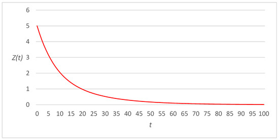
Figure 1.
Time evolution of dynamical system for (case of linear link cost functions).
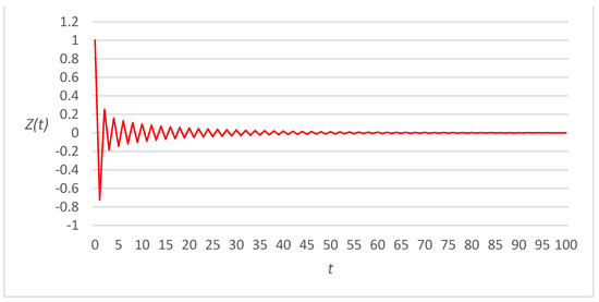
Figure 2.
Time evolution of dynamical system for (case of linear link cost functions).
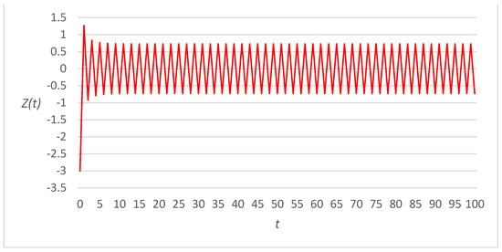
Figure 3.
Time evolution of dynamical system for (case of linear link cost functions).
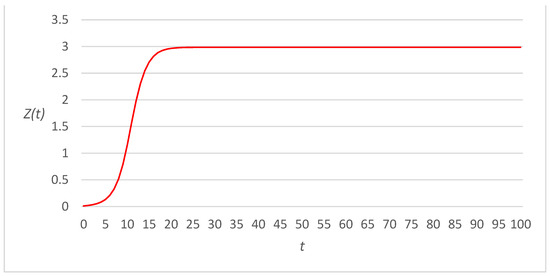
Figure 4.
Time evolution of dynamical system for (case of linear link cost functions).
The implications of contrarian route choice behavior for the performance of the network as a whole are illustrated in Figure 5 and Figure 6, which show the relationship between mean travel cost of all users and the fraction of contrarians for different values of and for two pairs of values of α and β. The results reported in these figures represent long-term states attained by the system after 1000 time periods, and were derived assuming in expressions (48) and (49). While Figure 5 refers to a population of users exhibiting a high level of inertia () and a deep memory of past travel costs (), Figure 6 addresses the case of highly reactive () and nearly memoryless () travelers. Both graphs clearly show that mean travel cost is lowest and remains constant over the region of stability of the fixed point, but increases steadily as moves outside this region. Comparison of the two figures further suggests that higher inertia and memory depth (Figure 5) tend to elongate this region leftwards by counteracting the instability which otherwise arises when contrarian subjects are underrepresented within the traveling population.
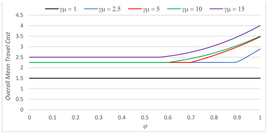
Figure 5.
Long-term overall mean travel cost as a function of for and different values of (case of linear link cost functions).
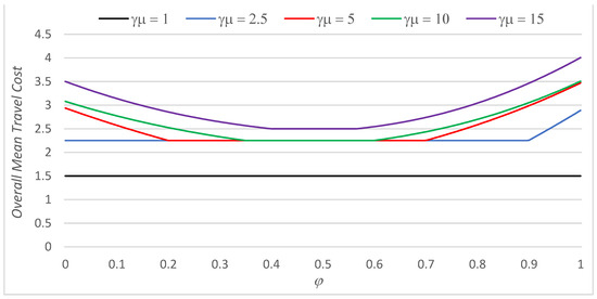
Figure 6.
Long-term overall mean travel cost as a function of for and different values of (case of linear link cost functions).
Figure 7 and Figure 8 provide evidence about the relative performance of the two types of travelers (as measured by the ratio of the respective mean travel costs) over the range of values of , having assigned to the other parameters the same values as in Figure 5 and Figure 6. The two subpopulations perform equally well over the region of stability of the fixed point, while an advantage associated with the minority route choice behavior emerges outside this range and tends to increase steadily as the size of the minority group decreases. This finding is consistent with the results reported in [31] based on a game-theoretical analysis. Comparison of the two figures indicates that a high level of inertia and a deep memory about past costs (Figure 7) have the potential to suppress the relative advantage of contrarian subjects when they represent a minority of the traveling population. A qualitatively similar effect in relation to travelers’ learning was found by Alibabai and Mahmassani [39] using a different approach.
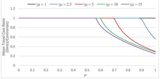
Figure 7.
Long-term ratio of direct to contrarian mean travel cost as a function of for and different values of (case of linear link cost functions).
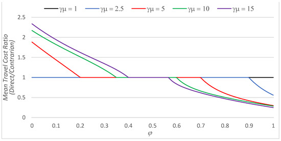
Figure 8.
Long-term ratio of direct to contrarian mean travel cost as a function of for and different values of (case of linear link cost functions).
3.2. Fourth-Power Link Cost Functions
Table 2 shows the smallest (φ min) and largest (φ max) values of the fraction of contrarian travelers that ensure fixed point stability, computed by means of expression (64) subject to , and assuming for the other model parameters the same values displayed in Table 1. As already explained in Section 2.2.3, the stability region for fourth-power cost functions is twice as large as for linear cost functions in all instances in which the calculated values of φ min and φ max fall inside the (0, 1) interval. Except for this difference, comparison of Table 1 and Table 2 suggests that the effects of parameters γμ, α and β are qualitatively similar in the two cases.
Table 2.
Limits of the stability region in terms of φ for selected values of γμ, α and β in the case of fourth-power link cost functions.
Examples of possible patterns of evolution of the network state over 100 time periods are presented in Figure 9, Figure 10, Figure 11 and Figure 12. In order to allow a meaningful comparison with the case of linear link cost functions, the values assigned to all parameters are equal to those used to derive Figure 1, Figure 2, Figure 3 and Figure 4. While the trajectories shown in Figure 9 and Figure 10 differ from those of Figure 1 and Figure 2 only for the faster convergence to the fixed point, Figure 11 suggests that with fourth-power cost functions the system is attracted to the fixed point rather than to a period-2 cycle, owing to the wider stability region. Last, comparison of Figure 4 and Figure 12 reveals that the network state converges to different non-zero fixed points in the two cases, as a consequence of the different assumptions about the form of the cost functions.
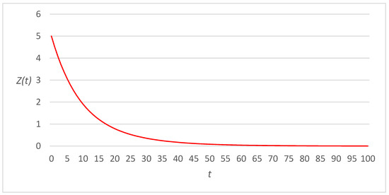
Figure 9.
Time evolution of dynamical system for (case of fourth-power link cost functions).
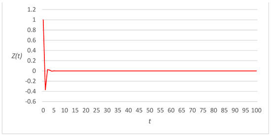
Figure 10.
Time evolution of dynamical system for (case of fourth-power link cost functions).
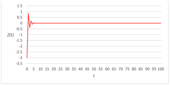
Figure 11.
Time evolution of dynamical system for (case of fourth-power link cost functions).
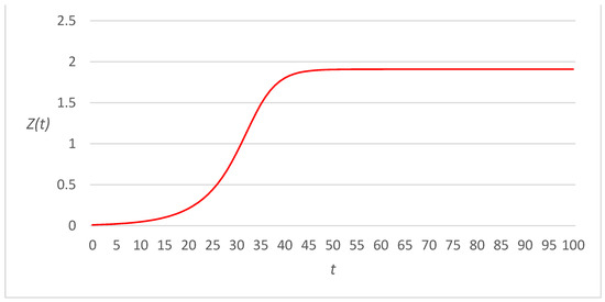
Figure 12.
Time evolution of dynamical system for (case of fourth-power link cost functions).
Finally, the results regarding overall mean travel cost and mean travel cost ratio obtained using fourth-power cost functions are qualitatively similar to those shown in Figure 5, Figure 6, Figure 7 and Figure 8, and lead to the considerations already presented in Section 3.1.
4. Discussion and Conclusions
The work reported in this paper provides an analytical framework for the study of contrarian behavior in repeated route choice situations, a topic that has been investigated mainly by means of empirical or simulation approaches thus far. Allowing a fraction of the network users to deliberately contradict the standard cost-minimizing route choice paradigm introduces into the modeling of day-to-day route choice a mix of behavioral attitudes which may have important implications for the long-term evolution of a traffic system.
The main policy implication of this study is that explicit consideration of the existence of contrarian behavior in route choices may enhance the accuracy of traffic flow forecasts, thus providing a better basis for the design and evaluation of traffic management strategies. As indicated by the analytical and numerical findings presented in this paper, contrarian behavior may have significant impacts on key properties of traffic systems, such as the attractiveness and stability of network equilibria, as well as on system performance metrics such as average travel time.
Another aspect of practical relevance of the study of contrarian route choice behavior relates in particular to the deployment of ATIS. The existence of individuals responding in a contrarian mode to the advice provided by these systems may act as a mitigating factor against the concentration of choices on the recommended routes, an adverse effect typically expected to occur as a result of ATIS deployment [42,43,44]. The ability of the traffic management agency to predict drivers’ reaction to information, taking into account the existence of contrarian responses, may result in improved forecasts, ultimately enhancing the credibility of the system.
Our findings clearly show that a balanced combination of direct and contrarian behaviors can protect the system from instabilities triggered by high sensitivities of travel costs to flows and of route choices to costs. This makes the results of our study particularly relevant to traffic systems characterized by significant levels of congestion and high ATIS market penetration, since under these circumstances an appropriate mix of direct and contrarian choice behaviors may become a key stabilizing factor. In addition, our results indicate that global network performance may benefit from a properly diversified composition of the traveling population in terms of direct and contrarian choice behaviors. Interestingly, these findings suggest that, from a traffic management standpoint, the fraction of travelers making contrarian route choices could be considered a control variable rather than a behavioral parameter. In practice, this could be achieved through properly designed policies for the allocation of personalized route recommendations in the context of ATIS [45], or through the definition of optimal routing strategies for connected and autonomous vehicles [46].
Inertia and memory of past travel experiences are important behavioral traits commonly found in real-world repeated route choice situations. Analysis of the effect of these characteristics in the proposed model suggests that they can counter the negative impact of low fractions of contrarian subjects on stability. This is due the smoothing effect induced by sufficiently small values of the parameters α and β in the flow and cost updating mechanisms, which reduces the rate of adjustment governing the underlying dynamical process. It follows that the case of inertia-free and memoryless travelers shown in Table 1 and Table 2, albeit unrealistic, provides an upper bound on the exposure of the system to the occurrence of instability. Although the determination of realistic values of the parameters representing inertia and memory depth is still an open question, experimental estimates of α and β are reported in a few studies on day-to-day route choice dynamics [12,36].
Another noteworthy result of the work described in this paper is that the choice of the specific form of the link cost functions should not be considered a marginal detail, as it may significantly affect the size of the fixed point stability region.
The findings of this study seem to support the conclusion that the potential impacts of contrarian behavior on the day-to-day dynamics of route choice are worthy of further in-depth investigation. The main limitation of this research relates to the simplicity of the network considered in the analysis, so that the principal aim of future research efforts should be the extension to general networks consisting of several origin–destination pairs connected by multiple routes. A key issue to be addressed in view of the implementation of the proposed model on real-world networks is the determination of empirically founded values of parameter . Estimating the extent to which contrarian behavior occurs in actual trip planning is surely a challenging task, that would require extensive collection of observations through controlled experiments or stated preference surveys. The “natural” target of such studies should consist of travelers actually experiencing repeated route choice situations, like individuals commuting daily from home to work.
Another simplifying assumption that needs to be removed in view of a generalization of the proposed model relates to the treatment of as an exogenously fixed parameter. In a realistic day-to-day route choice setting, the fraction of travelers adopting contrarian behavior is likely to be contingent upon the outcome of previous travel experiences, thus causing to become an endogenous, state-dependent parameter.
Funding
This research received no external funding.
Institutional Review Board Statement
Not applicable.
Informed Consent Statement
Not applicable.
Data Availability Statement
No data were used in this study.
Conflicts of Interest
The author declares no conflict of interest.
References
- Horowitz, J.L. The stability of stochastic equilibrium in a two-link transportation network. Transp. Res. B 1984, 18, 13–28. [Google Scholar] [CrossRef]
- Cantarella, G.E.; Cascetta, E. Dynamic processes and equilibrium in transportation networks: Towards a unifying theory. Transp. Sci. 1995, 29, 305–329. [Google Scholar] [CrossRef]
- Bie, J.; Lo, H.K. Stability and attraction domains of traffic equilibria in a day-to-day dynamical system formulation. Transp. Res. B 2010, 44, 90–107. [Google Scholar] [CrossRef]
- Meneguzzer, C. Dynamic process models of combined traffic assignment and control with different signal updating strategies. J. Adv. Transp. 2012, 46, 351–365. [Google Scholar] [CrossRef]
- Xiao, L.; Lo, H.K. Combined route choice and adaptive traffic control in a day-to-day dynamical system. Netw. Spat. Econ. 2015, 15, 697–717. [Google Scholar] [CrossRef]
- Xu, X.; Qu, K.; Chen, A.; Yang, C. A new day-to-day dynamic network vulnerability analysis approach with Weibit-based route adjustment process. Transp. Res. E 2021, 153, 102421. [Google Scholar] [CrossRef]
- Li, P.; Tian, L.; Xiao, F.; Zhu, H. Can day-to-day dynamic model be solved analytically? New insights on portraying equilibrium and accommodating autonomous vehicles. Transp. Res. B 2022, 166, 374–395. [Google Scholar] [CrossRef]
- Iida, Y.; Akiyama, T.; Uchida, T. Experimental analysis of dynamic route choice behavior. Transp. Res. B 1992, 26, 17–32. [Google Scholar] [CrossRef]
- Selten, R.; Chmura, T.; Pitz, T.; Kube, S.; Schreckenberg, M. Commuters route choice behavior. Games Econom. Behav. 2007, 58, 394–406. [Google Scholar] [CrossRef]
- Ben-Elia, E.; Shiftan, Y. Which road do I take? A learning-based model of route-choice behavior with real-time information. Transp. Res. A 2010, 44, 249–264. [Google Scholar] [CrossRef]
- Lu, X.; Gao, S.; Ben-Elia, E. Information impacts on route choice and learning behavior in a congested network: Experimental approach. Transp. Res. Rec. J. Transp. Res. Board 2011, 2243, 89–98. [Google Scholar] [CrossRef]
- Meneguzzer, C.; Olivieri, A. Day-to-day traffic dynamics: Laboratory-like experiment on route choice and route switching in a simple network with limited feedback information. Procedia Soc. Behav. Sci. 2013, 87, 44–59. [Google Scholar] [CrossRef]
- Rapoport, A.; Gisches, E.J.; Daniel, T.; Lindsey, R. Pre-trip information and route-choice decisions with stochastic travel conditions: Experiment. Transp. Res. B 2014, 68, 154–172. [Google Scholar] [CrossRef]
- Knorr, F.; Chmura, T.; Schreckenberg, M. Route choice in the presence of a toll road: The role of pre-trip information and learning. Transp. Res. F 2014, 27, 44–55. [Google Scholar] [CrossRef]
- Liu, S.; Guo, L.; Easa, S.M.; Yan, H.; Wei, H.; Tang, Y. Experimental study of day-to-day route-choice behavior: Evaluating the effect of ATIS market penetration. J. Adv. Transp. 2020, 2020, 8393724. [Google Scholar] [CrossRef]
- van Essen, M.; Thomas, T.; Chorus, C.; van Berkum, E. The effect of travel time information on day-to-day route choice behaviour: Evidence from a real-world experiment. Transp. B Transp. Dyn. 2019, 7, 1719–1742. [Google Scholar] [CrossRef]
- Wang, J.; Rakha, H. Empirical study of effect of dynamic travel time information on driver route choice behavior. Sensors 2020, 20, 3257. [Google Scholar] [CrossRef] [PubMed]
- Vacca, A.; Prato, C.G.; Meloni, I. Should I stay or should I go? Investigating route switching behavior form revealed preferences data. Transportation 2019, 46, 75–93. [Google Scholar] [CrossRef]
- Fusco, G.; Bracci, A.; Caligiuri, T.; Colombaroni, C.; Isaenko, N. Experimental analyses and clustering of travel choice behaviours by floating car big data in a large urban area. IET Intel. Transp. Syst. 2018, 12, 270–278. [Google Scholar] [CrossRef]
- Ye, H.; Xiao, F.; Yang, H. Exploration of day-to-day route choice models by a virtual experiment. Transp. Res. C 2018, 94, 220–235. [Google Scholar] [CrossRef]
- Li, W.; Ma, S.; Jia, N.; He, Z. An analyzable agent-based framework for modeling day-to-day route choice. Transp. A Transp. Sci. 2022, 18, 1517–1543. [Google Scholar] [CrossRef]
- Qi, H.; Jia, N.; Qu, X.; He, Z. Investigating day-to-day route choices based on multi-scenario laboratory experiments, Part I: Route-dependent attraction and its modeling. Transp. Res. A 2023, 167, 103553. [Google Scholar] [CrossRef]
- Camerer, C.F.; Ho, T.-H.; Chong, J.-K. A cognitive hierarchy model of games. Q. J. Econ. 2004, 119, 861–898. [Google Scholar] [CrossRef]
- Drehmann, M.; Oechssler, J.; Roider, A. Herding and contrarian behavior in financial markets: An internet experiment. Am. Econ. Rev. 2005, 95, 1403–1426. [Google Scholar] [CrossRef]
- Park, A.; Sgroi, D. Herding, contrarianism and delay in financial market trading. Euro. Econ. Rev. 2012, 56, 1020–1037. [Google Scholar] [CrossRef]
- Galariotis, E.C. Contrarian and momentum trading: A review of the literature. Rev. Behav. Financ. 2014, 6, 63–82. [Google Scholar] [CrossRef]
- Bagnoli, F.; Rechtman, R. Bifurcations in models of a society of reasonable contrarians and conformists. Phys. Rev. E 2015, 92, 042913. [Google Scholar] [CrossRef]
- Gambaro, J.P.; Crokidakis, N. The influence of contrarians in the dynamics of opinion formation. Physica A 2017, 486, 465–472. [Google Scholar] [CrossRef]
- Muslim, R.; Kholili, M.J.; Nugraha, A.R.T. Opinion dynamics involving contrarian and independence behaviors based on the Sznajd model with two-two and three-one agent interactions. Phys. D 2022, 439, 133379. [Google Scholar] [CrossRef]
- De Martino, A.; Giardina, I.; Marsili, M.; Tedeschi, A. Generalized minority games with adaptive trend-followers and contrarians. Phys. Rev. E 2004, 70, 025104. [Google Scholar] [CrossRef] [PubMed]
- Zhong, L.-X.; Zheng, D.-F.; Zheng, B.; Hui, P.M. Effects of contrarians in the minority game. Phys. Rev. E 2005, 72, 026134. [Google Scholar] [CrossRef] [PubMed]
- Bonsall, P. The influence of route guidance advice on route choice in urban networks. Transportation 1992, 19, 1–23. [Google Scholar] [CrossRef]
- Helbing, D.; Schönhof, M.; Stark, H.U.; Hołyst, J.A. How individuals learn to take turns: Emergence of alternating cooperation in a congestion game and the prisoner’s dilemma. Adv. Complex Syst. 2005, 8, 87–116. [Google Scholar] [CrossRef]
- Han, Q.; Timmermans, H.J.P.; Dellaert, B.G.C.; van Raaij, F. Route choice under uncertainty: Effects of recommendations. Transp. Res. Rec. J. Transp. Res. Board 2008, 2082, 72–80. [Google Scholar] [CrossRef]
- Qi, H.; Ma, S.; Jia, N.; Wang, G. Individual response modes to pre-trip information in congestible networks: Laboratory experiment. Transp. A Transp. Sci. 2019, 15, 376–395. [Google Scholar] [CrossRef]
- Meneguzzer, C. Contrarians do better: Testing participants’ response to information in a simulated day-to-day route choice experiment. Travel Behav. Soc. 2019, 15, 146–156. [Google Scholar] [CrossRef]
- Klein, I.; Ben-Elia, E. Emergence of cooperative route-choice: A model and experiment of compliance with system-optimal ATIS. Transp. Res. F 2018, 59, 348–364. [Google Scholar] [CrossRef]
- Bazzan, A.L.C.; Bordini, R.H.; Andrioti, G.K.; Vicari, R.M.; Wahle, J. Wayward agents in a commuting scenario (personalities in the minority game). In Proceedings of the Fourth International Conference on Multi Agent Systems, Boston, MA, USA, 10–12 July 2000. [Google Scholar]
- Alibabai, H.; Mahmassani, H.S. Foxes and sheep: Effect of predictive logic in day-to-day dynamics of route choice behavior. EURO J. Transp. Logist. 2016, 5, 53–67. [Google Scholar] [CrossRef]
- Meneguzzer, C. Day-to-day dynamics in a simple traffic network with mixed direct and contrarian route choice behaviors. Phys. A 2022, 603, 127841. [Google Scholar] [CrossRef]
- Wang, S.-Y.; Guo, R.-Y.; Huang, H.-J. Day-to-day route choice in networks with different sets for choice: Experimental results. Transp. B Transp. Dyn. 2021, 9, 712–745. [Google Scholar] [CrossRef]
- Ben-Akiva, M.; de Palma, A.; Kaysi, I. Dynamic network models and driver information systems. Transp. Res. A 1991, 25, 251–266. [Google Scholar] [CrossRef]
- Wahle, J.; Bazzan, A.L.C.; Klugl, F.; Schreckenberg, M. The impact of real-time information in a two-route scenario using agent-based simulation. Transp. Res. C 2002, 10, 399–417. [Google Scholar] [CrossRef]
- Ben-Elia, E.; Avineri, E. Response to travel information: A behavioural review. Transp. Rev. 2015, 35, 352–377. [Google Scholar] [CrossRef]
- Klein, I.; Levy, N.; Ben-Elia, E. An agent-based model of the emergence of cooperation and a fair and stable system optimum using ATIS on a simple road network. Transp. Res. C 2018, 86, 183–201. [Google Scholar] [CrossRef]
- Mansourianfar, M.H.; Gu, Z.; Waller, S.T.; Saberi, M. Joint routing and pricing control in congested mixed autonomy networks. Transp. Res. C 2021, 131, 103338. [Google Scholar] [CrossRef]


Disclaimer/Publisher’s Note: The statements, opinions and data contained in all publications are solely those of the individual author(s) and contributor(s) and not of MDPI and/or the editor(s). MDPI and/or the editor(s) disclaim responsibility for any injury to people or property resulting from any ideas, methods, instructions or products referred to in the content. |
© 2023 by the author. Licensee MDPI, Basel, Switzerland. This article is an open access article distributed under the terms and conditions of the Creative Commons Attribution (CC BY) license (https://creativecommons.org/licenses/by/4.0/).