Automatic Decentralized Vibration Control System Based on Collaborative Stand-Alone Smart Dampers

Abstract

In many structures, undesired noise and vibrations generated by external sources represent a huge problem in terms of structural damage and comfort. Active vibration absorbers can be used to dynamically suppress vibrations, by increasing the damping of the system. A wireless smart active damper has been developed to perform this task and some automated functionalities have been implemented to perform the identification of the structure on which it is mounted on. The sharing of information between wireless sensors represents one of the most interesting features of this kind of control system. In this work, a procedure to estimate the nondimensional damping and modal amplitude for each wireless sensor location and each vibration mode is studied. Then, the information obtained by each sensor in the identification phase are used to implement a coordinated control strategy, which is based on a modified version of the Efficient Modal Control (EMC). Such control strategy implements the low level Selective Negative Derivative Feedback control law and modulates the control gains of each actuator and controlled mode pair in order to get an effective vibration reduction. The tuning procedure represents the next step of the algorithm, in which the evaluation of the introduced damping and the maximum applicable gains are derived; finally, the proposed solution is validated with experimental results on a simply-supported beam.

1. Introduction

Active vibration control (AVC) by means of electrodynamic proof-mass actuators (PMA) represents a valid alternative to traditional passive tuned mass dampers [1] in order to suppress vibrations. In AVC, the advantage is represented by the possibility to introduce damping on more than one vibration mode. To do so, proof-mass actuators (PMA) are widely used, due to their easy mounting since they do not need to react off the base structure [2,3,4]. Therefore, the number of PMA on a structure can be easily increased and then the capability of the overall system to introduced damping increases.

For all these reasons, a control system based on PMA has been developed in [5], where vibration suppression on a large structure was required. The PMA prototype is driven by a printed circuit board (PCB). In the PCB, an accelerometer samples the structure acceleration providing the feedback signal. This signal is used by the microcontroller for the computation of the control action, which is amplified by an analog conditioning circuit and fed into the actuator. These embedded features allows the PMA to work autonomously, thus no centralized regulator is necessary. For this reasons, such actuators are also named “Stand-alone smart dampers”. Moreover, one of the most interesting feature of the device is the wireless module integrated on the PCB. This allows information and data sharing between the smart dampers. To date, the development of wireless solutions is ongoing also in other fields, like the vibration monitoring of cargo trains and the wind-induced vibrations of HVTL conductors [6,7,8,9].

This wireless data sharing between devices has been already used in a control system, where two wireless nodes were considered [10,11]. A Selective Negative Derivative Feedback (SNDF) control law has been implemented in [10]. Such control law filters out the local acceleration measurement by means of a band-pass filter centered on the considered eigenfrequency. The filtered acceleration is then integrated and multiplied by a control gain in order to compute the control force. The SNDF makes the system more robust to spillover and instability phenomenon related to the low frequency PMA phase shift. Compared to the Direct Velocity Feedback (DVF) control law, SNDF provides higher control gains and then more damping can be introduced. Some different solutions have already been studied to solve the instability problems of PMA [12], but the SNDF represents one of the most reliable one. Some automated functionalities have been developed in order to allow the control system to recognize the structure on which is mounted on. Each wireless sensor can recognize the natural frequencies of the hosting structure and the actual vibration conditions and share the results with the other devices. The final target is to develop a smart control system able to extract as many information as possible from the structure and automatically tune the control action according to the information obtained. The information sharing between wireless nodes is used to get a global overview of the hosting structure and to define a coordinated control strategy.

In this work, starting from the described system, some functionalities have been developed. In particular, a procedure to estimate the non-dimensional damping and modal amplitude for each wireless sensor location and each vibration mode is proposed. The information obtained by the structure and vibration identification phase are exploited to implement a coordinated control strategy, based on a modified version of the Efficient Modal Control (EMC) proposed by [13]. Such control strategy is based on the low level SNDF control law and modulates the control gains of each actuator-controlled mode pair in order to get an effective vibration reduction. The control gains are weighted according to the excitation state of the hosting structure and to the performance of the each actuator to introduce damping in each mode. The latter weighting feature represents the novelty with respect the traditional EMC.

The paper is structures as follows. In Section 2 the structure identification phase is described according to the developed functionalities, focusing on the estimation of the damping ratio and the structural gain. In Section 3 the coordinated control strategy based is presented. In Section 4 the mathematical derivation of the formulas used to calculate the maximum gain which ensure the stability of the closed−loop system and the maximum saturation gain are derived. In Section 5 are reported the numerical and experimental results. Finally, conclusions are drawn in Section 6.

2. Modal Parameters Identification

The aim of this project is the development of an adaptive control system which can automatically modify the control policy. In this way, the stand-alone devices can be installed on whatever structure and actively control vibrations without any a priori knowledge on its dynamics.

In the first step, the natural frequencies of the structure must be detected. The superimposition of coupled modes may affect the results of the modal identification, although such phenomena usually occur in the high frequency range. In this work, the controlled modes are sufficiently unrelated to be clearly identified. So, each actuator is used as a disturbance source, in order to excite the structure in a given range of frequencies. During the sweep excitation of an actuator, the collocated sensor acquires the acceleration signal in order to get the spectrum and then find out the eigenfrequencies. One by one, each stand-alone device perform this task, since the position of the device on the structure may affect the results. Once these operations are over, the information collected by the stand-alone devices are shared with the Central Control Unit (CCU). Such operations have been already implemented and described in [10].

The second phase is related to the evaluation of the non-dimensional damping ratio ${\xi }_{i,j}$ and the structural gain $R_{i,j}$. Each actuator performs its own evalutions of ${\xi }_{i,j}$ and $R_{i,j}$, for the i-th vibration mode and the j-th actuator. The two parameters play a central role for the setting of the band-pass filter and of the control gains, as reported in Section 4.

2.1. Non-Dimensional Damping Ratio Evaluation

Among the several techniques used to evaluate the non-dimensional damping ratio, a time domain decrement method has been chosen, to limit the computational effort. A time domain method allows a faster identification since all the measures needed for the computation of the modal parameters (the damping ratio ${\xi }_i$ and the structural gain $R_{i,j}$) can be recorded through just one harmonic excitation of the structure for each mode. The time domain decrement method relies on the assumption that the primary structure can be modeled as a single DOF system. During modal parameter estimation, just one mode at the time is excited by one actuator and no disturbance forces are supposed to excite the structure. Moreover, such hypothesis is verified only if a given vibration mode is not affected by the others.

As for the sweep, the CCU sends the command to the stand-alone devices to start the modal parameter identification procedure. One by one, each actuator excites one by one all the modes. The actuator applies a constant amplitude harmonic force, whose frequency matches the desired mode natural frequency. As soon as the excitation gets a steady-state condition, the acceleration of the primary structure and the acceleration of the proof-mass are recorded (the proof-mass acceleration signal is available through another digital accelerometer, which is placed on the proof-mass and directly connected to the PCB). Then, the harmonic excitation stops and the device acquires the vibration decay of the excited mode. An algorithm will chose one peak at the beginning ($u_1$) and one at the end ($u_2$) of the vibration decay. The parameter $u_1$ is always chosen as the second peak of the vibration decay (the reason of this choice will be give afterwards in Section 5.3.1). The parameter $u_2$, instead, is the first peak whose amplitude is less then the $20\%$ of $u_1$. Once this harmonic excitation has been carried out for any i-th observable vibration mode, the non-dimensional damping ratio ${\xi }_{i,j}$ is evaluated for any vibration mode as:

$${\xi }_{i,j}=\frac{\Delta u}{2\pi n{u}_m}$$

(1)

where $\Delta u=u_1-u_2$, $u_m=\frac{u_1+u_2}{2}$ and n is the number of periods considered between the two peaks.

2.2. Structural Gain Evaluation

In order to evaluate the structural gain, the ratio between the maximum of primary structure acceleration ${\ddot{y}}_{max,i,j}$ and proof-mass acceleration ${\ddot{x}}_{max,i,j}$ is computed for each i-th mode and each j-th actuator. Starting from the transfer function between the acceleration measured at the actuator location $\ddot{Y}\left(s\right)$ and the transmitted force $F_T\left(s\right)$, defined in the Laplace domain:

$$\frac{\ddot{Y}\left(s\right)}{F_T\left(s\right)}=R_{i,j}\frac{s^2}{s^2+2{\xi }_i{\omega }_{i}s+{\omega }_i^2}$$

(2)

we can substitute $F_T\left(s\right)=-m_a\ddot{X}\left(s\right)$ and $s=j\omega$ in Equation (2) as follows:

$$\frac{\ddot{Y}\left(j{\omega }_i\right)}{\ddot{X}\left(j{\omega }_i\right)}=-j\frac{m_a{R}_{i,j}}{2{\xi }_i}$$

(3)

This means that only the imaginary part of the FRF is considered. However, in the algorithm applied on the microcontroller, the solution is approximated by taking the ratio of the two maximum values of the acceleration (${\ddot{y}}_{max,i,j}$ and ${\ddot{x}}_{max,i,j}$) rather than the imaginary part of the FRF. This approximation simplifies a the computational effort, since it is not necessary the computation of the FFT. This assumption is also justified by the steady-state condition of the signals and leads to the final definition of the structural gain:

$$R_{i,j}=\frac{2{\xi }_i}{m_a}\frac{{\ddot{y}}_{max,i,j}}{{\ddot{x}}_{max,i,j}}$$

(4)

3. Coordinated Control Strategy

In some cases, a significant reduction on vibrations is required, then a common solution is to place many actuators on the structure. In this way, more damping can be introduced in the system, as described in [14]. For this reason, in this work, three actuators have been used.

Now, it is necessary to develop an automatic algorithm for the computation of the control gain for each actuator. Such an algorithm will be designed according to the coupling between each actuator and the controlled modes. The Efficient Modal Control (EMC) proposed in [13] represents a suitable solution for this purpose. In the EMC, a proper gain is assigned to any controlled mode in order to get a control action generated by each actuator which is coordinated with the others. In this way, the control action of each device will be focused only on the controllable modes, in particular on the ones related to the larger vibration amplitudes.

In the first step of the algorithm, the additional modal damping that can be introduced by each actuator is evaluated. Then, the EMC will be explained and the modified version of such strategy will be presented.

3.1. Introduced Active Damping Ratio

In the EMC strategy, the introduced non-dimensional damping is used for the modulation of the control action. In this section, the mathematical expression of the damping introduced by an actuator into a generic vibration mode is derived.

Taking into account the SNDF control law defined in [10] and assuming the i-th vibration mode excited (the module of the band-pass compensator corresponding to the compensator frequency is 0 $\left[dB\right]$), the dissipated energy related to the electromagnetic force of the actuator $F_a=BlI$ evaluated within an oscillation period is:

$$E_{d,F_a}={\int }_0^T{B}_a{l}_a{g}_{i,j}^{\mathrm{*}}{\dot{y}}^{2}dt={\int }_0^T{g}_{i,j}{\dot{y}}^{2}dt$$

(5)

where $\dot{y}$ is the structure velocity and $g_{i,j}^{\mathrm{*}}$ is the control gain. The current absorbed by the actuator is $I=g_{i,j}^{\mathrm{*}}\dot{y}$.

Now, the dissipated energy can be expressed in terms of modal coordinates. Considering an harmonic disturbing force $Q_{i}cos\left({\omega }_{i}t\right)$ which affect the structure, whose frequency is the same of the structure i-th eigenfrequency, the formulation of the dissipated energy becomes:

$$E_{d,F_a,i}=\pi g_{i,j}{\varphi }_{i,j}^2{Q}_i^2{\omega }_i$$

(6)

where ${\varphi }_{i,j}$ is the modal amplitude. Then, the non-dimensional damping ratio can be defined as a function of $E_{d,F_a,i}$:

$$h_{i,j}=\frac{E_{d,i}}{2\pi m_i{Q}_i^2{\omega }_i^2}=\frac{E_{d,i}}{4\pi E_{k,i}}$$

(7)

where $E_{k,i}$ is the maximum kinetic energy related to the i-th vibration mode. Finally, by substituting Equation (6) into Equation (7):

$$h_{i,j}=\frac{g_{i,j}{\varphi }_{i,j}^2}{2m_i{\omega }_i}=\frac{g_{i,j}{R}_{i,j}}{2{\omega }_i}$$

(8)

As shown in Equation (8), the introduced damping ratio $h_{i,j}$ depends also on the control gain $g_{i,j}$ applied on the i-th mode, which should be considered as a known parameter. Since the aim is to increase as much as possible the damping introduced, the gain must be the highest possible. However, the maximum feasible gain is limited by instability or saturation phenomena which affect the PMA. As a result, the gain $g_{i,j}$ in Equation (8) is the minimum between the maximum gain which ensure the stability of the closed−loop system (related to the actuator dynamics) and the saturation one. The derivation of these limiting gains will be presented in Section 4.

3.2. Modified Efficient Modal Control

The introduced active damping ratio defined in the previous section represents a key parameter for the derivation of the control law. In case of several devices placed on the same structure, it is possible to compare and rank the actuators according to the damping introduced by each one.

The next step is the definition of a procedure to evaluate the optimal gain for each stand-alone device of the control system, as a function of the controlled modes. In the EMC, a relative weight between the control gains is introduced, which allows to reduce the degrees of freedom of the problem. Therefore, only the absolute magnitude of this gains has to be evaluated, in order to avoid instability or saturation phenomena of the actuator, as mentioned before.

The EMC strategy represents a valid alternative to the centralized solutions like the so-called Independent Modal Space Control (IMSC) and Modified IMSC (MIMSC), since allows to decrease the amplitude of vibration in a minimum period of time, thus limiting the control effort. In this strategy the gains applied for each mode are weighted according to the modal vibration displacement or to the modal energy.

In this work, a modified version of the EMC is proposed. The aim is to provide a control law with a simpler implementation, by limiting as much as possible the time for on-line computing. In the EMC, the gains are defined through an optimization algorithm which is unfeasible in this case, due to the the limited performance of the microcontroller. Then, the goal is to merge the information related to the introduced damping found before and the amplitude of vibration associated to each mode. Therefore, the maximum gain will be multiplied by two weights which are related to the modal vibration displacement and the introduce damping. In the following, the definition of these weights is presented.

3.2.1. Modal Displacement Weight

The modal displacement (or vibration amplitude) weight $w_{Y,i,j}$ has already been used in [13] and it is defined as the ratio between the vibration amplitude $Y_{i,j}$ and the maximum vibration amplitude $Y_{max}$:

$$w_{Y_{i,j}}=\frac{Y_{i,j}}{Y_{max}}$$

(9)

where $Y_{i,j}$ is the displacement amplitude observed by the j-th actuator for the i-th mode and $Y_{max}=max\left(Y_{i,j}\right)$. These vibration amplitudes can be evaluated at the vibration state analysis stage, when the FFT of the uncontrolled system is computed. Notice that the PCB measures the acceleration of the structure, thus the information obtained by the FFT is the acceleration amplitude ${\ddot{Y}}_{i,j}$. Hence, being ${\ddot{Y}}_{i,j}=Y_{i,j}{\omega }_i^2$, the definition of the vibration amplitude weight as to be changed into:

$$w_{Y_{i,j}}=\frac{{\ddot{Y}}_{i,j}}{{\ddot{Y}}_{max}}·\frac{{\omega }_{Y_{max}}^2}{{\omega }_i^2}$$

(10)

where ${\ddot{Y}}_{max}=max\left(\frac{{\ddot{Y}}_{i,j}}{{\omega }_i^2}\right)$ and ${\omega }_{Y_{max}}$ is the natural frequency of the mode with the maximum amplitude displacement. Notice that this weight tends to be higher for the low frequency modes. Indeed, usually, the displacements are related to such modes.

3.2.2. Introduced Damping Weight

The novelty of this method with respect to EMC is to exploit the introduced damping as a weighting parameter. The introduced damping weight is calculated in Equation (11) as the ratio of the damping, introduced by the j-th actuator in the i-th mode, and the maximum damping introduced among any actuator-mode couple:

$$w_{h_{i,j}}=\frac{h_{i,j}}{h_{max}}$$

(11)

where $h_{i,j}$ is calculated through Equation (8) and $h_{max}=max\left(h_{i,j}\right)$.

3.2.3. Gain Modulation

The maximum applicable gains must be modulated as follows:

$$g_{i,j}=w_{h_{i,j}}·w_{Y_{i,j}}·g_{max,i,j}·\gamma$$

(12)

where $w_{h_{i,j}}$ and $w_{Y_{i,j}}$ are the introduce damping and displacement weights respectively. The parameter $g_{max,i,j}$ is the maximum gain which can be applied to avoid saturation and instability phenomena.

This consideration is only valid if the j-th actuator just works on the i-th mode and neither other modes are controlled nor other actuators work. As described before, the EMC allows to reduce the number of DOF related to the gains setting. The only parameter which must be defined is $\gamma$. The parameter $\gamma$ has the same value for all $g_{i,j}$. This additional multiplication is necessary since the overall combination of gain could lead the system to instability, as shown in [15,16]. In this case, $\gamma$ is initially set to 1 and it must be reduced till stability is reached or if some actuator saturates. The evaluation of the overall degree of saturation $S_j$ is provided by the sum of each degree of saturation $S_{i,j}$ related to each controlled mode. The derivation of the degree of saturation will be carried out in the next sections.

4. Limitations on the Control Gain

The definition of the control gains represents one of the main aspects of this work, since in this way the control system can adapt the control law to any situation in an automated way. For example, if the nature of the disturbance changes during time, the control system will tune the control gains in a different way.

The use of inertial actuator implies a restriction on the maximum feasible gain. This limitation has been highlighted in many works [15,17,18] and an evaluation of the maximum gain related to the actuator dynamics for the Direct Velocity Feedback (DVF) control law has been presented in [19]. However, the limitation on the control gain is affected not only from instability phenomena, but also from stroke and current saturations. As described in the previous sections, the maximum feasible gain $g_{i,j}$ which can be set by the actuator is the minimum between the maximum gain related to the actuator dynamics and the saturation one.

In this work, the problem of instability has been addressed from a more general point of view. The effect of the actuator dynamics has been studied not only on the controlled mode, but also on the others. For both cases, it was demonstrated a way to evaluate the maximum gain related to the actuator dynamics, when a SNDF control logic is used. At this stage, the assumption is that just one PMA works on a given mode to be controlled. Moreover, a mathematical expression to calculate the maximum gain that prevents the actuator saturations is derived.

4.1. Actuator Dynamics Effect

The problem of instability generated by the coupling between the proof-mass actuator and the hosting structure can be addressed by considering the complete controlled system in Laplace domain. A flexible structure can be modeled as a single DOF system, under the assumption that there is only one mode excited and controlled.

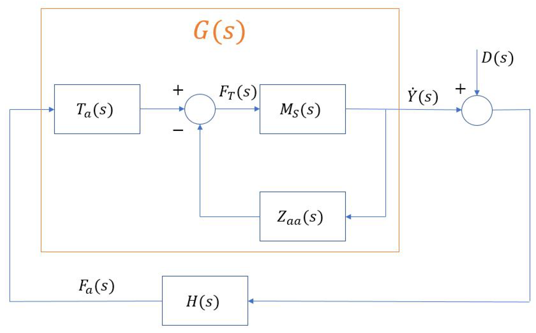
For this reason, to simplify the discussion, the system is supposed to be a Single Input Single Output (SISO) system, where the input is the electromagnetic force $F_a\left(s\right)$ and the output is the structure response due to the controlled vibration mode $\dot{Y}\left(s\right)$. Into the block diagram in Figure 1, which represents the overall control system [20], the mobility transfer function $M_s\left(s\right)$, the blocked response transfer function $T_a\left(s\right)$ and the actuator mechanical impedance $Z_{aa}\left(s\right)$ are defined as follows ($m_a$, $c_a$ and $k_a$ are the mass, damping and stiffness of the actuator respectively):

$$\begin{array}{cc}\hfill M_s\left(s\right)& =\frac{\dot{Y}\left(s\right)}{F_T\left(s\right)}=R_{i,j}\frac{s}{s^2+2{\xi }_i{\omega }_{i}s+{\omega }_i^2}\hfill \\ \hfill T_a\left(s\right)& =\frac{F_T\left(s\right)}{F_a\left(s\right)}=\frac{m_a{s}^2}{m_a{s}^2+c_{a}s+k_a}\hfill \\ \hfill Z_{aa}\left(s\right)& =\frac{F_T\left(s\right)}{\dot{Y}\left(s\right)}=\frac{m_a(c_{a}s+k_a)s}{(m_a{s}^2+c_{a}s+k_a)}\dot{Y}\left(s\right)\hfill \end{array}$$

(13)

we can derive the plant transfer function $G\left(s\right)$ of the controlled system:

$$G\left(s\right)=\frac{m_a{R}_{i,j}{s}^3}{(s^2+2{\xi }_i{\omega }_{i}s+{\omega }_i^2)(m_a{s}^2+c_{a}s+k_a)+m_a{R}_{i,j}(c_{a}s+k_a)s^2}$$

(14)

and we can reduce the whole model to the canonical form containing the controller transfer function $H\left(s\right)$ and the plant $G\left(s\right)$, as shown in Figure 1.

In $H\left(s\right)$, expressed in Equation (15), we have applied the SNDF control logic, where we have centered the band-pass filter on the i-th vibration mode eigenfrequency (i.e. ${\omega }_c={\omega }_i$) and considered ${\xi }_c={\xi }_i$.

$$H\left(s\right)=-\frac{g_i(2{\xi }_c{\omega }_c+d_c)s}{s^2+(2{\xi }_c{\omega }_c+d_c)s+{\omega }_c^2}$$

(15)

Hence, the open−loop transfer function can be easily defined and can be written in a simple way by grouping the same order denominators terms:

$$GH\left(s\right)=\frac{g_i(2{\xi }_c{\omega }_c+d_c)m_a{R}_{i,j}{s}^4}{B_6{s}^6+B_5{s}^5+B_4{s}^4+B_3{s}^3+B_2{s}^2+B_{1}s+B_0}$$

(16)

where:

$$\begin{array}{cc}\hfill B_6& =A_4\hfill \\ \hfill B_5& =A_3+(2{\xi }_c{\omega }_c+d_c)A_4\hfill \\ \hfill B_4& =A_2+(2{\xi }_c{\omega }_c+d_c)A_3+{\omega }_c^2{A}_4\hfill \\ \hfill B_3& =A_1+(2{\xi }_c{\omega }_c+d_c)A_2+{\omega }_c^2{A}_3\hfill \\ \hfill B_2& =A_0+(2{\xi }_c{\omega }_c+d_c)A_1+{\omega }_c^2{A}_2\hfill \\ \hfill B_1& =(2{\xi }_c{\omega }_c+d_c)A_0+{\omega }_c^2{A}_1\hfill \\ \hfill B_0& ={\omega }_c^2{A}_0\hfill \\ \hfill A_4& =m_a\hfill \\ \hfill A_3& =c_a+2{\xi }_i{\omega }_i{m}_a+m_a{R}_{i,j}{c}_a\hfill \\ \hfill A_2& =k_a+2{\xi }_i{\omega }_i{c}_a+m_a{R}_{i,j}{k}_a+{\omega }_i^2{m}_a\hfill \\ \hfill A_1& =2{\xi }_i{\omega }_i{k}_a+{\omega }_i^2{c}_a\hfill \\ \hfill A_0& ={\omega }_i^2{k}_a\hfill \end{array}$$

(17)

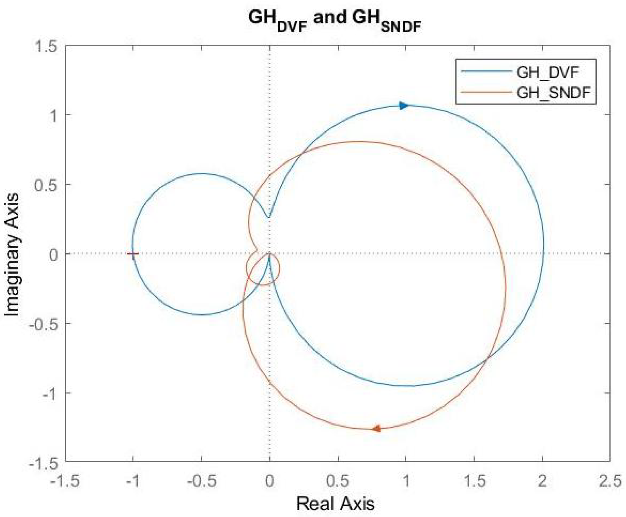
Looking at the Nyquist plot in Figure 2 obtained by Equation (16), there is an encirclement as in the case of the DVF, where $H\left(s\right)=g$. The presence of this encirclement is due to the resonance of the proof-mass actuator and affects the system stability. In this case, the same gain has been applied on both control laws, ensuring the stability of the SNDF as opposed to the DVF.

In order to define the maximum gain related to the actuator dynamics, Equation (16) is rewritten by substituing $s=j\omega$ and by splitting the real part from the imaginary one. The numerator, with the imaginary part equal to zero, can be written as:

$$G{H}_{num}\left(j\omega \right)=g_i(2{\xi }_c{\omega }_c+d_c)m_a{R}_{i,j}{\omega }^4=R_N\left(j\omega \right)$$

(18)

while the denominator becomes:

$$G{H}_{den}\left(j\omega \right)=\underset{{\displaystyle R_D\left(j\omega \right)}}{\underbrace{-B_6{\omega }^6+B_4{\omega }^4-B_2{\omega }^2+B_0}}+j\underset{{\displaystyle I_D\left(j\omega \right)}}{\underbrace{(B_5{\omega }^5-B_3{\omega }^3+B_1\omega )}}$$

(19)

Now, the maximum gain related to the actuator dynamics $g^{\mathrm{*}}$ must be defined. First of all, by imposing $I_D\left({\omega }^{\mathrm{*}}\right)=0$ the frequency ${\omega }^{\mathrm{*}}$ is:

$${\omega }^{\mathrm{*}}=\sqrt{z_2}=\sqrt{\frac{B_3-\sqrt{{B_3}^2-4B_5{B}_1}}{2B_5}}$$

(20)

Then, since ${\omega }^{\mathrm{*}}$ is known, the gain $g^{\mathrm{*}}$ is obtained by imposing the real part of the open−loop transfer function $GH(j{\omega }^{\mathrm{*}},g^{\mathrm{*}})$ equal to −1:

$$g^{\mathrm{*}}=\frac{B_6{\omega }^{\mathrm{*}6}-B_4{\omega }^{\mathrm{*}4}+B_2{\omega }^{\mathrm{*}2}-B_0}{m_a{R}_{i,A}(2{\xi }_c{\omega }_c+d_c){\omega }^{\mathrm{*}4}}$$

(21)

In Equation (21) it is shown that the computation of such gains depends on several parameters. In particular, the maximum gain related to the actuator dynamics depends mainly on the ratio between the mode natural frequency and the actuator natural frequency $\raisebox{1ex}{${\displaystyle {\omega }_i}$}\!\left/ \!\raisebox{-1ex}{${\displaystyle {\omega }_a}$}\right.$ and on the structural gain $R_{i,j}$. If the control mode has a frequency close to the actuator one, then the maximum gain related to the actuator dynamics results very low, as shown in [19].

4.2. Stroke Saturation

A significant limiting factor on the maximum feasible gain concerns the actuator saturation. An inertial actuator can saturate in two ways, depending on the frequency of the vibration mode. If the mode frequency is lower than the saturation break frequency of the actuator (${\omega }_{sat,break}=\sqrt{\frac{F_{a,max}}{m_{a}d}}$, where $F_{a,max}$ is the maximum electromagnetic force that the actuator can exert, $m_a$ is the proof-mass and d is the maximum stroke), then stroke saturation will occur, otherwise current saturation arises, as explained in [21]. The two phenomena are different, thus they require a specific saturation definition.

Starting from the stroke saturation and assuming the i-th mode of the primary structure to be excited, the stroke saturation required to control the i-th vibration mode can be defined as:

$$S_{i,d}=\frac{|x_{F_A}+x_{{\dot{y}}_i}|}{d}$$

(22)

where $x_{F_A}$ is the vibrating mass displacement due to electromagnetic force, $x_{{\dot{y}}_i}$ is the one due to the velocity of the structure and d is the maximum stroke allowed. Then, Equation (22) can be expressed in terms of current and gain as follows:

$$\begin{array}{cc}\hfill S_{i,d}& =\frac{1}{d}\left|\frac{B_a{l}_a}{-{\omega }_i^2{m}_a+j{\omega }_i{c}_a+k_a}{I}_i+\frac{j{\omega }_i{c}_a+k_a}{j{\omega }_i(-{\omega }_i^2{m}_a+j{\omega }_i{c}_a+k_a)}{\dot{y}}_i\right|\hfill \\ \hfill & =\frac{1}{d}\left|\frac{g_i}{j{\omega }_i(-{\omega }_i^2{m}_a+j{\omega }_i{c}_a+k_a)}+\frac{j{\omega }_i{c}_a+k_a}{-{\omega }_i^2(-{\omega }_i^2{m}_a+j{\omega }_i{c}_a+k_a)}\right|\left|{\ddot{y}}_i\right|\hfill \end{array}$$

(23)

The only term of the band-pass filter still included into the equation is $g_i$, since the compensator transfer function [10] evaluated on the resonance is equal to 1. However, the filtering effect of the compensator introduce the assumption that the acceleration measured by the actuator is just related to the i-th mode. For this reason, the notation of the acceleration $\ddot{\left|y\right|}$ becomes $\left|{\ddot{y}}_i\right|$. By splitting again the imaginary and the real part of the expression into the absolute value operator:

$$S_{i,d}d=\left|\frac{j(EB+GA)+EA-GB}{A^2+B^2}\right|\left|{\ddot{y}}_i\right|$$

(24)

where:

$$\begin{array}{cc}\hfill A& =m_a{\omega }_i^5-k{\omega }_i^3\hfill \\ \hfill B& =c_a{\omega }_i^4\hfill \\ \hfill D& =c_a{\omega }_i^2\hfill \\ \hfill E& =k_a{\omega }_i\hfill \\ \hfill G& =g_i{\omega }_i^2+D\hfill \end{array}$$

(25)

Since the aim is to calculate the maximum gain, we impose $S_{i,d}=1$ and then we can solve Equation (24) with respect to G (which depends on $g_i$):

$$g_{i,stroke}=\frac{\sqrt{\frac{d^2\left[{\left(m_a{\omega }_i^5-k_a{\omega }_i^3\right)}^2+{\left(c_a{\omega }_i^4\right)}^2\right]}{{max\left(\left|{\ddot{y}}_i\left(j{\omega }_i\right)\right|\right)}^2}-k_a^2{\omega }_i^2}-c_a{\omega }_i^2}{{\omega }_i^2}$$

(26)

4.3. Current Saturation

A similar procedure like the one proposed for the stroke saturation can be used to calculate the maximum gain that leads to the current saturation. First of all, the saturation rate related to the control action on the i-th vibration mode is defined as a function of the control gain:

$$S_{i,I}=\frac{\left|I_{max,i}\right|}{I_{max}}=\frac{g_i\left|\ddot{\frac{y_i}{j{\omega }_i}}\right|}{I_{max}}$$

(27)

By solving the equation with respect to $g_i$ and imposing $S_{i,I}=1$ (as well as in the previous equation):

$$g_{i,current}^{\mathrm{*}}={\omega }_i\frac{I_{max}}{max\left(\left|{\ddot{y}}_i\right|\right)}⟶g_{i,current}=Bl{g}_{i,current}^{\mathrm{*}}$$

(28)

where B and l are the magnetic flux density and the length of the coil of the actuator respectively. For both stroke and current saturation, the maximum gain depends on the modulus of the acceleration related to the i-th mode ${\ddot{y}}_i$. This parameter can be evaluated in the vibration analysis phase, where FFT operations have been performed by all wireless sensors to get the vibration state of the structure.

5. Results

5.1. Test Bench Arrangement

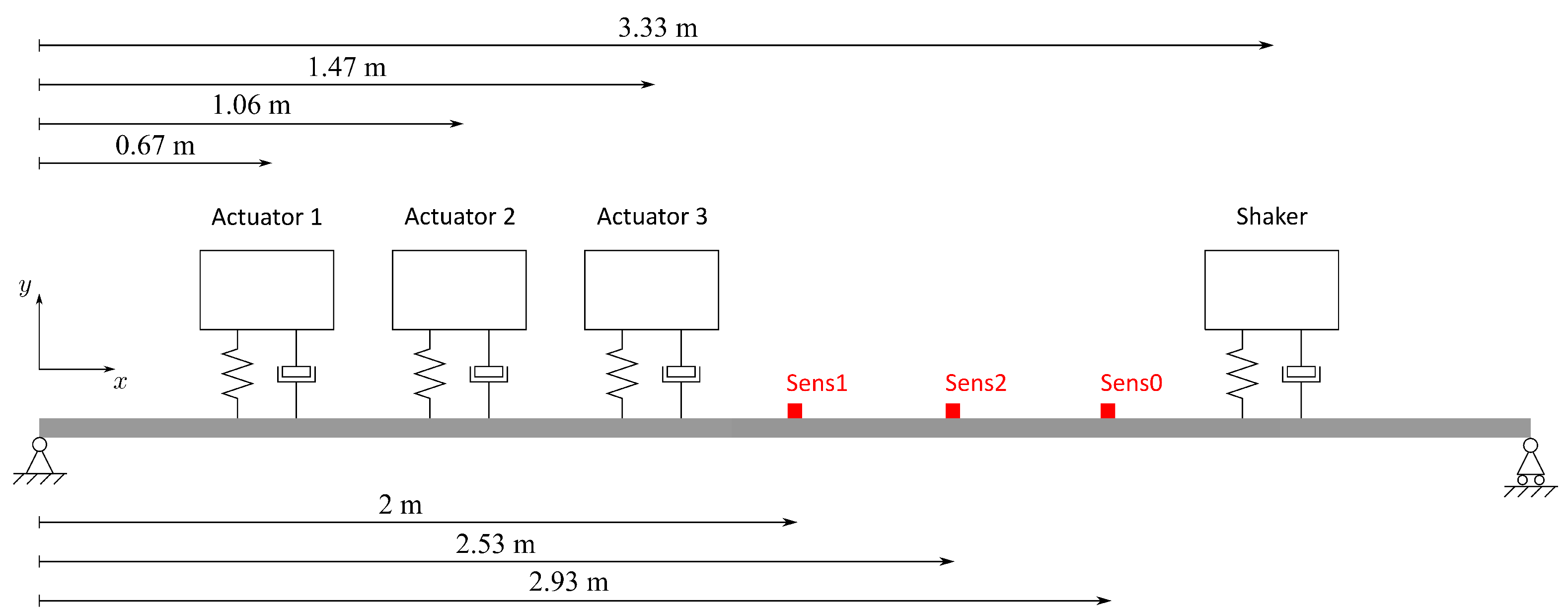
In this section, a description of the experimental test bench is reported. The host structure is a double-T profile beam (IPE120), which is simply supported at its ends (Figure 3a). Its geometrical and physical parameters are reported in

Table 1. Beam parameters.

Parameters	Length	Section Area	Linear Mass	Inertia Moment	Young Modulus
IPE120	4 [m]	13.2 [cm${}^2$]	10.4 [$\frac{\mathrm{Kg}}{\mathrm{m}}$]	318 [cm${}^4$]	206 [GPa]

.

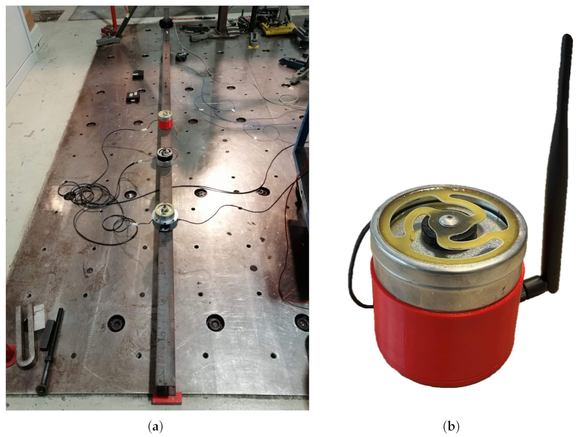
Three proof-mass actuators (Figure 3b) are placed on the beam according to the scheme depicted in Figure 4 (a detailed description of the modeling process of the actuator is reported in [5]). The position of the actuators has been chosen according to three anti-nodal points of the beam. Actuator 1 is placed on an anti-node of the third vibration mode of the beam, while Actuator 2 and 3 respectively on the anti-nodes of the second and fourth mode of the beam. Since the first vibration mode has a frequency lower than the actuators one, it cannot be controlled (due to the actuators dynamics). Due to the co-located control (sensor and actuator are embedded on the same device), the performance of the control system will depend on the position of the smart dampers on the structure. So, a correct installation of such devices is required. Three additional accelerometers are placed on the second-half of the beam with the same principle, in order to externally measure the performance of the control system. Sensor 0 is placed on the anti-node of the second mode and sensor 1 and 2 on the anti-nodes of the third and fourth mode respectively. In

Table 2. Comparison between the natural frequencies of the considered modes (numerical and experimental).

	Mode 2	Mode 3	Mode 4
$f_{num}$ [$\mathrm{Hz}$]	91.2	202.6	331.8
$f_{exp}$ [$\mathrm{Hz}$]	90.3	204.5	335.1

the natural frequencies of the selected modes are reported, both for numerical simulations and experimental tests. The disturbance force is generated by another electrodynamic PMA placed on the structure. In this case, its position has been chosen properly in order to excite the second, third and fourth mode of the beam at the same time.

5.2. Numerical Results

At the beginning, the proposed EMC strategy has been tested by means of numerical simulations. In this way, the performance of this control strategy has been verified.

The starting point for this analysis is the calculation of the final control gains, as shown in Equation (12). The limiting gain between the maximum gain related to the actuator dynamics and saturation gains is the one related to the current saturation, which is assigned to the parameter $g_{max,i,j}$. Then, the introduced damping and modal displacement weights are calculated according to Equations (10) and (11), considering a given vibration state. Finally, the multiplication between the two weights provide the final weight that modulates $g_{max,i,j}$.

The final step regards the tuning of $\gamma$. As a first trial, $\gamma$ has been set equal to 1. The saturation degree has been computed for each the three actuators as follows:

$$S_j=\sum _{i=2}^4{g}_{i,j}\frac{{\ddot{y}}_{i,j}}{{\omega }_i}\frac{1}{F_{a,j,max}}$$

(29)

where ${\ddot{y}}_{i,j}$ is the modulus of the acceleration related to the i-th mode measured by the j-th actuator and $F_{a,j,max}$ is the maximum electromagnetic force that the j-th actuator can apply.

The results showed that the saturation condition was not satisfied for actuator 2, since $S_2>1$. This is due to the final weight $w_{2,2}$ equal to 1. Since the gain $g_{max,2,2}$ is already the maximum saturation gain to control only mode 2, if actuator 2 is required to control also mode 3 and 4, the saturation degree $S_2$ overcomes the threshold of $100\%$. For this reason, the value of $\gamma$ must be lower than 0.985. Then, the overall combination of gains has been tested considering the control enabled on each actuator. This procedure is necessary to assess the stability of the overall system, otherwise a further reduction of $\gamma$ is requested.

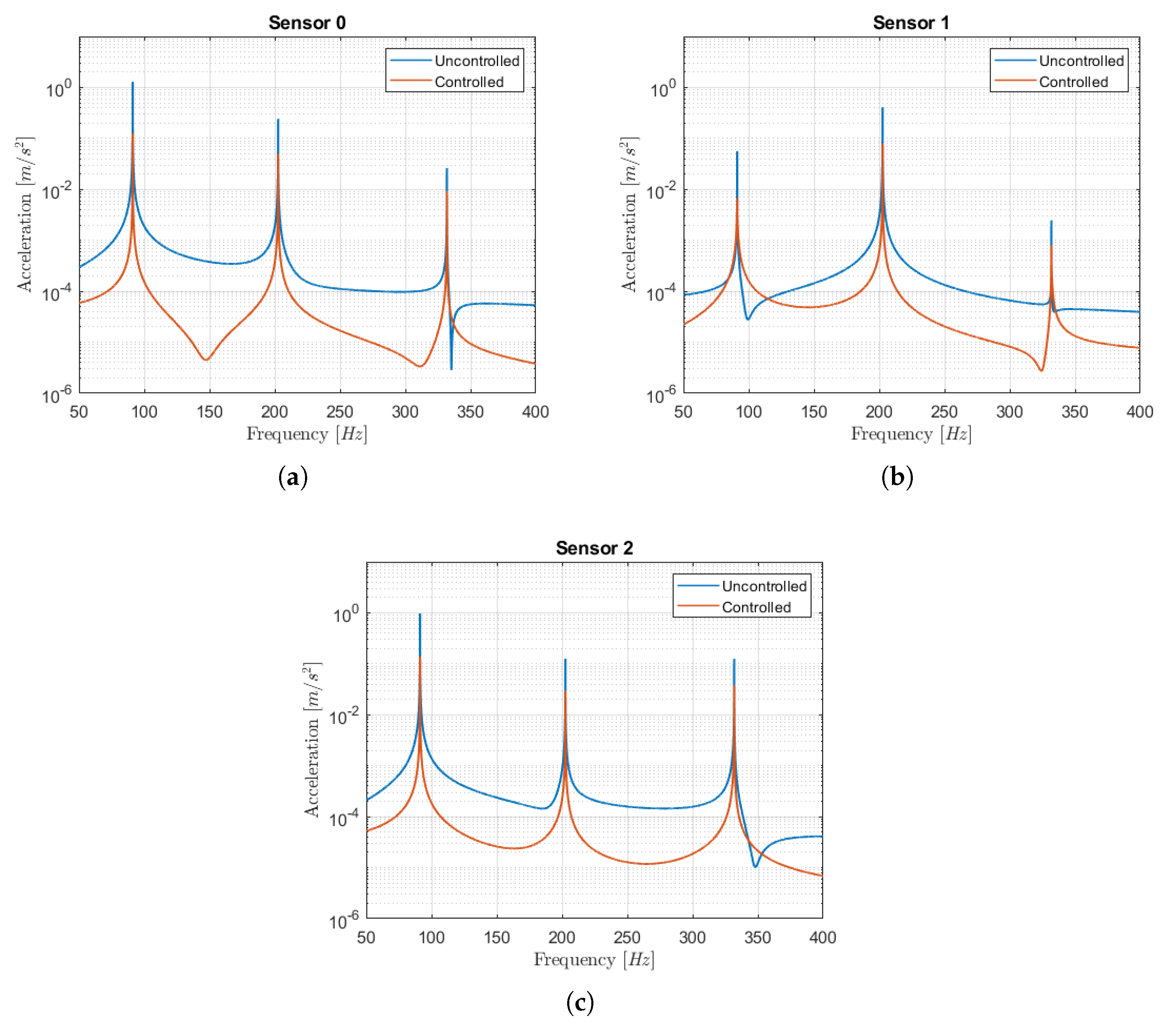
The results obtained on the controlled system are compared with the uncontrolled one, as shown in

Table 3. Vibration comparison between uncontrolled and controlled case in numerical simulation.

	Mode	Sensor 0	Sensor 1	Sensor 2
Uncontrolled [$\mathrm{m} {\mathrm{s}}^{-2}$]	2	1.3050	0.0559	0.9734
	3	0.2424	0.4100	0.1268
	4	0.0264	0.0021	0.1251
Controlled [$\mathrm{m} {\mathrm{s}}^{-2}$]	2	0.1263	0.0067	0.1396
	3	0.0505	0.0800	0.0298
	4	0.0093	0.0008	0.0378
Reduction [%]	2	90.32	88.10	85.66
	3	79.17	80.49	76.48
	4	64.79	63.04	69.82

. In Figure 5 are depicted the FRFs in the sensors positions (Sensor 0, 1 and 2 as reported in Figure 4), both for the uncontrolled and the controlled case. Looking at the results, on the mode 2 (where most of the damping power is focused) the largest reduction is obtained, which is about $90\%$ on the vibration amplitude. About modes 3 and 4, a reduction about $78\%$ and $65\%$ is achieved.

5.3. Experimental Results

The proposed methods for the evaluation of the damping ratio ${\xi }_{i,j}$ and structural gain $R_{i,j}$ have been tested experimentally. In order to verify the accuracy of the obtained results for the damping ratio estimation, a preliminary analysis is required. So, the damping ratios of all the considered modes have evaluated by means of the Half-power method and the Hilbert transformation method. Then, the results obtained can be compared with the decay method.

5.3.1. Non-Dimensional Damping

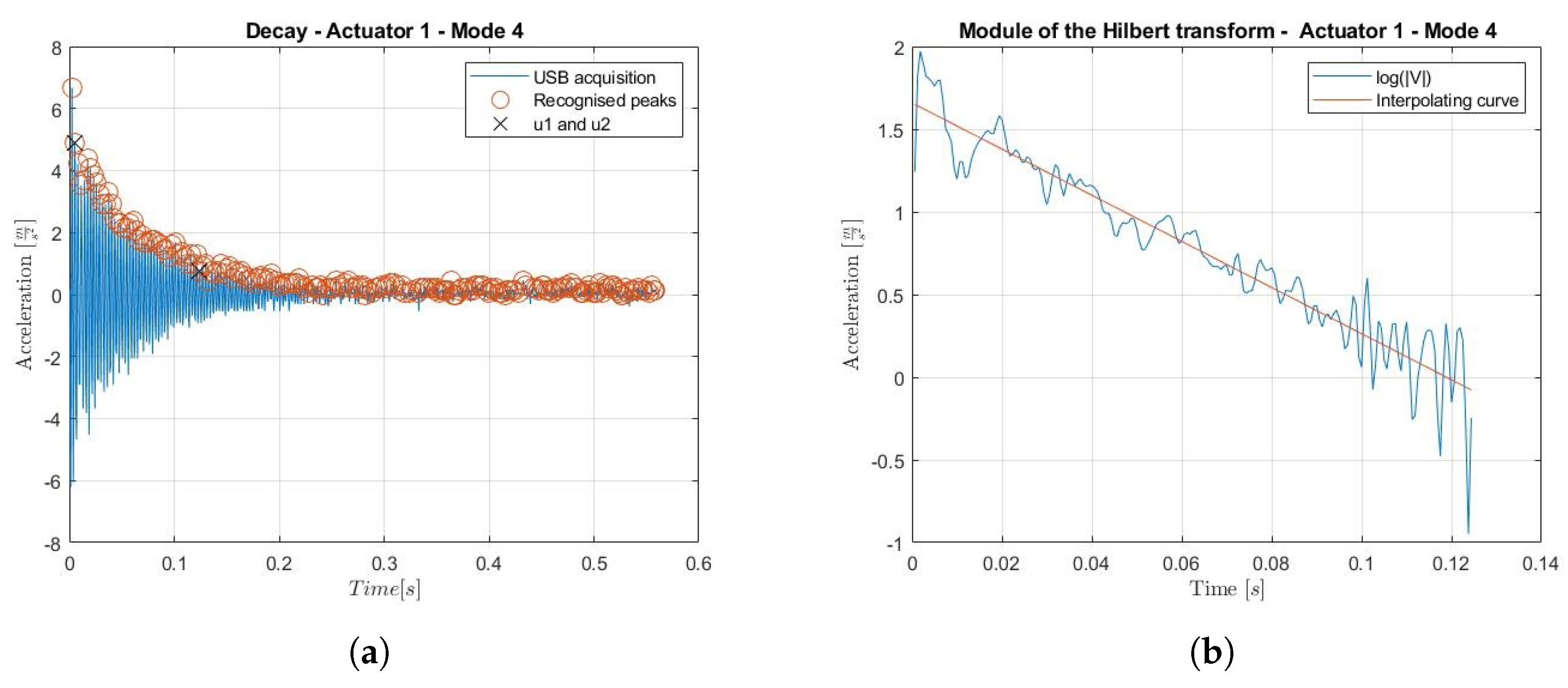
The decay method proposed in Section 2.1 has been tested for all the three actuators. As an example, only the results related ot Actuator 1 are reported, which are shown in

Table 4. Estimation of the damping ratio ${\xi }_{i,j}$ for the Actuator 1 compared with Hilbert transform and Half-power methods.

Mode	Decay Method	Hilbert tr. Method	Half-Power Method	Error w.r.t. Hilbert tr. m. [%]	Error w.r.t. Half-Power m. [%]
2	0.0125	0.0146	0.0321	14.3	61.1
3	0.0035	0.0036	0.0042	2.2	17.3
4	0.0057	0.0063	0.0102	9.7	44.3

. Looking at the results, the decay method provides results consistent with Hilbert transformation method (Figure 6).

The results obtained with the Half-power method are quiet different in terms of error, but the same trend can be observed. The accuracy of the decay method improves if the damping ratio of the considered mode lowers. If the number of cycles n involved in the decay is low, then the decay method is not reliable. The selection of the maximum peak as $u_1$ would shrink the transitory between $u_1$ and $u_2$, since $u_2$ would take an higher value, resulting in lower number of cycles n. For this reason, the value of $u_1$ has been reduced by selecting the peak in the second position among those found during the estimation. So, a trade-off between the robustness (high n) and the lower noise effect (high values for $u_1$ and $u_2$) have been done. It is worth to note that also the relation between the sampling frequency and the mode frequency has to be accounted for. The number of samples within an oscillation cycle, and then the resolution of the signal, affects the accuracy of the decay method. Moreover, low frequency modes are characterized by high modal mass values. This makes the mode excitation quite difficult, since larger power is requested to get an acceptable vibration amplitude. In this case, the effect of noise becomes more relevant and negatively affects the estimation.

However, the decay method provides better results for low damped modes. This evidence can be detected from Table 4, where the error reduces for modes 3 and 4. In conclusion, the decay method presents some limitations, but it can still be used for the estimation required in this project. The frequencies of the controlled modes are actually low, as well as the damping ratios.

Then, the maximum experimental gains $g_{max,i,j}$ (

Table 5. Experimental maximum applicable gains $g_{max,i,j}$ evaluated for the i-th vibration mode and the j-th actuator.

	Mode 2	Mode 3	Mode 4
Actuator 1	456.1	304.1	456.1
Actuator 2	2308.0	3088.8	1440.3
Actuator 3	405.4	1216.2	709.5

) have been weighted according to Equation (12), where the final gains $g_{i,j}$ are reported in

Table 6. Weighted gains $g_{i,j}$ evaluated for the i-th vibration mode and the j-th actuator.

	Mode 2	Mode 3	Mode 4
Actuator 1	352.1	63.7	22.7
Actuator 2	2308.0	112.5	0.8
Actuator 3	202.2	7.3	53.4

. As shown, the gain $g_{2,2}$ results to be one order of magnitude higher than the others. This is consistent with the numerical simulation, where it was shown that the only gain that keeps its value is $g_{2,2}$ (since the weight is $100\%$), while all the other gains are lowered.

5.3.2. Coordinated Control

In this final part of the work, the experimental results of the coordinated control strategy are reported. First of all, a tuning procedure has been done to find out the maximum gain $g_{max,i,j}$. The results for each actuator-mode pair are shown in Table 5. Gains related to Actuator 2 results higher than the ones of the others actuators. The limitation on the maximum gain for actuator 1 and 3 is due to instability. On the Actuator 2, stability limitation is just applied on mode 4, but current saturation phenomenon limits the gains of mode 2 and 3.

Once these gains have been set, a further tuning procedure is done, which is related to the setting of $\gamma$ parameter in order to avoid system instability or actuators saturation. Experimentally, saturation has been detected on Actuator 2 by applying $\gamma =1$ as a first trial. Then, $\gamma$ has been decreased to 0.65 and the final gain applied.

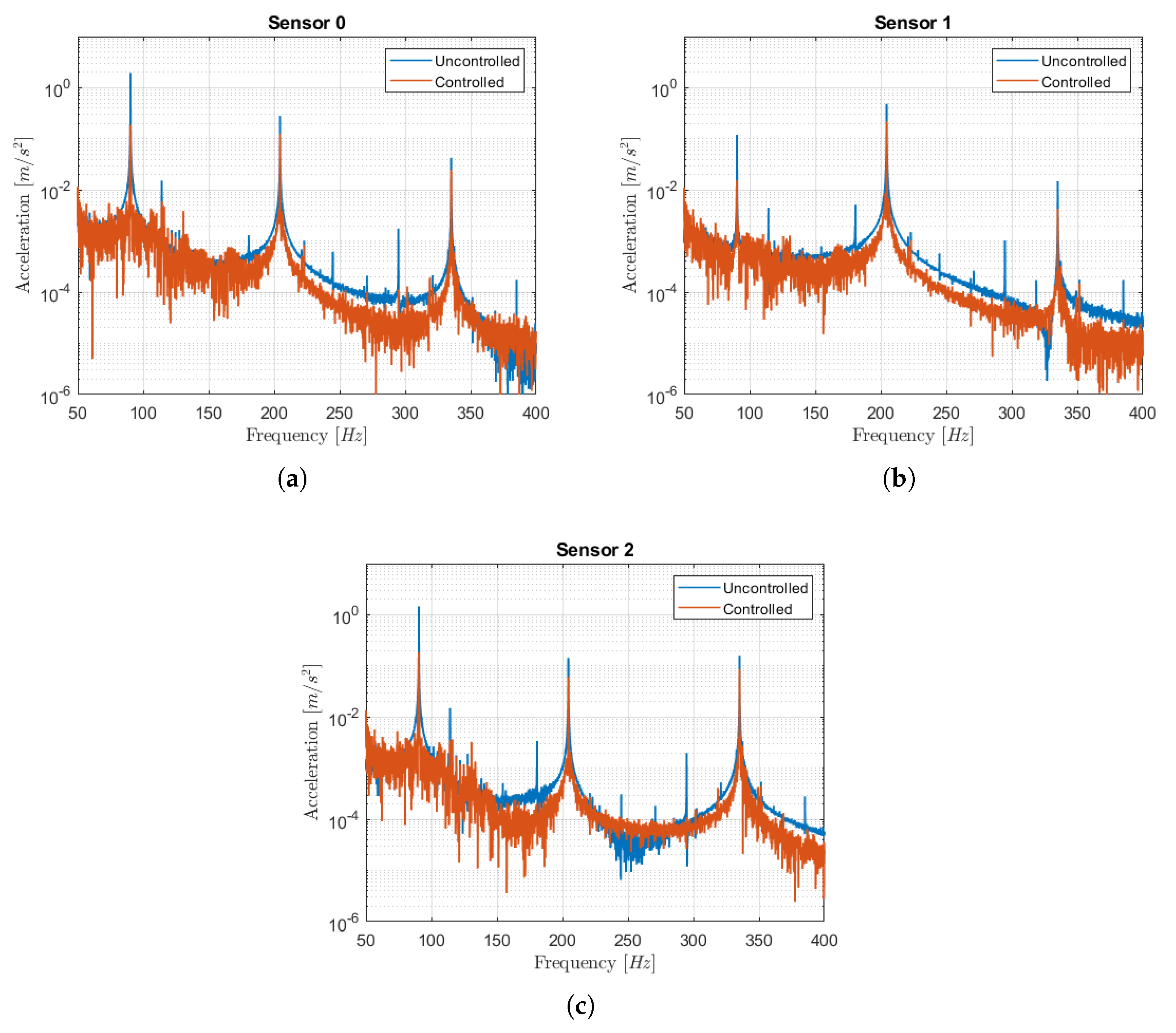
As for the numerical case, the results have been reported in

Table 7. Comparison between the vibration of the uncontrolled (blue line) and controlled (red line) system on the three sensors locations in experimental tests.

	Mode	Sensor 0	Sensor 1	Sensor 2
Uncontrolled [$\mathrm{m} {\mathrm{s}}^{-2}$]	2	1.9540	0.1205	1.463
	3	0.2826	0.4863	0.1439
	4	0.0426	0.0074	0.1585
Controlled [$\mathrm{m} {\mathrm{s}}^{-2}$]	2	0.1868	0.0154	0.1839
	3	0.1249	0.2201	0.0604
	4	0.0247	0.0043	0.0860
Reduction [%]	2	90.44	87.22	87.43
	3	55.79	54.74	58.01
	4	42.08	41.76	45.74

, showing the percentage of reduction in terms of acceleration amplitude. In Figure 7 the FRFs in the sensors positions are depicted, both for the uncontrolled and controlled case. In these plots, some fluctuations on the curves can be appreciated with respect to the numerical ones, due to the noise which affects the measurements. Then, the numerical results have been validated. The same vibration reduction has been achieved for the most excited mode (mode 2) while, for the other modes, a lower reduction has been observed. This behaviour is due to a lower value of $\gamma$ found in the experimental tests, which comes from some approximations made on the numerical model.

6. Conclusions

This work has been focused on the evaluation of modal parameters and the development of a feasible control strategy. The modified EMC strategy represents a solution that improves the vibration reduction performance with respect to a totally decentralized control system, since the global control action can be focused on some specific vibration modes according to a desired target. The goal was to reduce as much as possible the vibrations, considering also the damping that each actuator can introduce. Good results have been obtained by means of the numerical simulations, which have been validated through the experimental tests on the test rig.

The proposed solution can be customized considering also different targets with respect to the one fixed in this work. For example, a different goal could be the increase of the damping as much as possible, by using the maximum damping potential of the overall control system regardless the state of vibration. In this case, only the damping weights should be considered in the final gains setting.

The solution presented in this paper fits the project requirements, since a low computational effort and no real-time data sharing are required. This latter feature leads to an important consideration, since the main advantage of this control strategy is the scalability of the controlled system. The number of actuators can be easily increased without a reduction on the control performance, since no real-time data exchange is required to compute the control action, as centralized control architectures actually requires. To date, no fault-tolerant algorithms have been defined. Then, the control system is not robust to sensor faults, but the features of the smart devices allow the implementation of a diagnostic protocol to get information about the status of the sensors. This aspect could be addressed in future works.

Moreover, all the information needed to apply such control strategy can be obtained in the previous identification phases. Closed forms formulas, to calculate the maximum applicable gains and the weighting factors, have been derived. In particular, besides the information about structure natural frequencies and vibration state, control gains calculation requires also the knowledge of the non-dimensional damping ratio and structural gain. For this reason, a modal parameter damping estimation has been developed. In order to evaluate the damping ratio, a time-domain decay method has been applied and acceptable results have been obtained.

References

- Lewandowski, R.; Grzymisławska, J. Dynamic analysis of structures with multiple tuned mass dampers. J. Civ. Eng. Manag. 2009, 15, 77–86. [Google Scholar] [CrossRef]
- Zimmerman, D.C.; Inman, D.J. On the nature of the interaction between structures and proof-mass actuators. J. Guid. 1989, 13, 82–88. [Google Scholar] [CrossRef]
- Paulitsch, C.; Gardonio, P.; Elliott, S.J.; Sas, P.; Boonen, R. Design of a lightweight, electrodynamic, inertial actuator with integrated velocity sensor for active vibration control of a thin lightly-damped panel. In Proceedings of the 2004 International Conference on Noise and Vibration Engineering, Leuven, Belgium, 20–24 September 2004. [Google Scholar]
- Winberg, M.; Johansson, S.; Claesson, I. Inertial mass actuators, understanding and tuning. In Proceedings of the 11th International Congress on Sound and Vibration (ICSV11), St. Petersburg, Russia, 5–8 July 2004. [Google Scholar]
- Cinquemani, S.; Braghin, F. Decentralized active vibration control in cruise ships funnels. Ocean. Eng. 2017, 140, 361–368. [Google Scholar] [CrossRef]
- Zanelli, F.; Mauri, M.; Castelli-Dezza, F.; Sabbioni, E.; Tarsitano, D.; Debattisti, N. Energy Autonomous Wireless Sensor Nodes for Freight Train Braking Systems Monitoring. Sensors 2022, 22, 1876. [Google Scholar] [CrossRef] [PubMed]
- Zanelli, F.; Sabbioni, E.; Carnevale, M.; Mauri, M.; Tarsitano, D.; Castelli-Dezza, F.; Debattisti, N. Wireless sensor nodes for freight trains condition monitoring based on geo-localized vibration measurements. Proc. Inst. Mech. Eng. Part F J. Rail Rapid Transit 2022, 237, 193–204. [Google Scholar] [CrossRef]
- Zanelli, F.; Mauri, M.; Castelli-Dezza, F.; Tarsitano, D.; Manenti, A.; Diana, G. Analysis of Wind-Induced Vibrations on HVTL Conductors Using Wireless Sensors. Sensors 2022, 22, 8165. [Google Scholar] [CrossRef] [PubMed]
- Zanelli, F.; Castelli-Dezza, F.; Tarsitano, D.; Mauri, M.; Bacci, M.L.; Diana, G. Sensor Nodes for Continuous Monitoring of Structures Through Accelerometric Measurements. In Proceedings of the 2020 IEEE International Workshop on Metrology for Industry 4.0 & IoT, Roma, Italy, 3–5 June 2020. [Google Scholar] [CrossRef]
- Debattisti, N.; Bacci, M.; Cinquemani, S. Distributed wireless-based control strategy through Selective Negative Derivative Feedback algorithm. Mech. Syst. Signal Process. 2020, 142, 106742. [Google Scholar] [CrossRef]
- Debattisti, N.; Bacci, M.L.; Cinquemani, S. Implementation of a partially decentralized control architecture using wireless active sensors. Smart Mater. Struct. 2020, 29, 025019. [Google Scholar] [CrossRef]
- Debattisti, N.; Bacci, M.L.; Cinquemani, S. Application of a virtual inerter in active vibration control using inertial actuators. In Proceedings of the Sensors and Smart Structures Technologies for Civil, Mechanical, and Aerospace Systems 2020, Online, 27 April–8 May 2020; Zonta, D., Huang, H., Eds.; SPIE: Anaheim, CA, USA, 2020. [Google Scholar] [CrossRef]
- Singh, S.P.; Pruthi, H.S.; Agarwal, V.P. Efficient modal control strategies for active control of vibrations. J. Sound Vib. 2003, 262, 563–575. [Google Scholar] [CrossRef]
- Baumann, O.N.; Elliott, S.J. Decentralised control using multiple velocity feedback loops with inertial actuators. In Proceedings of the Active 2006: The 2006 International Symposium on Active Control of Sound and Vibration, Adelaide, Australia, 18–20 September 2006. [Google Scholar]
- Baumann, O.N.; Elliott, S.J. The stability of decentralized multichannel velocity feedback controllers using inertial actuators. J. Acoust. Soc. Am. 2007, 121, 188–196. [Google Scholar] [CrossRef]
- Camperi, S.; Ghandchi-Tehrani, M.; Zilletti, M.; Elliott, S.J. Multichannel decentralised feedback control using inertial actuators. In Proceedings of the ISMA 2016—International Conference on Noise and Vibration Engineering and USD2016—International Conference on Uncertainty in Structural Dynamics, Leuven, Belgium, 19–21 September 2016; pp. 1163–1177. [Google Scholar]
- Cinquemani, S.; Resta, F.; Monguzzi, M. Limits on the use of inertial actuators in active vibration control. In Proceedings of the IMETI 2011—4th International Multi-Conference on Engineering and Technological Innovation, Orlando, FL, USA, 19–22 July 2011; Volume 2, pp. 116–121. [Google Scholar]
- Zilletti, M.; Gardonio, P.; Elliott, S.J. Optimisation of a velocity feedback controller to minimise kinetic energy and maximise power dissipation. J. Sound Vib. 2014, 333, 4405–4414. [Google Scholar] [CrossRef]
- Elliott, S.J.; Serrand, M.; Gardonio, P. Feedback stability limits for active isolation systems with reactive and inertial actuators. J. Vib. Acoust. 2001, 123, 250–261. [Google Scholar] [CrossRef]
- Elliott, S.J.; Gardonio, P.; Rafaely, B.; Harris, R.; Heron, K. Performance Evaluation of a Feedback Active Isolation System with Inertial Actuators. Technical Report March; ISVR Technical Memorandum no. 832; Institute of Sound & Vibration Research: Southampton, UK, 1998. [Google Scholar] [CrossRef]
- Lindner, D.K.; Zvonar, G.A.; Borojevic, D. Performance and control of proof-mass actuators accounting for stroke saturation. J. Guid. Dyn. Control 1994, 17, 1103–1108. [Google Scholar] [CrossRef]