Abstract
Although they have achieved great success in optical images, deep convolutional neural networks underperform for ship detection in SAR images because of the lack of color and textual features. In this paper, we propose our framework which integrates prior knowledge into neural networks by means of the attention mechanism. Because the background of ships is mostly water surface or coast, we use clustering algorithms to generate the prior knowledge map from brightness and density features. The prior knowledge map is later resized and fused with convolutional feature maps by the attention mechanism. Our experiments demonstrate that our framework is able to improve various one-stage and two-stage object detection algorithms (Faster R-CNN, RetinaNet, SSD, and YOLOv4) on two benchmark datasets (SSDD, LS-SSDD, and HRSID).
1. Introduction
Ship detection has received increasing attention in the field of synthetic aperture radar (SAR) for its broad application for military [1,2,3], marine traffic monitoring [4,5], harbor surveillance [6,7], etc. Following their success in optical images, deep learning-based methods are replacing traditional methods, which rely on manually designed feature extraction, as the most popular models for SAR images [8,9,10,11,12,13]. Among the deep learning methods, deep convolutional neural networks (CNNs) overwhelm other branches in the computer vision.
Despite the popularity of CNNs for various tasks of SAR images, ship detection remains a challenging task for three reasons. Firstly, SAR images do not have important features, such as color and textual features, which are vital for object detection. Secondly, ships are normally quite small in SAR images. Therefore, resolutions are too small to easily locate ships [14,15,16,17]. Thirdly, for complex backgrounds (e.g., coast), ship detection is heavily affected by the scattering points from the background [6,18,19,20,21].
Although the imaging mechanism of SAR images poses great obstacles, it provides supplementary information for ship detection. In most cases of SAR images, the backgrounds of ships are water surface (e.g., ocean, river) or coast. On the one hand, due to complex scatterings from the ships, such as volume scattering and double-bounce, the intensity of echoes generated by ships is significantly stronger than that of the water surface [22,23]. On the other hand, due to the structure and material of the ship, the ship has many strong scattering objects [24], i.e., strong scattering points. Studies [25,26] have shown that the strong scattering points of the ship are more dense than the surrounding areas.
Over the recent years, a series of explorations have been proposed to combine prior knowledge with deep learning methods. Gao et al. [27] extracted the SAR polarization features [28] using the power–entropy (PE) decomposition theory. After that, the polarization features were fed into RetinaNet [29] as the input. Zhang et al. [30] defined the saliency value of a pixel as the color contrast of all other pixels in the image. They generated high-quality slices using a saliency detection method to suppress background clutter, before using CNNs to further detect ship targets. Their method substantially improved the detection capability of offshore ships while ensuring the inshore ship detection performance. However, due to the over-suppression of saliency detection, their method did not perform well when facing small ships with very few pixels. Sun et al. [31] pointed out that the general deep learning-based detectors perform poorly because they ignore the characteristics of SAR images. They grouped all the extracted strong scattering points, and generated the initial ROI areas based on the grouping result. Compared to those extracting only a portion of strong scattering points as key points, Sun et al.’s method performed better for small targets. However, the method of getting the initial ROI at the beginning of training was trained insufficiently, which makes the initial ROIs inaccurate and causes the model to fail to learn valid knowledge. Although previous works recognize the importance of prior knowledge for the CNNS, they combine the prior knowledge by feeding it into the networks. Therefore, the networks could not access the raw information which may be missing from the prior knowledge.
In this paper, we propose a framework which integrates prior knowledge into CNNs by fusing it with an attention mechanism. In our model, the prior knowledge is used to guide the attention of deep networks. Our framework can be categorized into two stages: prior knowledge representation and prior knowledge integration. The aim of the first stage is to generate the probability score for each pixel of which how likely it is on the ship area or background. Based on the findings from other works [28,31,32], brightness and density are two promising features for prior knowledge. To this end, we employ k-means clustering as brightness filtering because there are ships and backgrounds in a bounding box. Similarly, DBSCAN clustering is utilized as the density filtering. For the second stage, we down-pool the original prior knowledge map into the same size as the feature map. After that, position-wise multiplication integrates the resized prior knowledge map into the CNNs.
Our contributions can be summarized into three items.
- To our best knowledge, our framework is the first that can integrate prior knowledge into arbitrary CNN-based detectors using attention mechanism for SAR images.
- By the attention mechanism, the deep learning models can learn from both prior knowledge and vanilla images.
- Our experiments exhibit the superiority of our method using object detection algorithms (Faster R-CNN, RetinaNet, YOLOv4, and SSD) on three SAR image datasets (SSDD, LS-SSDD, and HRSID).
The remainder of this paper is organized as follows. Section 2 presents the related works about traditional methods, CNN-based object detection algorithms, and attention mechanisms. Section 3 details our intuition and approaches to represent prior knowledge. Section 4 demonstrates the combination of prior knowledge and deep CNNs. Section 5 displays the settings, descriptions, and results of our experiments.
2. Related Work
2.1. General CNN-Based Object Detection
Neural networks have a family of variants, including convolutional neural networks (CNNs) [33], recurrent neural networks (RNNs) [34], auto-encoders [35,36], transformers [37,38], etc. CNNs are one of the most vital branches that are widely applied in computer vision tasks, including object recognition [39], object detection [29,40,41,42], segmentation [43], and image generation [44]. CNN-based object detectors can be grouped into single-stage and two-stage algorithms. Faster R-CNN [45] is one of the most widely used two-stage detectors, which is an extension of Fast R-CNN [42]. The Faster R-CNN replaces the selective search of Fast R-CNN with region proposal networks (RPN). The RPN enables the end-to-end training and further reduces the computational complexity. The single-stage algorithms do not rely on proposed regions, such as typical single-stage algorithms YOLO [41,46,47], SSD [48], and RetinaNet [29], which perform classification and regression directly from feature maps. The YOLO [46] models the detection task as a pure regression problem. It divides the image into grids of patches, and performs the prediction and classification of the bounding boxes for the center of each grid. The core of RetinaNet [29] is focal loss, a loss function derived from a modification of binary cross-entropy. Focal loss makes the model more focused on hard-to-classify samples during training by reducing the weights of easy-to-classify samples. YOLOv4 [41] uses PANet [49] instead of the commonly used FPN as the neck of the network and assembles various optimization strategies for CNNs, including Mosaic data augmentation method, Mish activation function [50], and CIoU loss function [51], to improve the detection accuracy of the algorithm.
In the deep learning era, the CNNs have dominated the object detection in SAR images. Lv et al. [52] combined a sliding window and Faster R-CNN approach to detect pylons in SAR images and used a data enhancement strategy to train it. Their detector has good immediacy and detection rate in large-scene SAR images. Ge et al. [53] improved the feature extraction capability of the algorithm for azimuthally inscribed objects by adding SENet and inverted residuals to the backbone of YOLOv5. Their proposed detector was suitable for detecting azimuthally sensitive targets, such as aircraft. Zhang et al. [54] cross-coupled the edge-aware network by a residual space pyramid set and attention mechanism to help object recognition. In addition, they improved the model’s multi-scale feature extraction capability by semi-dense connectivity based on residual convolution blocks. Their proposed SAR image detector performed well on SAR oil tank and residential area images. Sun et al. [55] used transformer to build the neck of YOLOv5. They found out that adding the structure of transformer in the high level of YOLOv5 can help the model to obtain global background information, which improved the performance of YOLOv5. This method achieved good results in detecting military vehicles in large scenarios.
Deep CNNs have made a lot of breakthroughs for ship detection in SAR images as well. Tang et al. [8] proposed a new ship detection model FLNet based on YOLOv5. This model combined traditional image processing and deep learning-based methods, with improved accuracy and recall. Zhu et al. [9] used FCOS as the baseline, redesigned the feature extraction method, and redefined the sample according to the statistical features of SAR ships to reduce the missed detection rate of small ships. Li et al. [10] replaced the original RPNs with a fixed number of prior anchor boxes with K-means, applied cascade amplification and feature fusion to design the feature extraction network, and improved the speed and accuracy of the Faster R-CNN. To effectively aggregate the sparse and meaningful clues of small ships, Shi et al. [11] introduced a deformable attention mechanism based on the Swin Transformer to change the original self-attention mechanism. Yu et al. [12] constructed a highly accurate and highly generalizable network, FIERNet, by combining feature extraction and fusion modules. The differentiable neural structure search model proposed by Li et al. [13] employs a new channel cropping scheme and loss function that can generate significantly lighter neural networks with guaranteed accuracy.
2.2. Prior Knowledge for Detection SAR Images
Before the popularity of deep learning, constant false alarm rate (CFAR) was one of the most seminal feature extraction methods [56] for object detection in SAR images. CFAR is a statistical detection method based on hypothesis testing theory, which ensures a constant false alarm probability by selecting a suitable threshold, and then determines whether the target signal exists under this condition. The MS-CFAR [57], which takes into account the statistical characteristics of the tested cell, has a more stable performance compared to other algorithms based on CFAR. The statistical clutter edge selector designed in [58] can obtain a uniform clutter field before CFAR, improving the detection performance of the classical CFAR detector. Moreover, the idea of improving the algorithm by using clutter boundary statistical features is also reflected in [59]. The bi-parametric clutter map CFAR detection method proposed by Wang et al. [60] estimates the local threshold by following the standard deviation and mean values of the new clutter map, which has better applicability and target detection capability compared to the mono-parametric method. Zhou et al. [61] chose to use the half-sided Gaussian distribution for modeling and proposed a new method called HG-CFAR. This method has higher efficiency relative to the CFAR method based on a Gaussian distribution.
Specifically, there is a group of works which are for ship detection only. Li et al. [62] found that the grayscale values on SAR images fluctuate due to the influence of speckle noise. Such fluctuations take a regular form in uniform regions and an irregular form in non-homogeneous regions. The ship region is a homogeneous region while the ship boundary region and the artificial target are non-homogeneous regions. Based on this phenomenon, they designed a new texture feature IUDF for helping ship detection in SAR images. The proposed algorithm using IUDF has high accuracy and processing speed. The ship, as a scatterer, has a strong coherent backscattering signal, and this feature can be formed by evaluating the sub-resolution electromagnetic field, in which Gambardella et al. [63] considered the Rice factor as a parameter that is sensitive to a dominant scatterer such as a ship. Therefore, they designed a filtering technique based on the Rice factor, by which the accuracy and efficiency of the ship detection algorithm can be effectively improved. Zhang et al. [64] also designed a filtering technique for SAR ships, but their technique was based on the strong double-bounced scattering phenomenon occurring from ships. In [65], the authors found that the azimuth ambiguities caused by the undersampling of the echo signal during SAR imaging can lead to false alarms of ships. As a result, they located and eliminated the ambiguous points in SAR images in advance according to the imaging coefficients of SAR, as a way to reduce the interference of orientation-ambiguous points to SAR ship detection.
2.3. Attention Mechanisms
Attention mechanisms make the model focus on more critical features. Squeeze-and-Excitation Networks (SENet) [66] and Convolutional Block Attention Module (CBAM) [67] are two of the most popular attention mechanisms. SENet computes channel weights by compressing the information of all points in the space and uses the fully connected layer to exploit the correlation between channels, effectively improving the accuracy of the network. In [68,69], the researchers added SENet to the feature extraction network to enhance the representation of vehicle features. Compared to SENet, which simply uses the channel attention mechanism, CBAM additionally uses the spatial attention mechanism. One of the advantages of CBAM is that it is plug-and-play and can be easily incorporated into various algorithms. Zhu et al. [70] integrated CBAM into YOLO to help YOLO better find regions of interest. Wang et al. [71] made their VGG-style network more focused on effective features by embedding CBAM. Feng et al. [72] combined CBAM with SSD to effectively suppress useless information and improved the pedestrian detection accuracy of the algorithm.
Attention mechanism has been extensively used for object detection in SAR images. Zhang et al. [73] designed a lightweight attention mechanism which has significant performance and efficiency for the detection task of multi-class SAR targets in both moving and stationary situations. Combined with feature pyramids, SENet achieved competitive performance in the SAR bridge detection [74], because the SENet enables detectors to suppress irrelevant information while obtaining additional valid information. Guo et al. [75] used a mixture of feature pyramid networks and CBAM to further process the features enhanced by scattering information, effectively adapting to the discrete and variable nature of aircraft in SAR images.
Attention mechanism is useful for ship detection as well. The ship attention module proposed by Sun et al. [21] distinguishes the strong scattering points of artificial facilities on land and ships in water by generating a feature map containing rich texture features, which effectively reduces false alarms in the land area and improves the accuracy of the algorithm. Wang et al. [7] designed a Spatial Group-wise Enhance (SGE) attention module to reduce the problem of adjacent ships being ignored. SGE reduces the computational effort in the form of channel grouping, while enhancing the spatial features of each group of channels, providing more semantic features. Their experimental results showed that their method has better detection capability for densely docked ships and makes a contribution to ship detection in complex scenarios. Shao et al. [76] designed a dynamic shrinkage attention mechanism to address the impact of speckle noise on SAR images, which can automatically learn the soft threshold required by the denoising algorithm to achieve feature-level denoising.
3. Representing Prior Knowledge
3.1. Analysis
SAR images are different from optical images due to different imaging mechanisms. Optical images record multi-band data, while SAR images record single-band data, such as the amplitude and phase of one band of echoes. Therefore, SAR images are usually single-channel pictures, which have a pixel value range of 0 to 255, inclusively. The digital image element, or pixel value, reflects the intensity of the scattered echoes before the imaging. The stronger the echo signal, the larger the pixel value is. Figure 1 visualizes ships in optical images (first row) and SAR images (second row), respectively. In the optical images, we can easily locate ships by the contour, color differences, and texture. However, there is a large amount of speckle noise in SAR images, and the ship targets are usually blurred. Ship targets in SAR images not only lack rich color information, but also possess unclear texture features. This delivers difficulties for the detection of ships in SAR images.
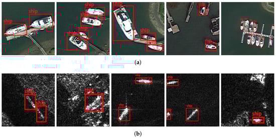
Figure 1.
Examples of optical and SAR images, with the ship target marked by the red rectangle. (a) Optical images. (b) SAR images.
The intensity of scattered echoes roughly depends on two types of factors [77]. The first factor is the operating parameters of the radar system, including the operating wavelength of the radar sensor, the angle of incidence, the polarization mode, etc. The second factor is the characteristics of the ground target, including the roughness of the ground surface, the radar scattering cross section (RCS), the complex permittivity of the target, etc. They mainly affect the type of scattering occurring from the target and thus the intensity of the scattered echoes [77,78,79,80]. Ships generally have simultaneous volume scattering, surface scattering, and double bounce [81]. The echoes generated by double-bounce are very strong. Even if only surface scattering is considered, the echoes generated by the ships will be stronger than those from the sea surface. We refer to this phenomenon as the brightness difference. Figure 2 illustrates this phenomenon. The ships look significantly brighter than the sea surface.
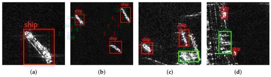
Figure 2.
Ships with different background in SAR images. Ships are significantly brighter on SAR images than on the sea surface. The ship targets are marked in red boxes, and the strong scattering points on land are marked in green boxes. (a) Example 1 of ship’s brightness. (b) Example 2 of ships’ brightness. (c) Example 3 of the brightness difference between ships and land. (d) Example 4 of the brightness difference between ships and land.
From Figure 3, we can conclude the strong scattering points on land also produce high-intensity echoes, which leads to the pixels on the SAR image having similar brightness as ships. Therefore, brightness alone is not enough to distinguish ships from the background. SAR imaging has the inherent defect of coherent speckle noise [82]. In SAR images, the grayscale values of neighboring pixel points can vary randomly due to coherence, which is around a certain mean value. As a result, a uniform scatterer can also appear to vary unevenly between bright and dark on a SAR image. Targets with different structures are affected differently by speckle noise due to the different distributions of the basic scatterers in their bodies. We describe this phenomenon in terms of the density of bright spots in the region. From Figure 3, we can discover that the density of the bright spots of the ships in the red boxes is significantly higher than that of the background in the green boxes.
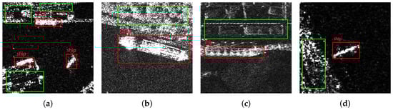
Figure 3.
Objects with different densities in the SAR images. The difference in densities comes from the difference in structures. The red boxes in the figure mark the ships while the green boxes mark the areas. The densities of land are significantly different from those of the ships. (a) Example 1 of density difference between ships and land. (b) Example 2 of density difference between ships and land. (c) Example 3 of density difference between ships and land. (d) Example 4 of density difference between ships and land.
3.2. Generating by Brightness
As aforementioned in Section 3.1, brightness is important to distinguish ships from the water surface. Therefore, we can use an interval of pixel values to separate ships from the water surface. Only pixels within are considered as ships. Since the images from training set and test set are i.i.d., the interval which fits for the training set suits the test set as well.
We perform clustering on pixels of each bounding box (annotations of training set) individually. we use K-means [83] clustering with two classes (one for the foreground and the other for the background) to cluster the pixel values. The cluster which has a higher value as the center than that of the other cluster represents the foreground. From the foreground pixels, we find a pair of median value and max value , where i indicates the global index of bounding boxes. The global median value and max value could be calculated as:
Here, n is the total number of bounding boxes. The final interval is .
As can be seen from Figure 4, most of the points in the clustering results are distributed at higher pixel value levels. It can be illustrated that most pixels in the bounding boxes represent ships while others are noises. The intervals from Equations (1) and (2) visualized on the second row suggest the effectiveness of our approach.
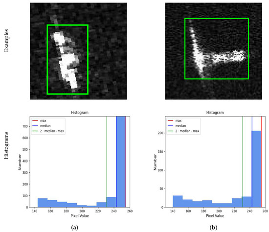
Figure 4.
Two ship examples and their histograms. In the example, only the pixels in the green box (on the images from first row) are included in the distribution for the second row. (a) Ship pixel distribution example 1. (b) Ship pixel distribution example 2.
3.3. Generating by Density
As discussed in Section 3.1, brightness is insufficient to separate ships from land, but density is a promising feature, because the pixels on the ships are more dense than that on land. We use DBSCAN [84] for the filtering in this stage. The input of the DBSCAN is the foreground pixels of the brightness filtering. DBSCAN owns two hyper-parameters to tune: and . Two points are considered neighbors only if the distance between them is no bigger than . A core point has at least points in its neighbors.
Instead of adopting the strategy introduced in the original paper [84], we use the metric IoU to tune the hyper-parameters. Experiments are conducted using different combinations of and , and the final set of parameters with the highest IoU is selected. The IoU of a single image and the IoU of the whole dataset are calculated as shown in Equations (3) and (4):
In Equation (3), U represents the number of points where the clustering result overlaps with the real ship. X represents the number of points in the clustering result. represents the number of real ship points. In Equation (4), n is the total number of images. represents the IoU of the ith image. represents represents the number of targets on the ith image.
After sequentially applying K-Means clustering and DBSCAN clustering, for each pixel on the SAR images, we obtain a binary value for it. A pixel with value one is considered a part of ship, while a pixel with value zero is taken as background. Such matrix is denoted as prior knowledge map because the values are calculated based on prior knowledge of SAR images. The prior knowledge map has the same size as the SAR image but with a single channel.
4. Combining Prior Knowledge Map
Figure 5 depicts the comprehensive architecture of our framework. The framework has three important parts: the backbone, our attention component (BDAM), and the prior knowledge map. The backbone can be ResNet [85], VGG [86], GoogleNet [87], etc. Our attention component (BDAM) does not change the sizes of the input and output of the backbone. We insert it between stages of the backbone. The shape of the input and output of BDAM is equally the same.
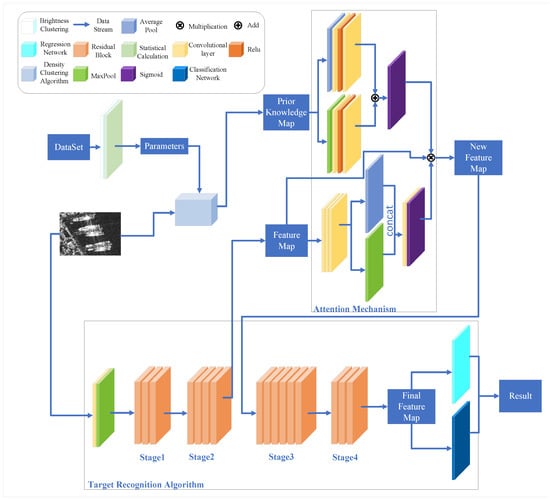
Figure 5.
The comprehensive architecture of our framework. It consists of backbone, BDAM, and a prior knowledge map.
4.1. Resizing Prior Knowledge Map
The diagram of our attention component is depicted in Figure 6. The original prior knowledge map, on which each point indicates if it is foreground or background, has the size of . In order to be attended with the feature map, we need to convert the prior knowledge map to the same size as the feature map. Let us assume that a feature map has the size . We divide the original prior knowledge map into windows, where and .
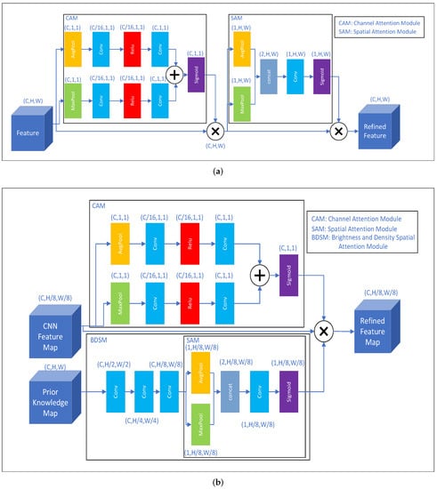
Figure 6.
Comparison of CBAM and BDAM. (a) CBAM. (b) BDAM.
The value of each window is the number of foreground points within. Intuitively, the window with more foreground points requires more attention. We normalize the counting of foreground points into as the confidence score. The process of converting the original prior knowledge map into the resized prior knowledge map is depicted in Figure 7.
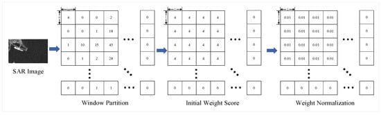
Figure 7.
The schema of resizing the prior knowledge map. Details include regional division, core point statistics, assigning the initial weight, and weight normalization.
4.2. Integrating Prior Knowledge Map
Traditional attention mechanisms (such as SENet) serve as self-attention, which have one input tensor. In our work, there are two input tensors: one is for the resized prior knowledge map; and the other is the feature map of CNNs. The output tensor is considered as a better representation of the feature map of CNNs. The output is fed into latter stages of the CNNs.
Our BDAM extends the structure of CBAM. The detailed structure of BDAM is shown in Figure 6. Given an intermediate feature map, CBAM (depicted in Figure 6a) successively infers attention maps along two separate dimensions, channel and spatial. After that, the attention maps are multiplied to the input feature map for adaptive feature refinement. Our module (BDAM) uses the CNN feature map for channel attention and the prior knowledge map for spatial attention (Brightness and Density Spatial Attention Mechanism, BDSM), which is shown in Figure 6b.
The intermediate CNN feature map and the prior knowledge map are used as the input of BDAM. is passed through the channel attention mechanism to obtain the channel attention weight , while is passed through the spatial attention mechanism to obtain the spatial attention weight . The channel attention weight and spatial attention weight are multiplied to get the final attention weight . This process can be described as:
where ⊗ represents the element-wise multiplication, and is the feature map after adjusting the weights.
The channel attention module can be divided into two branches: max-pooling and average-pooling. Max-pooling and average-pooling operations are performed on the CNN feature maps to obtain and . and are fed into the multilayer perceptron (MLP), and the two results output by the MLP are summed element-wise. The merged tensor is finally passed through the Sigmoid function to obtain the channel weights. This process can be described as:
where , represent the weights of the MLP, and r is the reduction ratio.
In the BDSM, the prior knowledge map is first resized by a multilayer convolutional neural network. The resized prior knowledge map is subjected to maxi-pooling and average-pooling operations in the channel direction. Then, the outputs and of the two branches are concatenated and fed into a convolutional layer with a convolutional kernel of size . The spatial attention weights are calculated as:
where represents the weights of the initial layers of convolution and f represents the last layer of convolution.
5. Experiments and Results
5.1. Environment
Our experiments are conducted with one Tesla V100 DGXS 32GB GPU. The operating system was Ubuntu 18.04. We used PyTorch 1.8.0, cuda 11.6, and cudnn 7.6.5 as our GPU platform.
5.2. Datasets
The datasets used in the experiment are SSDD [88], LS-SSDD [89], and HRSID [90]. These datasets contain SAR ships only. SSDD has 1160 images with 2456 ships. SSDD derives from three satellites: RadarSat-2, TerraSAR-X, and Sentinel-1, which display ships at multiple scales and in multiple scenarios. The HRSID comes from three radar satellites: TerraSAR-X, TanDEMX, and Sentinel-1B, with a total of 5604 images containing 16,951 ships. The data of LS-SSDD are from one satellite, Sentinel-1, with a total of 9000 images. The three datasets are annotated as the format of PASCAL VOC. The size of ships within these three datasets varies widely. According to the MS COCO [91] definition of target size, LS-SSDD consists of no big ships and almost small ships, while SSDD and HRSID contain various sizes of ships. Table 1 demonstrates the details of the three datasets. Because of the scarcity, SAR datasets are smaller than other detection datasets, such as COCO which contains 328,000 images.

Table 1.
Statistics of datasets.
For the SSDD, we follow the data split instructed by its owner [92]. Those images with a tail number between 2 and 7 or 0 are divided into the training set, while those with a tail number of 8 are used for validation during the training process and, finally, the remaining images are used for testing. The division of validation, test, and training sets in the HRSID dataset is randomly divided according to 1:1:8. The authors of LS-SSDD gave a fixed division of the dataset into a training set of 6000 and a test set of 3000. In the experiments of this paper, we randomly delineated 1000 from the 6000 training sets as the validation set. Table 2 shows the number of images for different purposes after the division of the three datasets.
Table 2.
Distribution of datasets.
5.3. Implementation Details
In this experiment, the backbone networks of all algorithms are loaded with parameters pretrained on the ImageNet dataset. Among them, the backbone networks of the algorithms are ResNet50 except for YOLOv4 whose backbone network is CSPDarkNet53 [41]. Faster R-CNN and RetinaNet additionally add FPN as the neck of the network.
The optimizer used in the training process is SGD, whose parameters and are set to 0.937 and 0.0001. The training epochs of the other three algorithms are 25, except for YOLOv4 where the training epochs are 200. The data augmentation strategies used in training the four algorithms are RandomFlip and Resize. MixUp and Mosaic data augmentation strategies are additionally used in the YOLOv4 training, where Mosaic is only used in the first 70% of epochs (140 epochs).
5.4. Evaluation Criteria
Following the convention of MS COCO [91], we adopt the following six metrics for evaluation: (Average Precision), , , , , and . , are the AP values obtained with IoU fixed at 0.5 and 0.75. , , and calculate the average AP values for all small, medium, and large targets, respectively.
5.5. Hyper-Parameter Analysis
As mentioned in Section 3.3, clustering parameters are the key point of the attention mechanism. Table 3 displays the brightness intervals of the ships obtained with brightness clustering in the datasets.
Table 3.
The brightness intervals of SSDD, LS-SSDD, and HRSID.
From the table, we observe that the same class of targets may have different brightness intervals in different datasets. The cause is the different system parameters used in the acquisition of different datasets. Therefore, it is necessary to use brightness clustering to learn the brightness intervals of the targets in the dataset in advance.
Figure 8 shows the performance of different and on three datasets. The more leftward the horizontal coordinate in this graph, the smaller the ratio of to . It can be found that as the ratio rises, the curves of SSDD and HRSID will first rise to a certain value and then start to fluctuate in a small range, while the curve of LS-SSDD starts to fall after fluctuating for a period of time. According to the trend of the curve changes in Figure 8, the combination used for the experiments on SSDD is and , while the combination of and is used for the experiments on HRSID. And for the LS-SSDD, we choose the combination of and . Using these parameters, the average IoUs obtained on SSDD, LS-SSDD, and HRSID are 0.754, 0.463, and 0.632.
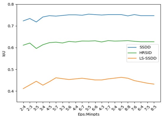
Figure 8.
The performance of different and on SSDD and HRSID. The vertical coordinate is the value of IoU and the horizontal coordinate is : .
Figure 9 is the visualization of the clustering results on some images in the training datasets. For the image of ships on the sea, the filtered points are all on the ships. Even for a complex background as in the image of ships near the shore, our approach filtered out most noisy points.
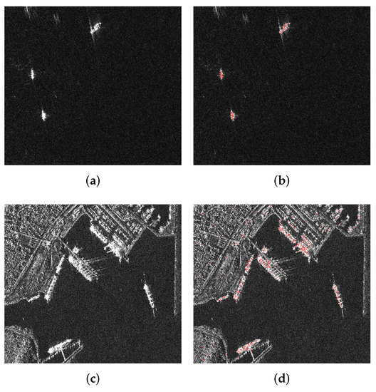
Figure 9.
Display of partial clustering results on pictures. Ships from clustering are in red. (a) Original image of ships on the sea. (b) Clustering results for the ships on the sea. (c) Original image of ships near the shore. (d) Clustering results for the ships near the shore.
5.6. Time Analysis
We test the time required to represent and combine the prior knowledge individually. Table 4 and Table 5 detail the total time spent, the average time spent per image, and the FPS for the different programs in the two phases. The images used to test the time performance are from the training set of SSDD, with a total of 812 images.
Table 4.
Time consumption for representing the prior knowledge.
Table 5.
Time consumption of combining the prior knowledge with SSD.
Representing the prior knowledge includes calculating metrics (e.g., IoU metrics of DBSCAN) for better hyper-parameter selection, which is approximately eight times slower than combining the prior knowledge. However, because the hyper-parameters are preserved during training and inference of models, the heavy cost is one-off and is the disposal in time complexity. Table 5 demonstrates the complete elapsed time for generating and representing prior knowledge as well as the elapsed time for each component during training and inference. The complete program takes an average of 0.0223 seconds to process an image on the GPU and achieves an FPS of over 44.
5.7. Qualitative Results
To prove the validity of BDAM, we add it to four popular detectors (Faster R-CNN, YOLOv4, RetinaNet, and SSD) for experiments and compare it with the original algorithms. In addition, we compare the effects with attention mechanisms EAM [17], BCA [93], and CBAM [67]. The first two are specially designed for SAR images while the last one is one of the most popular for general purpose.
Table 6, Table 7 and Table 8 show the performance of these four algorithms on the three datasets, where the bold data represent the one with the best results for a certain metric of the same algorithm, and the underlined data represent the one with the second best results. Figure 10 and Figure 11 show the recognition results of some images.
Table 6.
Experimental results of different algorithms on dataset SSDD. Bolded data represent the best and underlined data represent the second best.
Table 7.
Experimental results of different algorithms on dataset HRSID. Bolded data represent the best and underlined data represent the second best.
Table 8.
Experimental results of different algorithms on dataset LS-SSDD. LS-SSDD does not contain large ships, so the metrics of do not apply to it. Bolded data represent the best and underlined data represent the second best.
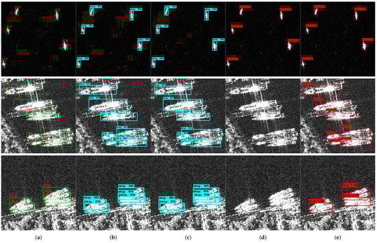
Figure 10.
Ground truth and recognition results of some images. (a) Ground truth. (b) Faster R-CNN. (c) Faster R-CNN with BDAM. (d) YOLOv4. (e) YOLOv4 with BDAM.
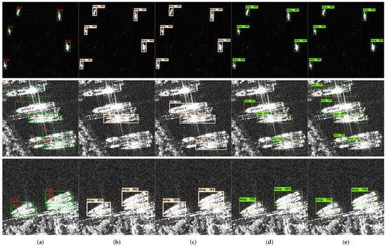
Figure 11.
Ground truth and recognition results of some images. (a) Ground truth. (b) SSD. (c) SSD with BDAM. (d) RetinaNet. (e) RetinaNet with BDAM.
As illustrated in Table 6, Table 7 and Table 8, BDAM performs well with all detectors on all three datasets. Namely, the BDAM achieves 10 winners and 2 runners-up with Faster R-CNN; 9 winners and 2 runners-up with RetinaNet; 10 winners and 2 runners-up with SSD; and 7 winners and 2 runners-up with RetinaNet. We can notice that all baselines have a stable improvement on the detection ability of large targets after adding BDAM. For example, on the SSDD data, RetinaNet’s improves by 7.7% after adding BDAM while it improves by 9.2% on the HRSID dataset, which is a significant improvement.
Table 6 and Table 7 reveal that performance of each method on is better than that of and . Although there is no large ship in Table 8, the performance of is better than . In addition, from the three tables, we observe that the improvement of our model is insignificant on . It indicates that the detectors we used learned features well on medium size targets. BDAM could not improve detectors further if sufficient information has been utilized.
On SSDD (Table 6), BDAM combined with YOLOv4 underperforms other combinations. Unlike other detectors, YOLOv4 uses Mosaic as one of its data augmentation strategies. Mosaic extends CutMix by mixing four images at a time as one training image, which aims to enrich the background. However, the reality images are likely to contain no objects, which is equivalent to adding a lot of noise to the training process of the model. Adding appropriate noise to the training process can be beneficial to prevent the model from overfitting. However, it hinders BDAM. If an image does not contain objects, then the prior knowledge map obtained by clustering is likely to be an all-0 image. It makes BDAM not work well but increases the training burden of the model. Therefore, we follow the YOLOX [47] approach. Instead of using Mosaic in all epochs, we only use Mosaic in the first 70% epochs. However, limited by the amount of data, BDAM still does not perform as well on SSDD as it does on HRSID.
5.8. Ablation Study
5.8.1. Insertion Strategy
The insertion of BDAM can be divided into two ways, one is inserted between the backbone’s stages, and the other is inserted into the backbone’s blocks. BDAM does not fit into the second scheme. There is a big difference between BDAM and CBAM: the input of spatial attention in BDAM is the prior knowledge map while the input of CBAM is the output of the upper convolutional layer. If we want to insert BDAM into the block, it is not as easy as CBAM, and we have to solve the input problem for each block. For one input image, only one prior knowledge map can be generated. It means that we need to generate multiple weight maps of different sizes from a single prior knowledge map, which sounds like feeding a single image into a convolutional neural network to obtain a multi-scale feature map. However, the prior knowledge map is different from images, which are obtained by clustering based on our prior knowledge, and it contains certain interpretability itself. However, if it is fed into a very deep network to extract weighted graphs at multiple scales, we cannot guarantee whether the knowledge recorded on the prior knowledge map can be retained. Moreover, the insertion of BDAM into the block causes the effect of pre-trained parameters to be affected. According to He et al.’s study [94] on pre-trained parameters, the amount of data in HRSID and SSDD does not support us to train from scratch. The data in Table 9 confirm our concerns, where the BDAM with * represents the insertion into the block.
Table 9.
Performance of insertion in block and insertion in stage on Faster R-CNN. Bolded data represent the best and underlined data represent the second best.
If we take the first way, since the size of the feature map output from each stage is different, we can change the problem to which size of the feature map we should adjust with BDAM. We conduct experiments on SSDD using Faster R-CNN. The backbone used in the experiments is ResNet50, and the results of the experiments are shown in Table 10.
Table 10.
Experimental results of different size weighting maps. Bolded data represent the best and underlined data represent the second best.
According to the experimental results, we find that using BDAM to adjust the feature maps that are reduced by a factor of 8, each relative to the initial input length and width, works best. That is, it is better to insert BDAM between the second stage and the third stage.
5.8.2. Attention Components
BDAM is a hybrid attention mechanism, in which the channel attention mechanism follows the implementation of CBAM. Our innovation and work focus on the spatial attention mechanism of BDAM. We call our spatial attention mechanism Brightness and Density Spatial Attention Mechanism (BDSM). Previous comparative experiments can only prove the effectiveness of BDAM, but are not enough to prove the effectiveness of BDSM.
To demonstrate the effectiveness of BDSM, we design the ablation experiments. The accuracy of the four algorithms with only the channel attention mechanism, only BDAM, and only BDSM is compared. In addition, spatial attention in CBAM uses the feature map output at the upper layer of the feature extraction network as input, which is very different from BDSM. Therefore, we also compared it with CBAM in the ablation experiment to demonstrate the effect of the prior knowledge map. Table 11 presents the results of the ablation experiments. The only dataset we used in the ablation experiment is HRSID.
Table 11.
Comparison of BDSM with different attention mechanisms. Bolded data represent the best and underlined data represent the second best.
Comparing BDSM with BDAM, under four baselines and six evaluation criteria, BDAM wins a total of 12 winners and 9 runners-up, while BDSM wins a total of 11 winners and 8 runners-up. BDSM performs similarly to BDAM, and even slightly better than BDAM occasionally. For example, BDSM achieves 4 winners and 2 runner-ups in RetinaNet, and 3 winners and 1 runner-up in metrics. BDAM adds CAM to BDSM, but BDAM has a humble improvement over BDSM. It indicates that BDSM plays a much larger role than CAM in BDAM.
Comparing CAM with BDAM, the effect of adding CAM is worse than adding BDAM for all metrics of different baselines. BDAM adds BDSM to CAM, and its effect has been greatly improved. This suggests the effectiveness of BDSM. The difference between BDAM and CBAM is the different spatial attention mechanisms, and BDAM beats CBAM in all metrics and baselines. This also shows that BDAM’s spatial attention (BDSM) is superior to CBAM’s spatial attention.
From the above comparative experiments, we believe that BDSM is effective and plays a major role in BDAM.
6. Discussion
Overall, our paper establishes a simple way of integrating prior knowledge into the CNN-based detectors by attention mechanisms. Through analyzing the ships in SAR images, we discovered that clustering extracts the prior knowledge easily. From the extensive experiments, we demonstrate that BDAM could be successfully applied to various CNN-based detectors easily. For example, on the SSDD data, RetinaNet’s improves by 7.7% after adding BDAM while it improves by 9.2% on the HRSID dataset, which is a significant improvement. Furthermore, the ablation study implies that the most important component in the BDAM is BDSM.
However, the limitation of the BDAM is obvious. As a proof-of-concept, our prior knowledge is constructed by the fact that backgrounds in most images are shores or water surfaces for ship detection. The task is hard to escalate into general object detection in SAR images.
Author Contributions
Conceptualization, Y.P. and L.Y.; Methodology, Y.P. and L.Y.; Software, Y.P.; Validation, Y.P.; Formal analysis, Y.P.; Investigation, Y.P.; Resources, Y.P. and J.L.; Data curation, Y.P.; Writing—original draft, Y.P.; Writing—review & editing, L.Y. and Y.X.; Visualization, Y.P. and L.Y.; Supervision, L.Y. and Y.X.; Project administration, L.Y.; Funding acquisition, Y.X. All authors have read and agreed to the published version of the manuscript.
Funding
This research was funded by the Zhejiang Provincial Natural Science Foundation of China, grant number LY20F020029.
Institutional Review Board Statement
Not applicable.
Informed Consent Statement
Not applicable.
Data Availability Statement
Not applicable.
Conflicts of Interest
The authors declare no conflict of interest.
References
- Brusch, S.; Lehner, S.; Fritz, T.; Soccorsi, M.; Soloviev, A.; van Schie, B. Ship surveillance with TerraSAR-X. IEEE Trans. Geosci. Remote Sens. 2010, 49, 1092–1103. [Google Scholar] [CrossRef]
- Zhao, Z.; Ji, K.; Xing, X.; Zou, H.; Zhou, S. Ship Surveillance by Integration of Space-borne SAR and AIS—Review of Current Research. J. Navig. 2014, 67, 177–189. [Google Scholar] [CrossRef]
- Paes, R.L.; Lorenzzetti, J.A.; Gherardi, D.F.M. Ship detection in the Brazilian coast using TerraSAR-X SAR images. In Proceedings of the 2009 IEEE International Geoscience and Remote Sensing Symposium, Cape Town, South Africa, 12–17 July 2009; Volume 4, pp. IV-983–IV-986. [Google Scholar] [CrossRef]
- Brekke, C.; Weydahl, D.J.; Helleren, O.; Olsen, R. Ship traffic monitoring using multi-polarisation satellite SAR images combined with AIS reports. In Proceedings of the 7th European Conference on Synthetic Aperture Radar, Friedrichshafen, Germany, 2–5 June 2008; pp. 1–4. [Google Scholar]
- Lin, Z.; Ji, K.; Leng, X.; Kuang, G. Squeeze and Excitation Rank Faster R-CNN for Ship Detection in SAR Images. IEEE Geosci. Remote Sens. Lett. 2019, 16, 751–755. [Google Scholar] [CrossRef]
- Wang, R.; Xu, F.; Pei, J.; Wang, C.; Huang, Y.; Yang, J.; Wu, J. An Improved Faster R-CNN Based on MSER Decision Criterion for SAR Image Ship Detection in Harbor. In Proceedings of the IGARSS 2019—2019 IEEE International Geoscience and Remote Sensing Symposium, Yokohama, Japan, 28 July–2 August 2019; pp. 1322–1325. [Google Scholar] [CrossRef]
- Wang, X.; Cui, Z.; Cao, Z.; Dang, S. Dense Docked Ship Detection via Spatial Group-Wise Enhance Attention in SAR Images. In Proceedings of the IGARSS 2020—2020 IEEE International Geoscience and Remote Sensing Symposium, Waikoloa, HI, USA, 26 September–2 October 2020; pp. 1244–1247. [Google Scholar] [CrossRef]
- Tang, G.; Zhao, H.; Claramunt, C.; Men, S. FLNet: A Near-shore Ship Detection Method Based on Image Enhancement Technology. Remote Sens. 2022, 14, 4857. [Google Scholar] [CrossRef]
- Zhu, M.; Hu, G.; Zhou, H.; Wang, S.; Feng, Z.; Yue, S. A Ship Detection Method via Redesigned FCOS in Large-Scale SAR Images. Remote Sens. 2022, 14, 1153. [Google Scholar] [CrossRef]
- Li, Y.; Zhang, S.; Wang, W.Q. A Lightweight Faster R-CNN for Ship Detection in SAR Images. IEEE Geosci. Remote Sens. Lett. 2022, 19, 1–5. [Google Scholar] [CrossRef]
- Shi, H.; Chai, B.; Wang, Y.; Chen, L. A Local-Sparse-Information-Aggregation Transformer with Explicit Contour Guidance for SAR Ship Detection. Remote Sens. 2022, 14, 5247. [Google Scholar] [CrossRef]
- Yu, J.; Wu, T.; Zhou, S.; Pan, H.; Zhang, X.; Zhang, W. An SAR Ship Object Detection Algorithm Based on Feature Information Efficient Representation Network. Remote Sens. 2022, 14, 3489. [Google Scholar] [CrossRef]
- Li, C.; Li, Y.; Hu, H.; Shang, J.; Zhang, K.; Qian, L.; Wang, K. Efficient Object Detection in SAR Images Based on Computation-Aware Neural Architecture Search. Appl. Sci. 2022, 12, 10978. [Google Scholar] [CrossRef]
- Zhao, K.; Zhou, Y.; Chen, X. A Dense Connection Based SAR Ship Detection network. In Proceedings of the 2020 IEEE 9th Joint International Information Technology and Artificial Intelligence Conference (ITAIC), Chongqing, China, 1–13 December 2020; Voume 9, pp. 669–673. [Google Scholar] [CrossRef]
- Velotto, D.; Tings, B. Performance Analysis of Time-Frequency Technique for the Detection of Small Ships in SAR Imagery at Large Grazing Angle and Moderate Metocean Conditions. In Proceedings of the IGARSS 2018—2018 IEEE International Geoscience and Remote Sensing Symposium, Valencia, Spain, 22–27 July 2018; pp. 6071–6074. [Google Scholar] [CrossRef]
- Yue, T.; Zhang, Y.; Liu, P.; Xu, Y.; Yu, C. A Generating-Anchor Network for Small Ship Detection in SAR Images. IEEE J. Sel. Top. Appl. Earth Obs. Remote Sens. 2022, 15, 7665–7676. [Google Scholar] [CrossRef]
- Li, M.; Lin, S.; Huang, X. SAR Ship Detection Based on Enhanced Attention Mechanism. In Proceedings of the 2021 2nd International Conference on Artificial Intelligence and Computer Engineering (ICAICE), Hangzhou, China, 5–7 November 2021; pp. 759–762. [Google Scholar] [CrossRef]
- Yao, C.; Xie, P.; Zhang, L.; Fang, Y. ATSD: Anchor-Free Two-Stage Ship Detection Based on Feature Enhancement in SAR Images. Remote Sens. 2022, 14, 6058. [Google Scholar] [CrossRef]
- Ao, W.; Xu, F. Robust Ship Detection in SAR Images from Complex Background. In Proceedings of the 2018 IEEE International Conference on Computational Electromagnetics (ICCEM), Chengdu, China, 26–28 March 2018; pp. 1–2. [Google Scholar] [CrossRef]
- Zhi, L.; Changwen, Q.; Qiang, Z.; Chen, L.; Shujuan, P.; Jianwei, L. Ship detection in harbor area in SAR images based on constructing an accurate sea-clutter model. In Proceedings of the 2017 2nd International Conference on Image, Vision and Computing (ICIVC), Chengdu, China, 2–4 June 2017; pp. 13–19. [Google Scholar] [CrossRef]
- Sun, Y.; Sun, X.; Wang, Z.; Fu, K. Oriented Ship Detection Based on Strong Scattering Points Network in Large-Scale SAR Images. IEEE Trans. Geosci. Remote Sens. 2022, 60, 1–18. [Google Scholar] [CrossRef]
- Velotto, D.; Soccorsi, M.; Lehner, S. Azimuth Ambiguities Removal for Ship Detection Using Full Polarimetric X-Band SAR Data. IEEE Trans. Geosci. Remote Sens. 2014, 52, 76–88. [Google Scholar] [CrossRef]
- Zhang, T.; Yang, Z.; Mao, B.; Ban, Y.; Xiong, H. Ship Detection Using the Surface Scattering Similarity and Scattering Power. In Proceedings of the IGARSS 2019—2019 IEEE International Geoscience and Remote Sensing Symposium, Yokohama, Japan, 28 July–2 August 2019; pp. 1264–1267. [Google Scholar] [CrossRef]
- Zhang, H.; Tian, X.; Wang, C.; Wu, F.; Zhang, B. Merchant Vessel Classification Based on Scattering Component Analysis for COSMO-SkyMed SAR Images. IEEE Geosci. Remote Sens. Lett. 2013, 10, 1275–1279. [Google Scholar] [CrossRef]
- Wang, C.; Jiang, S.; Zhang, H.; Wu, F.; Zhang, B. Ship Detection for High-Resolution SAR Images Based on Feature Analysis. IEEE Geosci. Remote Sens. Lett. 2014, 11, 119–123. [Google Scholar] [CrossRef]
- Leng, X.; Ji, K.; Yang, K.; Zou, H. A Bilateral CFAR Algorithm for Ship Detection in SAR Images. IEEE Geosci. Remote Sens. Lett. 2015, 12, 1536–1540. [Google Scholar] [CrossRef]
- Gao, S.; Liu, H. RetinaNet-Based Compact Polarization SAR Ship Detection. IEEE J. Miniat. Air Space Syst. 2022, 3, 146–152. [Google Scholar] [CrossRef]
- Gao, G.; Gao, S.; He, J.; Li, G. Adaptive ship detection in hybrid-polarimetric SAR images based on the power–entropy decomposition. IEEE Trans. Geosci. Remote Sens. 2018, 56, 5394–5407. [Google Scholar] [CrossRef]
- Lin, T.Y.; Goyal, P.; Girshick, R.; He, K.; Dollár, P. Focal Loss for Dense Object Detection. IEEE Trans. Pattern Anal. Mach. Intell. 2020, 42, 318–327. [Google Scholar] [CrossRef]
- Zhang, C.; Liu, P.; Wang, H.; Jin, Y. Saliency-Based Centernet for Ship Detection in SAR Images. In Proceedings of the IGARSS 2022—2022 IEEE International Geoscience and Remote Sensing Symposium, Kuala Lumpur, Malaysia, 17–22 July 2022; pp. 1552–1555. [Google Scholar] [CrossRef]
- Sun, Y.; Wang, Z.; Sun, X.; Fu, K. SPAN: Strong Scattering Point Aware Network for Ship Detection and Classification in Large-Scale SAR Imagery. IEEE J. Sel. Top. Appl. Earth Obs. Remote Sens. 2022, 15, 1188–1204. [Google Scholar] [CrossRef]
- Fu, K.; Fu, J.; Wang, Z.; Sun, X. Scattering-Keypoint-Guided Network for Oriented Ship Detection in High-Resolution and Large-Scale SAR Images. IEEE J. Sel. Top. Appl. Earth Obs. Remote Sens. 2021, 14, 11162–11178. [Google Scholar] [CrossRef]
- LeCun, Y.; Bottou, L.; Bengio, Y.; Haffner, P. Gradient-based learning applied to document recognition. Proc. IEEE 1998, 86, 2278–2324. [Google Scholar] [CrossRef]
- Hochreiter, S.; Schmidhuber, J. Long short-term memory. Neural Comput. 1997, 9, 1735–1780. [Google Scholar] [CrossRef] [PubMed]
- Ballard, D.H. Modular learning in neural networks. In Proceedings of the AAAI, Seattle, DC, USA, 13–17 July 1987; Volume 647, pp. 279–284. [Google Scholar]
- Ye, T.; Wang, T.; McGuinness, K.; Guo, Y.; Gurrin, C. Learning multiple views with orthogonal denoising autoencoders. In Lecture Notes in Computer Science, Proceedings of the International Conference on Multimedia Modeling, Miami, FL, USA, 4–6 January 2016; Springer: Berlin/Heidelberg, Germany, 2016; pp. 313–324. [Google Scholar]
- Vaswani, A.; Shazeer, N.; Parmar, N.; Uszkoreit, J.; Jones, L.; Gomez, A.N.; Kaiser, Ł.; Polosukhin, I. Attention is all you need. Adv. Neural Inf. Process. Syst. 2017, 30. [Google Scholar] [CrossRef]
- Wang, Y.; Ye, T.; Cao, L.; Huang, W.; Sun, F.; He, F.; Tao, D. Bridged Transformer for Vision and Point Cloud 3D Object Detection. In Proceedings of the IEEE/CVF Conference on Computer Vision and Pattern Recognition, New Orleans, LA, USA, 18–24 June 2022; pp. 12114–12123. [Google Scholar]
- Xie, S.; Girshick, R.; Dollar, P.; Tu, Z.; He, K. Aggregated Residual Transformations for Deep Neural Networks. In Proceedings of the IEEE Conference on Computer Vision and Pattern Recognition (CVPR), Honolulu, HI, USA, 21–26 July 2017. [Google Scholar]
- Zhang, Y.; Wang, Z.; Song, R.; Yan, C.; Qi, Y. Detection-by-tracking of traffic signs in videos. Appl. Intell. 2022, 52, 8226–8242. [Google Scholar] [CrossRef]
- Bochkovskiy, A.; Wang, C.Y.; Liao, H.Y.M. Yolov4: Optimal speed and accuracy of object detection. arXiv 2020, arXiv:2004.10934. [Google Scholar] [CrossRef]
- Girshick, R. Fast R-CNN. In Proceedings of the 2015 IEEE International Conference on Computer Vision (ICCV), Santiago, Chile, 7–13 December 2015; pp. 1440–1448. [Google Scholar] [CrossRef]
- Long, J.; Shelhamer, E.; Darrell, T. Fully convolutional networks for semantic segmentation. In Proceedings of the IEEE Conference on Computer Vision and Pattern Recognition, Boston, MA, USA, 7–12 June 2015; pp. 3431–3440. [Google Scholar]
- Goodfellow, I.J.; Pouget-Abadie, J.; Mirza, M.; Xu, B.; Warde-Farley, D.; Ozair, S.; Courville, A.; Bengio, Y. Generative Adversarial Networks. arXiv 2014, arXiv:1406.2661. [Google Scholar] [CrossRef]
- Ren, S.; He, K.; Girshick, R.; Sun, J. Faster R-CNN: Towards Real-Time Object Detection with Region Proposal Networks. IEEE Trans. Pattern Anal. Mach. Intell. 2017, 39, 1137–1149. [Google Scholar] [CrossRef]
- Redmon, J.; Divvala, S.; Girshick, R.; Farhadi, A. You Only Look Once: Unified, Real-Time Object Detection. In Proceedings of the 2016 IEEE Conference on Computer Vision and Pattern Recognition (CVPR), Las Vegas, NV, USA, 27–30 June 2016; pp. 779–788. [Google Scholar] [CrossRef]
- Ge, Z.; Liu, S.; Wang, F.; Li, Z.; Sun, J. Yolox: Exceeding yolo series in 2021. arXiv 2021, arXiv:2107.08430. [Google Scholar]
- Liu, W.; Anguelov, D.; Erhan, D.; Szegedy, C.; Reed, S.; Fu, C.Y.; Berg, A.C. Ssd: Single shot multibox detector. In Lecture Notes in Computer Science, Proceedings of the European Conference on Computer Vision, Amsterdam, The Netherlands, 11–14 October 2016; Springer: Berlin/Heidelberg, Germany, 2016; pp. 21–37. [Google Scholar]
- Liu, S.; Qi, L.; Qin, H.; Shi, J.; Jia, J. Path Aggregation Network for Instance Segmentation. In Proceedings of the IEEE Conference on Computer Vision and Pattern Recognition (CVPR), Salt Lake City, UT, USA, 18–22 June 2018. [Google Scholar]
- Misra, D. Mish: A self regularized non-monotonic activation function. arXiv 2019, arXiv:1908.08681. [Google Scholar]
- Zheng, Z.; Wang, P.; Liu, W.; Li, J.; Ye, R.; Ren, D. Distance-IoU loss: Faster and better learning for bounding box regression. In Proceedings of the AAAI Conference on Artificial Intelligence, New York, NY, USA, 7–12 February 2020; Volume 34, pp. 12993–13000. [Google Scholar]
- Lv, X.; Chen, J.; Qiu, X. A Pylon Detection Method Based on Faster R-CNN in High-Resolution SAR Images. In Proceedings of the 2021 7th Asia-Pacific Conference on Synthetic Aperture Radar (APSAR), Virtual, 1–3 November 2021; pp. 1–6. [Google Scholar] [CrossRef]
- Ge, J.; Zhang, B.; Wang, C.; Xu, C.; Tian, Z.; Xu, L. Azimuth-Sensitive Object Detection in Sar Images Using Improved Yolo V5 Model. In Proceedings of the IGARSS 2022—2022 IEEE International Geoscience and Remote Sensing Symposium, Kuala Lumpur, Malaysia, 17–22 July 2022; pp. 2171–2174. [Google Scholar] [CrossRef]
- Zhang, L.; Zhang, L.; Zhu, W. Target Detection Based on Edge-Aware and Cross-Coupling Attention for SAR Images. IEEE Geosci. Remote Sens. Lett. 2022, 19, 1–5. [Google Scholar] [CrossRef]
- Sun, Y.; Wang, W.; Zhang, Q.; Ni, H.; Zhang, X. Improved YOLOv5 with Transformer for Large Scene Military Vehicle Detection on SAR Image. In Proceedings of the 2022 7th International Conference on Image, Vision and Computing (ICIVC), Xi’an, China, 26–28 July 2022; pp. 87–93. [Google Scholar] [CrossRef]
- Pelich, R.; Longépé, N.; Mercier, G.; Hajduch, G.; Garello, R. AIS-Based Evaluation of Target Detectors and SAR Sensors Characteristics for Maritime Surveillance. IEEE J. Sel. Top. Appl. Earth Obs. Remote Sens. 2015, 8, 3892–3901. [Google Scholar] [CrossRef]
- Qu, Z.-G.; Tan, X.-S.; Wang, H.; Gang, H. A CFAR Based on Statistics of Cell Under Test. In Proceedings of the 2006 CIE International Conference on Radar, Shanghai, China, 16–19 October 2006; pp. 1–4. [Google Scholar] [CrossRef]
- Wang, W.; Zhao, X.; Guo, X. A novel CFAR detector in heterogeneous environment. In Proceedings of the 2013 2nd International Conference on Measurement, Information and Control, Harbin, China, 16–18 August 2013; Volume 1, pp. 443–446. [Google Scholar] [CrossRef]
- Pourmottaghi, A.; Taban, M.R.; Norouzi, Y.; Sadeghi, M.T. A robust CFAR detection with ML estimation. In Proceedings of the 2008 IEEE Radar Conference, Rome, Italy, 26–30 May 2008; pp. 1–5. [Google Scholar] [CrossRef]
- Wang, C.Y.; Pan, R.Y.; Liu, J.H. Clutter suppression and target detection based on biparametric clutter map CFAR. In Proceedings of the IET International Radar Conference 2015, Xi’an, China, 14–16 April 2015; pp. 1–4. [Google Scholar] [CrossRef]
- Zhou, X.; Zhang, G.; Zhang, G. Approved HG-CFAR Method for Infrared Small Target Detection. In Proceedings of the 2008 IEEE Pacific-Asia Workshop on Computational Intelligence and Industrial Application, Wuhan, China, 19–20 December 2008; Volume 2, pp. 877–881. [Google Scholar] [CrossRef]
- Li, W.; Zou, B.; Zhang, L. Ship detection in a large scene SAR image using image uniformity description factor. In Proceedings of the 2017 SAR in Big Data Era: Models, Methods and Applications (BIGSARDATA), Beijing, China, 13–14 November 2017; pp. 1–5. [Google Scholar] [CrossRef]
- Gambardella, A.; Nunziata, F.; Migliaccio, M. A Physical Full-Resolution SAR Ship Detection Filter. IEEE Geosci. Remote Sens. Lett. 2008, 5, 760–763. [Google Scholar] [CrossRef]
- Zhang, X.; Zhang, J.; Meng, J.-M.; Chen, L.-M. A novel polarimetric SAR ship detection filter. In Proceedings of the IET International Radar Conference 2013, Xi’an, China, 14–16 April 2013; pp. 1–5. [Google Scholar] [CrossRef]
- Zhang, C.; Wang, C.; Zhang, H.; Zhang, B.; Tian, S. An efficient object-oriented method of Azimuth ambiguities removal for ship detection in SAR images. In Proceedings of the 2017 IEEE International Geoscience and Remote Sensing Symposium (IGARSS), Fort Worth, TX, USA, 23–28 July 2017; pp. 2275–2278. [Google Scholar] [CrossRef]
- Hu, J.; Shen, L.; Sun, G. Squeeze-and-Excitation Networks. In Proceedings of the IEEE Conference on Computer Vision and Pattern Recognition (CVPR), Salt Lake City, UT, USA, 18–22 June 2018. [Google Scholar]
- Woo, S.; Park, J.; Lee, J.Y.; Kweon, I.S. CBAM: Convolutional Block Attention Module. In Proceedings of the European Conference on Computer Vision (ECCV), Munich, Germany, 8–14 September 2018. [Google Scholar]
- Xu, C.; Ye, Q.; Liu, J.; Li, L. Research on Vehicle Detection Based on YOLOv3. In Proceedings of the 2020 2nd International Conference on Information Technology and Computer Application (ITCA), Guangzhou, China, 18–20 December 2020; pp. 433–436. [Google Scholar] [CrossRef]
- Sommer, L.; Acatay, O.; Schumann, A.; Beyerer, J. Ensemble of Two-Stage Regression Based Detectors for Accurate Vehicle Detection in Traffic Surveillance Data. In Proceedings of the 2018 15th IEEE International Conference on Advanced Video and Signal Based Surveillance (AVSS), Auckland, New Zealand, 27–30 November 2018; pp. 1–6. [Google Scholar] [CrossRef]
- Zhu, X.; Lyu, S.; Wang, X.; Zhao, Q. TPH-YOLOv5: Improved YOLOv5 Based on Transformer Prediction Head for Object Detection on Drone-captured Scenarios. In Proceedings of the 2021 IEEE/CVF International Conference on Computer Vision Workshops (ICCVW), Montreal, BC, Canada, 11–17 October 2021; pp. 2778–2788. [Google Scholar] [CrossRef]
- Wang, S.H.; Fernandes, S.L.; Zhu, Z.; Zhang, Y.D. AVNC: Attention-Based VGG-Style Network for COVID-19 Diagnosis by CBAM. IEEE Sens. J. 2022, 22, 17431–17438. [Google Scholar] [CrossRef] [PubMed]
- Feng, T.T.; Ge, H.Y. Pedestrian detection based on attention mechanism and feature enhancement with SSD. In Proceedings of the 2020 5th International Conference on Communication, Image and Signal Processing (CCISP), Chengdu, China, 13–15 November 2020; pp. 145–148. [Google Scholar] [CrossRef]
- Zhang, M.; An, J.; Yu, D.H.; Yang, L.D.; Wu, L.; Lu, X.Q. Convolutional Neural Network With Attention Mechanism for SAR Automatic Target Recognition. IEEE Geosci. Remote Sens. Lett. 2022, 19, 1–5. [Google Scholar] [CrossRef]
- Chen, L.; Weng, T.; Xing, J.; Pan, Z.; Yuan, Z.; Xing, X.; Zhang, P. A new deep learning network for automatic bridge detection from SAR images based on balanced and attention mechanism. Remote Sens. 2020, 12, 441. [Google Scholar] [CrossRef]
- Guo, Q.; Wang, H.; Xu, F. Scattering Enhanced Attention Pyramid Network for Aircraft Detection in SAR Images. IEEE Trans. Geosci. Remote Sens. 2021, 59, 7570–7587. [Google Scholar] [CrossRef]
- Shao, S.; Li, H.; Wang, S. SAR Ship Detection from Complex Background Based on Dynamic Shrinkage Attention Mechanism. In Proceedings of the 2021 SAR in Big Data Era (BIGSARDATA), Nanjing, China, 22–24 September 2021; pp. 1–5. [Google Scholar] [CrossRef]
- Bai, Y.; Zhou, D.; Wang, X.; Tong, C. Study of comprehensive influencing factors on RCS in SAR imaging. In Proceedings of the 2005 Asia-Pacific Microwave Conference Proceedings, Suzhou, China, 4–7 December 2005; Volume 1, p. 4. [Google Scholar] [CrossRef]
- Knott, E.F.; Schaeffer, J.F.; Tulley, M.T. Radar Cross Section; SciTech Publishing: Nugegoda, Sri Lanka, 2004. [Google Scholar]
- Singh, P.; Diwakar, M.; Shankar, A.; Shree, R.; Kumar, M. A Review on SAR Image and its Despeckling. Arch. Comput. Methods Eng. 2021, 28, 4633–4653. [Google Scholar] [CrossRef]
- Kang, Y.; Wang, Z.; Fu, J.; Sun, X.; Fu, K. SFR-Net: Scattering Feature Relation Network for Aircraft Detection in Complex SAR Images. IEEE Trans. Geosci. Remote Sens. 2022, 60, 1–17. [Google Scholar] [CrossRef]
- Liu, G.; Zhang, X.; Meng, J. A small ship target detection method based on polarimetric SAR. Remote Sens. 2019, 11, 2938. [Google Scholar] [CrossRef]
- Liu, S.; Gao, L.; Lei, Y.; Wang, M.; Hu, Q.; Ma, X.; Zhang, Y.D. SAR Speckle Removal Using Hybrid Frequency Modulations. IEEE Trans. Geosci. Remote Sens. 2021, 59, 3956–3966. [Google Scholar] [CrossRef]
- Lloyd, S. Least squares quantization in PCM. IEEE Trans. Inf. Theory 1982, 28, 129–137. [Google Scholar] [CrossRef]
- Ester, M.; Kriegel, H.P.; Sander, J.; Xu, X. A density-based algorithm for discovering clusters in large spatial databases with noise. In Proceedings of the KDD, Portland, OR, USA, 2–4 August 1996; Volume 96, pp. 226–231. [Google Scholar]
- He, K.; Zhang, X.; Ren, S.; Sun, J. Deep Residual Learning for Image Recognition. In Proceedings of the 2016 IEEE Conference on Computer Vision and Pattern Recognition (CVPR), Las Vegas, NV, USA, 27–30 June 2016; pp. 770–778. [Google Scholar] [CrossRef]
- Simonyan, K.; Zisserman, A. Very deep convolutional networks for large-scale image recognition. arXiv 2014, arXiv:1409.1556. [Google Scholar]
- Szegedy, C.; Liu, W.; Jia, Y.; Sermanet, P.; Reed, S.; Anguelov, D.; Erhan, D.; Vanhoucke, V.; Rabinovich, A. Going deeper with convolutions. In Proceedings of the 2015 IEEE Conference on Computer Vision and Pattern Recognition (CVPR), Boston, MA, USA, 7–12 June 2015; pp. 1–9. [Google Scholar] [CrossRef]
- Li, J.; Qu, C.; Shao, J. Ship detection in SAR images based on an improved faster R-CNN. In Proceedings of the 2017 SAR in Big Data Era: Models, Methods and Applications (BIGSARDATA), Beijing, China, 13–14 November 2017; pp. 1–6. [Google Scholar] [CrossRef]
- Zhang, T.; Zhang, X.; Ke, X.; Zhan, X.; Shi, J.; Wei, S.; Pan, D.; Li, J.; Su, H.; Zhou, Y.; et al. LS-SSDD-v1. 0: A deep learning dataset dedicated to small ship detection from large-scale Sentinel-1 SAR images. Remote Sens. 2020, 12, 2997. [Google Scholar] [CrossRef]
- Wei, S.; Zeng, X.; Qu, Q.; Wang, M.; Su, H.; Shi, J. HRSID: A High-Resolution SAR Images Dataset for Ship Detection and Instance Segmentation. IEEE Access 2020, 8, 120234–120254. [Google Scholar] [CrossRef]
- Lin, T.Y.; Maire, M.; Belongie, S.; Hays, J.; Perona, P.; Ramanan, D.; Dollár, P.; Zitnick, C.L. Microsoft coco: Common objects in context. In Lecture Notes in Computer Science, Proceedings of the European Conference on Computer Vision, Zurich, Switzerland, 6–12 September 2014; Springer: Berlin/Heidelberg, Germany, 2014; pp. 740–755. [Google Scholar]
- Zhang, T.; Zhang, X.; Li, J.; Xu, X.; Wang, B.; Zhan, X.; Xu, Y.; Ke, X.; Zeng, T.; Su, H.; et al. Sar ship detection dataset (ssdd): Official release and comprehensive data analysis. Remote Sens. 2021, 13, 3690. [Google Scholar] [CrossRef]
- Deng, Y.; Guan, D.; Chen, Y.; Yuan, W.; Ji, J.; Wei, M. Sar-Shipnet: Sar-Ship Detection Neural Network via Bidirectional Coordinate Attention and Multi-Resolution Feature Fusion. In Proceedings of the ICASSP 2022—2022 IEEE International Conference on Acoustics, Speech and Signal Processing (ICASSP), Singapore, 22–27 May 2022; pp. 3973–3977. [Google Scholar] [CrossRef]
- He, K.; Girshick, R.; Dollar, P. Rethinking ImageNet Pre-Training. In Proceedings of the IEEE/CVF International Conference on Computer Vision (ICCV), Seoul, Republic of Korea, 27 October–2 November 2019. [Google Scholar]


Disclaimer/Publisher’s Note: The statements, opinions and data contained in all publications are solely those of the individual author(s) and contributor(s) and not of MDPI and/or the editor(s). MDPI and/or the editor(s) disclaim responsibility for any injury to people or property resulting from any ideas, methods, instructions or products referred to in the content. |
© 2023 by the authors. Licensee MDPI, Basel, Switzerland. This article is an open access article distributed under the terms and conditions of the Creative Commons Attribution (CC BY) license (https://creativecommons.org/licenses/by/4.0/).