Abstract
In network management, network measuring is crucial. Accurate network measurements can increase network utilization, network management, and the ability to find network problems promptly. With extensive technological advancements, the difficulty for network measurement is not just the growth in users and traffic but also the increasingly difficult technical problems brought on by the network’s design becoming more complicated. In recent years, network feature measurement issues have been extensively solved by the use of ML approaches, which are ideally suited to thorough data analysis and the investigation of complicated network behavior. However, there is yet no favored learning model that can best address the network measurement issue. The problems that ML applications in the field of network measurement must overcome are discussed in this study, along with an analysis of the current characteristics of ML algorithms in network measurement. Finally, network measurement techniques that have been used as ML techniques are examined, and potential advancements in the field are explored and examined.
1. Introduction
An important area for research has been how to handle more complicated and dense data streams while maintaining service quality [1]. The public’s need for network service quality and service verification is increasing along with the continual expansion of network size. Measuring and upgrading network characteristics have turned into the lifeblood of digital inclusion in a society adversely afflicted by an epidemic [2]. The demand for internet traffic has increased as a result of the various restrictions that governments have put in place on residential traffic. People’s need for high-quality internet has skyrocketed, particularly for telecommuting, entertainment, business, and education [3]. Many current algorithms cannot analyze or fully utilize data to assure the operation, upkeep, and management of high-quality modern networks, which results in the loss of a great deal of valuable information or patterns [4]. The hardware of individual network devices has to be enhanced, but the network as a whole also needs to function better. As a result, the network needs to incorporate a variety of intelligent components. By using some data mining techniques to process high-speed and huge amounts of data, the testing system can utilize some data mining techniques to decrease unnecessary costs when training data and save computing resources while fulfilling the needs of various users and lowering network operating costs [5,6]. The study of network measures is expanding in the realm of information networks right now. Due to its significance in the modern period, it has drawn more and more attention from researchers. Network monitoring, quality assurance, auxiliary network management, and network attack prevention all benefit greatly from network measurement.
Various networks (SDN, LTE, IOT, etc.) have already encountered several AI collisions at this point [7]. The foundation of communication in LTE networks is network planning and optimization. An accurate path loss description and modeling, as well as sufficient network planning, are needed to satisfy user expectations. These issues are specifically categorized as classification and regression issues, and ML is used to create models to address serious flaws [8]. Networks have been created to connect ubiquitous physical items as a result of the advancement of modern technology. Rich neural network structures can reduce the drawbacks and negative effects of conventional IOT technologies, and as more high-quality data becomes available, neural networks can offer dependable adaptive IOT solutions [9,10,11]. With the success of deep learning (DL) and neural networks (NNs), intelligent data processing and analysis are driving the development of IOT applications [12]. The ML approach used by manufacturers of intelligent IOT devices is extended by AI technology, enabling them to make complicated judgments based on adaptability and to improve network management to optimize the distribution of network resources. Numerous studies have merged them due to AI’s strong performance in security and network data processing, which produces trustworthy results [13].
Predicting future network behavior, achieving fair resource allocation and utilization, and measuring the network structure to dynamically describe it are the key goals of network measurement. It is conceivable to employ machine learning’s maximum likelihood capabilities to effectively handle unstructured and seemingly intractable problems and to enhance network performance [14]. In other words, the discipline of network measurement can benefit from the application of machine learning. Machine learning’s classification and regression capabilities can be very helpful in network intrusion detection and feature prediction. They can also automatically change parameters in particular situations and support network scheduling. Additionally, in some complex system situations, network issues must create precise models to fully account for complicated network behaviors. Right now, machine learning can be utilized to deliver an exact model that is more in line with expectations [15]. There are currently two difficulties in using ML techniques with a network measuring system.
- To process a significant volume of complicated, high-speed, and heterogeneous network monitoring data gathered in particular applications, network measurement must first assure a real-time environment. These data frequently emerge as fast data streams. Applications for network measurement must be able to swiftly and continuously examine this data. A data analysis model that can continue to process significant amounts of data offline is preferred;
- The choice of the best ML model for a certain network measurement problem is a challenging task, according to theory. Different ML approaches for distinct features have different forms of expression during processing since a significant amount of data corresponds to a large number of features. To do this, academics must have a broad enough knowledge base to use a variety of ML techniques to discover the best solution [16].
This article offers recent research from two angles and focuses on ML techniques and application areas in network assessment. Finally, we go over upcoming research in the area. This study attempts to immediately understand the main research objectives and will benefit researchers from various professional backgrounds. We provide a few ML techniques used to analyze network measurements in Section 2. We outline the ML applications for network measurement in Section 3. Finally, Section 4 presents and discusses current concerns and emerging trends in the choice of ML methodologies.
2. Machine Learning Method in Network Measurement
We all understand that the idea of ML is based on induction and synthesis, which simulates human thinking and learning in the real world and describes a system’s capacity to learn from training data for a specific problem to automate the process of analyzing model building and solving related tasks [17,18,19]. In Figure 1, we compare how humans think to machine learning. Machine learning training and forecasting are also appropriate for human induction and forecasting. In ML, we do not require any special problem-related codes; instead, we just need to understand the appropriate concepts. It can be easily understood as a general algorithm that bases its reasoning on the data it receives as input. Regression, classification, and structural ML models can all be categorized. The classification problem in the ML algorithm separates the data into various groups by a particular connection. Common spam and handwritten digit recognition have a wide range of potential uses. The machine learning algorithm can be thought of as a “black box” that we can utilize to accomplish our objectives without having to know its intentions and goals. Therefore, choosing a good learning algorithm for a certain domain target application is difficult. The rationale is that various learning algorithms serve various purposes. The outcomes will vary even for various learning algorithms in the same category because of varied data properties [20]. ML can use nonlinear examples from the environment to forecast network traffic. Linear and nonlinear models can be broadly categorized under the maximum-likelihood model.
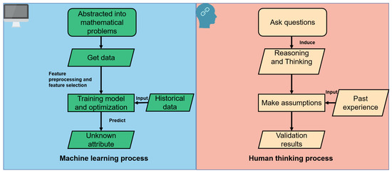
Figure 1.
Comparison of ML and human thought.
ML-based algorithms can be split into supervised and unsupervised learning techniques. Classification and regression typically involve supervised learning, which modifies the classifier’s parameters to achieve the desired performance using a set of samples from known categories. From the labeled training data, we infer a function. Unsupervised learning establishes associations between them by using categorized data [21]. We discover the model using the unlabeled data and describe the category, transformation, or probability of the data using data that was collected organically. Compressing data is the essential tenet. We may also receive semi-supervised and reinforcement learning methods by using the maximum likelihood algorithm by various training methods. To address the issue of insufficient labeled data, the semi-supervised learning method uses a large number of unlabeled samples and a small number of labeled samples. Reinforcement learning differs from the first three approaches in that feedback cannot be received right away during training, and the input is sequential data that does not satisfy the independent distribution. Agents can benefit from reinforcement learning by developing techniques to help them interact with complex surroundings to their fullest potential. Transfer learning is another teaching strategy applied in ML. The term “transfer learning” describes how one type of learning affects another type of learning or how the experience gained through learning might affect how well one completes other tasks.
Many researchers have debugged and improved ML algorithms, which have been widely utilized in classification and prediction issues and have demonstrated great performance in a variety of disciplines. Based on a classification of different ML algorithms, we examine how various ML techniques might be used to network feature measurement in this article. In Table 1, we outline the uses and performance evaluation of these algorithms.

Table 1.
Application of Network Measurement and analysis of ML algorithms.
2.1. Supervised Learning in Network Measurement
In the process of supervised learning, input data are mapped to tags, prediction models are trained using data and their matching tags, and networks are trained using known examples. Depending on the quantity of annotated training data available [32], supervised learning is frequently employed in applications such as spam detection, facial recognition, and text classification. The objective is to increase the model’s capacity for generalization in a particular area. Algorithms for classification and regression are examples of supervised learning techniques. The regression process produces continuous data, whereas the classification technique produces discrete data. The classification algorithm’s objective is to categorize the data in the set, and the regression algorithm’s objective is to find the best fitting line between these data so that every point in the dataset can be as closely related to it as possible.
The regression algorithm is one of the simplest and most common machine learning algorithms. One of the simplest and most used machine learning algorithms is regression [33] and the assessment index used in this mathematical technique for performing the predictive analysis is the discrepancy between the expected and actual values. To calculate the network quality of service, we used the return to estimate the packet loss rate and other network properties. Additionally, the distinctive correlations between application KPIs and network indicators can be inferred using multiple linear returns [34]. This study focuses on the use of classification algorithms in network measurement because there are few studies on the use of regression techniques in network measurement. The classification algorithm’s job is to classify samples into relevant groups based on those groups’ traits. The most popular classification algorithms include Bayes, ANN, decision trees, linear regression, and decision trees.
2.1.1. Random Forest in Network Measurement
Regression and classification issues are solved using RF, an integrated learning strategy. A machine learning technique called ensemble learning increases accuracy by combining various models to address the same issue [35,36]. The fundamental concept is to translate problems, such as delay prediction, into many classification labels by using multiple decision trees to merge numerous weak classifiers to get better results than simple addition. To ensure that the sample features and output outcomes of each tree are distinct, choose a portion of the samples from the training data and randomly choose some of the features for training. Random forest, as an integrated technique, fits several decision tree classifiers concurrently on various dataset subsamples and employs majority voting or averaging for the outcome. As a result, the overfitting issue can be reduced, and prediction accuracy, control, and training speed can all be improved [37]. It applies to scenes with low real-time performance requirements.
A classifier with a fair amount of accuracy, random forest can be used in a variety of situations. Giannakou et al. [38] built a simple machine learning technique based on random forest regression that can identify the minimal set of the path and host measurements needed to produce reliable and accurate predictions. The program requires very little training time and can estimate packet retransmission accurately for any quantity of data transmission. However, the issue of abnormal packet loss remains unresolved, and the random forest approach also places restrictions on the flexibility of the input parameters. As a result, changes in the input characteristics have a major impact on the predictor’s accuracy. Random forests are ensemble models that are learner-based and have low variance and bias. They can be used for classification and regression. However, when there are too many data dimensions, each value is impurely calculated, which slows down the efficiency of avoiding basic decision trees and prevents continuous output.
2.1.2. ANN in Network Measurement
An ANN is made up of a lot of connected processing units. The network processes information by progressively altering and increasing the weights of the neuron connections to replicate the relationship between the input and output through repeated learning and training of known information. Each neuron and its connection can only represent a portion of the information in an artificial neural network, which can imitate the complex nonlinear relationship well. Therefore, when there is a node break, the overall operation effect of the subnetwork is not affected, and it has strong robustness and fault tolerance. As a result, the subnetwork has excellent robustness and fault tolerance, and when a node breaks, the influence on its overall operation is unaffected. One branch of machine learning techniques, ANN, has frequently been employed in future prediction and image recognition processing due to its self-learning function, high-speed search for optimal solutions, and simultaneous processing of enormous volumes of data, addressing classification and regression issues [39].
To anticipate the possible throughput in a non-independent 5g network based on network slices, Minovski et al. [24] suggested a non-network intrusive ML model. To comprehend the decision-making procedure of root cause analysis, a decision tree model was employed. Verification yielded an accuracy rate of 93% using an ANN as the optimal method for processing the tabular dataset. An ANN has the abilities of self-adaptation, self-organization, and real-time learning and can carry out a huge number of operations quickly as a parallel and distributed processing approach. The failure to guarantee a superior effect and total reliability, however, results from extensive training and data renewal, which is unsuitable for high-precision computations.
2.1.3. SVM in Network Measurement
SVM is a collection of supervised machine learning models with nonlinear classification (SVC) and correlation kernels for regression (SVR) [40]. This approach, nevertheless, was simple and reliable. The kernel approach is used to perform nonlinear classification. As a common kernel learning method, the computational objective of SVM, a popular kernel learning technique, is to create the optimal selection or line restrictions that can divide the n-dimensional space into classes so that we can insert new information points into the appropriate classification without overstretching. The hyperplane is the name given to this optimal choice limit [41]. SVM maps the sample vector to the high-bit space, represents each sample data point in the space to distinguish distinct sample points as much as possible, and identifies the hyperplane that best separates the two types of data to maximize the distance between each classification and the hyperplane. The SVM’s classification error decreases as the distance increases. The SVM is frequently employed in binary classification issues because of its strong classification capabilities.
Mirza et al. [42] proposed a throughput estimation tool based on a support vector machine that forecasts end-to-end throughput using several stream-level features as input. The measurement accuracy, when paired with the prior file transfer and basic path attributes, was nearly three times greater than it was with the history-based method. This tool has not been validated in a big flow and scientific traffic environment; instead, it has only been evaluated on an artificial network track, taking only the unique network path into account. SVM differs from conventional statistical methods in that it essentially does not use probability measures or the law of large numbers. As a result, it considerably simplifies typical classification and regression issues. Similarly to this, utilizing SVM to deploy huge training samples is challenging. When the number is large, it takes up a lot of computer memory and processing time, and when solving the multiclassification problem, there is also the issue of classification accuracy.
2.1.4. DNN in Network Measurement
A DNN, also known as a multilayer perceptron, can be thought of as a neural network with at least one hidden layer. A feedforward neural network, or DNN, is a branch of the family of traditional artificial neural networks. Three layers make up a DNN: the input layer, the hidden layer, and the output layer. The input data are pre-processed in the layers before entering the network. In the neural network dataset, the number of input neurons is equal to the number of input features [43]. According to the general approximation theorem, a DNN relies on a large number of datasets and produces accurate and useful conclusions. In other words, by enhancing the neural network’s depth and the nonlinear effect that the activation function produces, any function can be roughly approximated. A deep neural network can be refined into scenes with uniform properties and no special reliance. It applies to any deep-learning scene.
In order to anticipate the time series of IOT traffic, Ateeq et al. [9] proposed a method based on a DNN deep neural network, and the relationship between various communication parameters and the delay was modeled. The training data’s size, depth, width, and epoch were all thoroughly examined. The prediction accuracy was then assessed using the MSE, SSE, MAE cost functions, and MAPE, with an accuracy rate of more than 98%. While modeling of DNN can more accurately and effectively depict actual complicated nonlinear issues, there are still many shortcomings in the frequency of DNN calls, data selection in the time domain, and other aspects. Layer-by-layer data pre-training, which solves the drawbacks of time-consuming and difficult manual feature designs, can be used to get the key features of each layer. Although the gradient-vanishing issue gets worse with network depth, it becomes easier for the optimization function to settle on the local optimal solution.
To determine the download and upload bandwidth measurements of the end user’s Internet connection, Maier et al. [44] employed a straightforward feedforward neural network. An artificial neural network that has been trained was used to calculate the dynamic test’s duration. The outcomes demonstrate that the dynamic duration strategy little affected the test outcomes. However, the dynamic duration test still saved a substantial quantity of data. The determined bandwidth’s deviance is disregarded. The feedforward neural network has a straightforward structure, accurately realizes any limited training sample set, and can estimate any continuous function and square-integrable function. It typically outperforms feedback networks in terms of classification and pattern recognition. The feedforward neural network has many network parameters because each layer must record the overall properties of the preceding layer. The training pace will be slow or even fail to converge when the input dimension is high.
For the time delay prediction of IOT, Abdellah et al. [27] suggested a single-step and multi-step prediction method based on a time-series NARX recurrent neural network. The RNN model was trained by adding historical data from the time series to the input layer, and until the algorithm converged, the network weight was modified by the technological error between the network prediction outputs. Three neural network training algorithms were used; MSE was chosen as the performance function to assess prediction accuracy, and RMSE and MAPE were used as the prediction accuracy indices. The Trainlm algorithm has the best prediction accuracy, and since they are neural networks with memory functions, recursive neural networks are appropriate for continuous supervised learning issues using datasets. RNN has several drawbacks as well. Recurrent neural networks must spend a lot of time intentionally labeling due to their tree structure, and the separation of each node may induce error propagation.
2.1.5. CNN in Network Measurement
To discriminate between different items in an image, CNN uses an input image and assigns importance (learnable biases and weights) to each one [45,46]. A feature extractor made up of a convolutional and pooling layer is what sets a CNN apart from a typical neural network. Only some neurons in the adjacent layer are connected to all of the neurons in the convolutional layer of a convolutional neural network. The convolutional layer of a CNN often has many feature maps. A rectangle-shaped arrangement of neurons makes up each feature map. The weight is shared by neurons with the same feature map (convolutional kernel). Sequence data processing is the main application for one-dimensional convolutional neural networks, image text recognition is the main application for two-dimensional convolutional neural networks, and medical image and video data recognition is the main application for three-dimensional convolutional neural networks.
To analyze enormous volumes of data, Sato et al. [47] devised a method for calculating the available bandwidth based on a data-driven normal form and four ML techniques. The findings indicate that CNN is the most precise method for calculating the available bandwidth. The microscopic and macro aspects of queuing delay are used by CNN to calculate the precise amount of bandwidth that is available. Two fully connected layers, two pairs of convolutional and pooling layers, and a six-layer CNN were created to estimate bandwidth. A CNN can automatically extract features since it shares the convolution kernel, which relieves the processing burden when working with high-dimensional data. The use of BP propagation to change parameters will, however, impede the change in parameters near the input layer when the network level is too deep. By neglecting the correlation between the local and the overall, the pooling layer will easily cause the training results to converge to the local minimum rather than the global minimum when the gradient descent algorithm is used.
2.1.6. LSTM in Network Measurement
An enhanced recurrent neural network called LSTM can address the RNN’s inability to handle long-distance reliance. LSTM uses a gated technique to address the issue of exploding and disappearing gradients. Since their debut, LSTMs have drawn a lot of attention for their adaptability and efficiency across a wide range of applications [48,49]. LSTM contains more parameters that can better regulate which memories are kept and which memories are destroyed at a certain time step compared to RNN, which only maintains a single hidden state. Unit state, hidden state, input gate, forget gate, and output gate are the five essential components of an LSTM. A one-step prediction with a specific reference value for time-series prediction can also be made by LSTM in addition to learning a lengthy series.
Botta et al. [23] suggested using a machine learning-based automated decision system to substitute professional users in bandwidth estimation. It is separated into the categorization system and the LSTM system. For the LSTM system, a composite dataset made up of several jobs was produced. While the second is trained simply using a bandwidth sequence, the first has many features. The performance of the LSTM system with just bandwidth was shown to be marginally superior to the performance of the LSTM system with numerous features. It outperforms the other models and is widely utilized in numerous sequence problems, including forecasting natural gas load. Parallel processing, however, also has several drawbacks. Even longer sequences still struggle with gradient loss. The LSTM neural network’s intricacy meant that training took longer than it did for CNN.
2.1.7. DT in Network Measurement
One of the most well-known techniques for representing data classification is the use of decision trees [50]. The decision tree’s non-leaf nodes have two branches that are classified as true or false. The leaf node can make decisions. Any input coming from the root node will always reach a leaf node or be the only input to do so. Based on the idea of minimizing the loss function using training data, the decision tree model was developed as a classification and regression technique. You can think of every route leading from the root node to the leaf node as a rule. The leaf node refers to the conclusion of the rule, whereas each internal node represents a condition. These rules, which are mutually exclusive and comprehensive, are applicable in situations when there are more than two realistic options that the decision-maker can select and more than two uncontrollable unknown circumstances.
Hu et al. [25] created a decision tree that just requires a modest set of features to be collected to forecast the RTT between IP pairs that are separated geographically by great distances. Based on the combination of the mutual information gain of various qualities and the RTT, a decision tree of the RTT is built. The learning process made use of several attributes. Tests of the chosen attributes are represented by the internal nodes of the decision tree. From the matching node used for attribute classification, each branch descended. The RTT level is represented by the leaf node. When the decision tree has a defined structure, a strict protocol, and a clear aim that the decision-maker expects to attain, the method can be used in large-scale systems. It enables the decision-maker to compute the gains or losses of various schemes under various conditions and estimate the likelihood of the occurrence of uncertain factors. A decision tree struggles to forecast continuous fields, though. When processing data with strong feature correlation, speed suffers and errors may multiply more quickly when there are many categories.
2.1.8. RBF Neural Network in Network Measurement
An RBF is used in the creation of an RBF neural network, which is a typical three-layer feedforward network. It can be applied to classify patterns and approximate functions. The RBF neural network has a simple structure, quick learning speed, excellent approximation, and excellent generalization ability when compared to other artificial neural networks. The RBF neural network works on the idea that the input vector can be directly transferred to the hidden space without the need for a weight connection by using RBF as the “base” of the hidden unit to build the hidden layer space. When the mapping relationship’s center point is established, the mapping relationship itself is established.
Ojo et al. [21] constructed radial basis function neural network and maximum likelihood probability neural network path loss prediction models, taking into account multi-transmitter scenarios and evaluating them. They also added a radial basis function neural network to an efficient path loss prediction. The projected path loss is the most recent measured value with a minimal error, and the RBF neural network’s prediction impact is superior to that of the MLP neural network. RBF neural networks can map any complex nonlinear connection, and they have simple learning principles, making them practical for computer implementation. They also have good nonlinear fitting capabilities. It has excellent memory, robustness, and self-learning capabilities. However, the incapacity of RBF neural networks to describe the basis and process of reasoning is one of their most critical issues. The neural network cannot operate RBF to convert all problem characteristics into numbers and all reasoning into calculations when the data are insufficient. There must have been data loss in the outcomes.
2.1.9. Discussion on Supervised Learning in Network Measurement
The performance of frequently used supervised learning techniques is listed in Table 2 based on the research in this paper. Practically speaking, classification problems have more application opportunities than regression problems, and different parts of network assessment have been addressed through the use of random forests, SVM, ANN, and FNN. Though several feature extraction techniques and datasets have been utilized by researchers, more relevant techniques have maintained a high accuracy of more than 90%. Additionally, the best answers varied depending on the various conditions. The complexity of the dataset, feature extraction, user needs, and other aspects should be taken into account while choosing an acceptable approach.
Table 2.
Network Measurement Application and ML Algorithm AnalysisPrediction accuracy of different supervised ML algorithms.
2.2. Unsupervised Learning in Network Measurement
Unsupervised clustering methods were researched before the development of deep learning and are still in use today [54]. In the real world or a real network environment, it could be difficult or expensive to manually label some data due to a lack of appropriate prior knowledge or because it would be too expensive. Unsupervised learning is now a technique used by computers to solve various pattern recognition issues based on training samples of unknown categories. It does not process supervised signals; it merely processes the so-called “features”. Unsupervised learning is used to train models to learn the structure of datasets, give users useful information about new samples, and assist managers in making the best decisions possible using both qualitative and quantitative methods. This process calls for a methodical learning process that represents precise input signals in a way that reveals the structure of the entire set of input signals [55].
The unsupervised learning algorithm has three main characteristics:
- Unsupervised learning has no clear purpose;
- Unsupervised learning does not need to label data;
- Unsupervised learning cannot quantify the effect.
Therefore, it is difficult to determine whether a job has been finished during unsupervised learning using this strategy. Unsupervised learning lacks definite markers that can be used to determine whether a goal has been attained. Currently, clustering and dimension reduction are two widely utilized unsupervised algorithms that are mostly used in the following scenarios:
- One of the most common tasks in unsupervised learning is clustering. Instead of defining groups before seeing data, it enables us to identify and evaluate naturally generated groups, that is, groups that were established depending on the data itself. K-Means, hierarchical, and probabilistic clustering are popular methods;
- Too many features could waste an ML model’s storage space and processing time in the event of a dimensional catastrophe. Researchers want to represent data accurately in smaller dimensions without sacrificing too much useful information. The dimensions of the data can be decreased using a dimension-reduction technique. PCA and SVD were the two basic methods employed.
K-Means in Network Measurement
When the datasets are segregated from one another, K-Means is a quick, reliable, and simple algorithm that can produce accurate results. This algorithm groups data points into clusters to minimize the square distance between each data point and the center of mass [19,56]. Its major job is to automatically group samples that are similar into categories. The key concept is to randomly select K objects to serve as the initial cluster centers, divide the data into K groups, measure the distance between each seed cluster center and each item, and then assign each object to the cluster center that is closest to it. Up until the termination condition was met, this process was repeated.
Botta et al. [23] suggested a machine learning (ML)-based automatic decision system to substitute expert users. To dynamically choose the optimum device to measure the available bandwidth, four ML algorithms were utilized. The CPU, memory, and bandwidth were only a few of the various parameters that were used to validate the decision system. The K-Means approach may typically be used on continuous datasets with tiny dimensions and values since it is trained by including its features in the input. It can be applied in a variety of situations, including document classifiers, item transmission optimization, and customer classification. The K-Means algorithm can perform a preliminary examination of the data and even identify the hidden value after suitable pre-processing. However, it might be challenging to understand how to choose the K-value for the K-Means technique, and it struggles to converge for non-convex datasets. Using an iterative approach, only a locally optimal solution could be found.
2.3. Reinforcement Learning in Network Measurement
The challenge of agents employing learning methods to maximize gains or attain particular objectives while interacting with the environment is described and solved using one of the concepts and methodologies of reinforcement learning. The labeling of training data is not necessary for reinforcement learning, but each action environment’s feedback must be either a reward or punishment. Feedback can be measured and given to the item to modify its behavior continuously. Trial and error is a hallmark of reinforcement learning, and time and delayed feedback are significant components. The data in supervised and semi-supervised learning are unrelated to one another and have no association. However, with reinforcement learning, this is not the case. The future receipt depends on the current situation and the decisions made. The two sets of data were correlated with one another. In the process of learning, known as reinforcement learning, agents regularly make decisions, monitor the outcomes, and then automatically modify their techniques to attain the best possible outcome. Even though this learning process is convergent, it still takes a long time to arrive at the best strategy because it must explore and learn about the entire system, making it unsuitable for large-scale networks. As a result, reinforcement learning’s practical application is quite limited [57].
The environment, state, action, and reward are also included in reinforcement learning, with the agent serving as its core component. One premise governs the reinforcement-learning training procedure. We think the entire procedure complies with the Markov decision-making procedure. The fundamental tenet is that the next state is only connected to the present state by the action that the present state must perform and only by one step. We can only easily deduce the next state from the current state and the action that has to be taken when it adheres to the MDP. During the training phase, it was convenient to infer the state change in each step. We cannot train if we are unable to deduce the state change at each stage of the training procedure. The three primary types of reinforcement algorithms are Value-Based, Policy-Based, and Actor-Critic.
Khangura et al. [28] developed single-state Dobby bandit technology using reinforcement learning and the greedy algorithm to determine the available bandwidth. The reward function was maximized to calculate the available bandwidth. Under many challenging circumstances, it converges to the available bandwidth, has a more precise estimation and a faster convergence speed in several network scenarios, and does not require noise statistics. Utilizing the exploratory development mechanism, one can learn through untrained observation of the environment while also maximizing the cumulative return function. The method based on reinforcement learning has less variability and can also get an accurate estimate of the bandwidth available. Because we frequently run into issues when using reinforcement learning for practice training, the use of reinforcement learning in network measurement is less common. The reinforcement learning sample period is excessively long, which makes it challenging to use in practice. It is easy to fall into a locally optimal solution since incentive functions are challenging to build and balance between exploration and utilization.
2.4. Transfer Learning in Network Measurement
Learning a task’s model and applying it to other tasks that are related is referred to as transfer learning, and the basis of transfer is the requirement that two learning activities be connected [58]. In other words, we can apply the lessons we choose to learn in one situation to another. A model must be built for transfer learning and then turned into a feature extraction module. The model is then applied immediately to a different task after being trained on a comparable task. The model can be fine-tuned to a new task after training so that it can more easily adapt to the new activity. Transfer learning is comparable to mimicking how the human brain thinks, in other words. If we can solve one problem, we can solve others that are related to it more effectively and quickly. Transfer learning is given a source domain and a source task, a target domain, and a target task. When the source domain or source task is not the same as the target domain or the target task, the purpose of transfer learning is to use the knowledge of the source domain and source task to enhance the prediction of the target task learning function. The definition of transfer learning, domain data, and transfer methods are only a few of the criteria that can be used to categorize transfer learning.
Transfer learning is frequently used in a variety of contexts. Transfer learning is an option if the issue falls inside the scenario. Nunes et al. [31] thought that without real measurements, network delays could be correctly anticipated. They used datasets to train the model, freeze the CNN layer of the predictor, and load out-of-date weights when data were entered. The network delay predictor was used in the real world with 93% accuracy thanks to transfer learning in an upgraded model of ML-assisted transfer learning that was built in the lab. The main problems of transfer learning are data-adaptive distribution, feature selection, and subspace learning, and it is demonstrated that transfer learning is superior to begining from scratch in terms of both accuracy and training time. It can address issues with a variety of duties, fewer data in the new office, and differing data distributions between the new office and the old office. The transfer cannot be used if there is no connection between the source and target domains. In the worst circumstances, this interferes with the target field’s task learning. Negative transfer is a circumstance that needs to be avoided as much as feasible.
2.5. Semi-Supervised Learning in Network Measurement
Unsupervised and supervised learning are combined in semi-supervised learning. It performs pattern recognition using both labeled and a sizable amount of unlabeled data. In practice, there are far more unlabeled training samples than labeled training samples. In this situation, where untagged data are easily accessible, and tagged instances are frequently challenging, expensive, and time-consuming, the SSL technique is better suitable for real-world applications. To make up for the lack of markup training data, SSL can create superior classifiers [59].
There are still some flaws in the theory that semi-supervised learning has proposed because it has only recently been developed. Three reliability-related presumptions are made, and they are as follows: Semi-supervised learning depends on relative simplicity, and data processing does not account for noise interference to samples, which is unavoidable in real life. Additionally, semi-supervised learning is unable to pinpoint the conditions under which the classification performance of unlabeled data can be enhanced. Semi-supervised learning performs worse than supervised learning when the model or parameters are incorrectly chosen. As a result, semi-supervised learning is currently primarily experimental on synthetic datasets, and further study is necessary before it can be applied to real datasets. As a result, network measurement has not yet used semi-supervised learning.
2.6. Discussion of Different ML Methods in Network Measurement
We introduce the application of supervised learning, unsupervised learning, reinforcement learning, and transfer learning to network measurements in the second section. The aforementioned findings demonstrate that most datasets in the field of network measurement contains labeled data. Hence most researchers still opt for supervised methods to teach and train their models. In terms of network metrics, supervised learning has developed and is at a good level of development. In comparison to other learning algorithms, including unsupervised learning, it is popular and performs well. Advanced training data are not necessary for unsupervised learning. A dataset can be directly modeled. Unsupervised learning’s main goals are to train the model that will be used to learn the dataset’s structure and to give users meaningful knowledge about fresh samples. As a result, all we need to do to apply the clustering algorithm to get the desired outcomes is to understand how to calculate data similarity. Semi-supervised learning has not been used for network measurement compared to supervised and unsupervised learning due to its rapid development and scant theoretical backing. Both reinforcement learning and transfer learning are now in use; however, due to the differences between the two learning techniques, few academics are interested in them. In conclusion, supervised learning is currently the most widely used technique for measuring networks, which is consistent with tendencies in future development.
3. Network Measurement Based on ML Method
According to the classification of ML methods, which is the subject of this study, the application of various ML approaches to network measurement is introduced in the second section. Understanding the key traits of the various ML algorithms is useful for researchers. This section of the article will provide the ML-based solution from the standpoint of a real-world network measurement application. To characterize and visualize network behavior and quantify numerous network indicators, network measurement’s primary objective is to gather traffic data linked to network operation [60]. According to the classification standard for network measurement objects, network measurement can be further separated into active measurement, passive measurement, network performance measurement, and network traffic measurement. An ML technique based on a network measurement object is presented in this study. Measurements of latency, packet loss, path loss, throughput, and bandwidth are all examples of network performance metrics. As demonstrated in Table 3, this article provides a detailed introduction to various application situations utilizing the ML approach for network monitoring.
3.1. Network Delay and RTT
Network performance measurement is now essential for identifying the root causes of network performance degradation due to the growth in network complexity and scale. A key metric of network performance is packet latency. The accurate measurement of the time delay or its distribution is the current emphasis of time-delay measurement. The amount of data required for the delay measurement may be enormous in an actual network because the measurement may extend for several days, weeks, or even longer. Therefore, a constant issue in the delay measurement is the quick processing of these enormous and high-latitude data. Low latency can enhance service quality, particularly for applications that require quick response times. To address network delays, it is crucial to significantly enhance algorithm selection, modification, and prediction capabilities [61,62]. Additionally, there is a concern with the lack of testing for network-link congestion or large-scale file transmission in the existing review procedure.
Among all the features that might be utilized for the experiment, an ML technique was proposed that employs a random forest approach to choose RTT as the most crucial attribute. Several decision trees were then used to assign labels to each input record. This considerably reduces the amount of data (by more than 60%) by minimizing the information loss of the prediction RTT. Guo et al. [63] suggested a path delay change prediction model based on random forest and BP neural networks. Based on the prepared path for the network configuration, the fundamental path features were retrieved. Both the computational work for the interpolation method of non-grid timing and the work characterizing the timing database of each cell has been left out. It can more accurately forecast the change in path delay under a curve that was not simulated when the training set was being created.
In their papers, Nunes et al. [31,64] provided a precise estimate of the TCP round-trip time using ML technology known as the expert framework. The “experts” all provided fixed value estimates. The RTT is the weighted average of these estimates, and the weight is adjusted after each measurement of the RTT by the discrepancy between the estimated and real RTT. The latter employs a retransmission timeout timer, which incorporates TCP error and congestion control but does not routinely assess RTT. Throughput increased while the quantity of retransmitted packets drastically dropped. To forecast the IOT delay, Abdellah et al. [65] employed the maximum likelihood approach based on the NARX recurrent neural network. MSP and single-step prediction are the two time-series prediction techniques that were suggested. Embracing the root means square error and the lowest root mean square error helped gauge the accuracy of the predictions. An ANN was used to examine the prediction of packet transmission latency in a self-organizing network.
3.2. Packet Loss
The term “packet loss” refers to the failure of one or more packets’ data to travel through a network to their intended location. Numerous factors contribute to this, including packet loss due to channel blocking at the early layer and signal attenuation brought on by multipath fading on the network. The quality of multimedia applications that depend on delay is largely determined by packet loss [66]. Some applications in scientific networks demand frequent, large-volume data transfers with precise network performance specifications; as a result, transmission becomes extremely sensitive to performance deterioration events [22]. Keeping track of packet loss on a link enhances network administration and service [67]. Thus, to enable researchers or network operators to reduce packet loss through various host or stream reallocation technologies, advanced technologies are needed. Due to this requirement, researchers started to forecast packet loss using ML techniques.
To forecast the packet loss rate, Roy et al. [22] employed a decision tree and a logical regression model. To present decisions and potential outcomes, a decision tree was employed as a tool. To conduct predictive analysis and characterize the data, logical regression was utilized. The decision tree approach, in comparison, has a stronger predictive impact. For the IoT’s packet loss prediction, Abdellah et al. [65] suggested a multi-step advance prediction time series based on a feedback neural network. However, because packet loss and queuing delay are closely related and because most researchers still focus on queuing delay, there is little research on the packet loss rate. Instead, the prediction accuracy of the neural network learning process is estimated by the mean square error, maximum likelihood error, and minimum mean square error. The issue of unusual packet loss instances is still open. The chosen method places restrictions on the flexibility of the output and input parameters, and data delivery without retransmission is unpredictable. Changes in the distribution of the input characteristics had a major impact on the forecast period’s accuracy as well.
3.3. Throughput
Throughput, which is a key metric of network performance, is the quantity of data successfully transmitted per unit of time for networks, devices, ports, and other facilities. The internal and external network interface hardware of the network equipment, as well as the effectiveness of the program algorithm, especially the program algorithm, are the key determinants of throughput. The best throughput method is one which, for a certain TCP transmission size, can be accomplished via a particular path between two end hosts. Creating a solution that accurately predicts TCP performance for arbitrary and potentially highly dynamic end-to-end links is the fundamental difficulty [42].
Mirza et al. [42] generated throughput estimations by using SVR’s ability to take various inputs. The actual throughput of the target TCP stream was measured on-site in comparison to the predicted throughput produced by numerous instances of our SVR-based algorithms that were trained using various combinations of path parameters. Throughput prediction can increase by up to three times when path attributes are taken into account using SVR-based tools in comparison to history-based predictors. Lazaris et al. [68] provided a paradigm for deep neural network-based traffic-based throughput classification. Using t-distribution random neighbor embedding, it presents a real dataset of 252 million traffic records amassed in a single week (t-SNE). Instead of dividing the expected bit rate into elephant and mouse flows, their objective was to divide it into three categories. The number of nodes, number of layers, and learning rate were three super parameters that were optimized. The results of the trial revealed that during a continuous period of one week, the prediction’s accuracy averaged 82%. As a benchmark, Minovski et al. [24] measured the throughput of each network slice’s cellular links. He then utilized the DTs model to better understand how root cause analysis decisions are made. The chosen method for processing tabular datasets, particularly an MLP, is an ANN. To forecast the available throughput in a non-independent 5G network based on network slices, a non-network intrusive machine learning approach is suggested. To predict the link throughput using a real traffic dataset, Chen et al. [69] evaluated the effectiveness of the LSTM network and ARIMA model. For the test split, they assessed the duration of four epochs and three iterations of each model. In each instance, the LSTM network’s average error was much lower than the ARIMA model’s average error. Currently, the majority of studies using machine learning to estimate throughput only analyze the artificial network path, only taking into account the particular network path, and have not been tested in a big flow and scientific traffic environment.
3.4. Bandwidth
The amount of data that may be transmitted in a given length of time is referred to as network bandwidth. The fundamental element of digital communication, particularly in packet networks, is bandwidth, which refers to the quantity of data that can be carried in a given length of time through links or network channels. The three indicators, capacity, available bandwidth, and batch transmission capacity, are all measured by existing bandwidth estimate techniques. When transmitting data, a reliable bandwidth should ensure that there is no congestion and that it can be cleared quickly by predetermined standards [70]. The statistical cross-flow model and the self-induced congestion model, two frequently used bandwidth assessment techniques, now have issues. When the network scenario is complex, there may be inaccuracy or behavioral interference. To assess the bandwidth of Internet links, new techniques must be used. The majority of academics now favor ML.
Chen et al. [29] suggested a system for anticipating traffic bandwidth. A support vector machine can interpolate or extrapolate the system output based on the characteristics of the test input, even if the system output is not present in the training dataset. A support vector machine also has a reasonable computational cost. A simulation was used to determine the available bandwidth. In all test instances, the results demonstrate that the pathChirp model is superior to the package sequence model. Additionally, this approach has more precise estimates than the two widely used tools, pathChirp and Spruce, by combining the pathChirp-like model with an SVM. The original dichotomy approach was replaced by a neural network by Khangura et al. [71] to decide the next detection rate, and the available bandwidth was calculated using the information already present in the program between them. To forecast the output bandwidth and an input vector that is not filled up, two neural networks were trained.
To reduce prediction difficulty, Khangura et al. [28] simplified the prediction problem of the actual available bandwidth into a classification problem. The prediction results were filtered through training with fewer data. A k-dimensional vector was used as the input. The process was, detect, collect relevant information, combine them into a complete k-dimensional vector, and then input them into the classifier. The SVM, K-NN, AddBoost, and other ML methods were selected. The range to which the actual available bandwidth belongs is the output, and the midpoint of the range is set as the estimated value; median filtering was applied to the estimated values to improve the accuracy. Hága et al. [30] unveiled a neural network-based empirical bandwidth estimation tool. The neural network was trained using simulation data, and it is capable of accurately estimating the physical and available bandwidth for single-hop and multi-hop networks in both the lab setting and under real-world settings on the ETOMIC test bench. It has been established that the input data are the only factor limiting the accuracy of bandwidth estimates. Other network analysis issues can simply be addressed using this approach. Khangura et al. [72] trained the packet dispersion vector as a characteristic of the available bandwidth using a neural network. To choose the next detection rate, an iterative neural network rather than a binary search approach was suggested. The issue of estimating the available bandwidth was described as a classification challenge. The suggested method is assessed using support vector regression, Gaussian process regression, and random forest. The findings demonstrate that by lowering the bias and variability, the neural network may greatly enhance the estimation of the available bandwidth. Labonne et al. [73] evaluated three machine-learning techniques to forecast bandwidth usage 15 seconds in advance. Network link use can be predicted using LSTM models with good accuracy (the error is less than 3%).
The degree of improvement varies depending on the position of the filling elements, the number of existing elements, and the position of the existing elements in some approaches that only use a small number of detection rates. Overfitting occurs when there is insufficient data for training. Because each class defines a real number range, errors will still occur even if the classifier classifies the data correctly. The maximum error happens when the available bandwidth is at the class’s edge. The actual bandwidth can be converged by direct detection techniques. It cannot, however, keep up with rapid fluctuations in bandwidth. While reducing probe traffic helps to estimate the available bandwidth, it also causes network congestion. With more links, the misclassification error rose, necessitating additional training data.
3.5. Path Loss
The loss brought on by the spread of radio waves through space is referred to as path loss. The channel’s propagation characteristics and the radiation diffusion of the transmission power are to blame for this. This indicates the shift in the signals’ average power at the macroscale. The strength of the received signal is greatly impacted by obstructions in the signal route between the transmitter and receiver in a wireless propagation scenario. Path loss describes the attenuation of this signal strength. Planning, optimization, and interference analysis for networks all depend on precise path loss characterization and modeling. Several path loss prediction algorithms have been put forth recently to enhance network performance. Implementing a single-path loss prediction model that is appropriate for all wireless propagation conditions, however, is a basic issue that the majority of these models fail to address [8]. That is to say, ML can give a flexible network topology and can use a lot of data to increase the accuracy and performance of signal prediction. People start looking for new ways to overcome these difficulties.
Ostlin et al. [74] suggested and assessed a model for an artificial neural network to predict macrocell path loss. We examined neural networks of various sizes from multilayer FNN neural models. To improve prediction accuracy and generalization properties while shortening training time, a quicker training algorithm was incorporated into the training process. Popoola et al. [75] developed an optimization model for path loss using a feedforward neural network technique. With the help of normalized terrain profile data and normalized distance, a single-layer fuzzy neural network was trained to calculate the corresponding path loss value using the Lvenberg Marquardt algorithm. By varying the number of hidden layer neurons, the ANN with the best prediction accuracy was found. Ojo et al. [76] predicted path loss in a research environment using radial basis function and support vector regression. The SVR and RBF ML algorithms’ precise system architecture was optimized by adjusting the hyperparameters of the RBF model. Five other empirical models’ performance was compared to that of SVR and RBF ML, and it was found that the ML models’ performance was superior to those of the empirical models. In order to provide a resilient network structure, robust adaptability, and wide-ranging data availability, the ML algorithm was applied to signal propagation modeling. Many components, from the transmitter to the receiver, can be accurately modeled using ML for signal propagation. However, researchers have discovered that more sophisticated neural networks might not be more effective, and larger FNN might provide erroneous predictions as a result of overtraining. In addition, rather than overcorrecting and overpredicting, more focus should be placed on carefully choosing training data and broader datasets.
3.6. Congestion Control
The load of the communication network has a direct impact on the throughput of the network. If the throughput drops when the network load reaches a specific level, congestion develops. When congestion is severe, it will cause wasteful retransmissions, which will lower the communication subnet’s effective throughput and eventually push the local or even all communication subnets into a state of deadlock, with an effective network throughput that is near zero. In the present situation, congestion detection in wireless sensor networks is a significant issue. Currently, several academics employ machine learning techniques to identify congestion.
Singhal et al. [77] identified congestion in the transport-layer sink node using an NN-based congestion detection method. The output was the degree of congestion, while the input parameters were the number of participants, buffer occupancy, and traffic. Numerous simulation results demonstrate the scheme’s ability to detect and better reflect the level of congestion in sensor networks. Madalgi et al. [78] created a congestion detection classifier with three levels: low, middle, and high using an open-source SVM package and a sequence-to-minimum optimization approach. When the radial basis function is chosen as the kernel-function model, gamma and cost are crucial factors to consider. By modifying various factors, the ideal model training time can be achieved. Scholars generally agree that M5 decision trees are superior to general NN and that employing neural networks to predict network congestion is better than empirical models after analyzing various studies.
3.7. Discussion on Network Measurement Application with ML
Six facets of network measurement using the ML approach are discussed in the third section. Network measurements can gather information about network operations’ traffic and use it to inform all facets of network operations. The ML approach effectively extracts valuable network features, classifies and predicts the desired information we want to know, and manages network features as necessary. In recent years, network measurement has gained popularity as a study area. Especially when network bandwidth is expanding, it offers a smart control approach for future efficient and high-quality network transmission. Currently, throughput, delay, and available bandwidth are all addressed by the ML technique. We are aware that these three can interact with one another in some ways, and Figure 2 shows how they relate to one another. Additionally, a network’s utilization rate is extremely high if throughput is virtually equal to bandwidth. The bandwidth problem is, in some ways, simpler to fix than the latency issue.
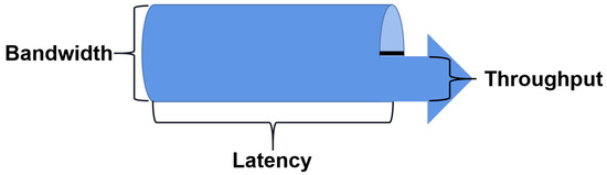
Figure 2.
Throughput, bandwidth, and delay.
Therefore, to aid networks in achieving more efficiency, the majority of scholars have concentrated on gaining more available bandwidth and producing more precise estimates of the available bandwidth. As opposed to the conventional empirical model of traffic measurement, the ML method can convert the detection of abnormal behaviors into pattern recognition when they occur in a network. It then classifies these behaviors by examining the characteristics of network traffic and the data gathered to differentiate between normal and abnormal behaviors. Because of the significant labor time savings, the ML approach has drawn increased attention. The study’s findings demonstrate that, despite the possibility that the best suitable machine learning techniques vary depending on the circumstances, the use of ML in network assessment has advanced significantly and quickly. The public will see more and more appropriate general models as software and hardware development continues, in addition to the optimization of various models and the adjusting of datasets.
Table 3.
Network Measurement Application and ML Algorithm Performance Analysis.
Table 3.
Network Measurement Application and ML Algorithm Performance Analysis.
| Scenarios | Applications | Ref | ML Algorithms | Performance Analysis |
|---|---|---|---|---|
| Path delay | Reduce data volume | [51] | RF, LR, SVM | It shows the importance of data pre-evaluation and feature selection, but the basic algorithm can not provide high accuracy in this case. |
| Reduce computing effort | [79] | RF, BP NN | It can better predict the change in path delay under the curve that has not been simulated during the preparation of the training set. | |
| Provides accurate estimation of round-trip time in TCP transmission | [31,64] | Experts Frame | The number of retransmitted packets decreases significantly, and the throughput increases. | |
| Predicting Delay in IoT Models | [80] | RNN, ANN | Compared with similar models, the model using the Trainlm training algorithm has the best prediction accuracy, while the model using the Trainrp training algorithm has the lowest prediction accuracy. | |
| Packet loss | Faster computing with lower call latency | [65] | DT, LR | Use LR to perform predictive analysis and describe data. By contrast, the DT model has a better prediction effect. |
| Combining the two networks for prediction | [42] | ANN, RNN | Improve the accuracy of Internet of Things traffic prediction. | |
| Throughput | Use characteristics to generate throughput predictions | [24] | SVR | Use different combinations of path attributes for training. Compared with the history-based predictor, the efficiency is improved by three times. |
| Three super parameters are optimized | [69] | DNN | The prediction achieved an average accuracy of 82% over a continuous time interval of one week. | |
| Forecast based on the cellular link throughput of each network slice | [23] | DT, ANN, SVR, MLP | The non-network intrusive machine learning model is used to predict the available throughput in a non-independent 5G network based on the network slice. | |
| Evaluate three variations of each model for four epoch durations | [74] | LSTM | In each case, the average error obtained by the LSTM network is significantly lower than the ARIMA model | |
| Bandwidth | The available bandwidth is obtained through simulation | [81] | SVM | The combination of the pathChirp-like model and SVM can obtain a more accurate estimation than the two widely used tools. |
| Use the existing program information to estimate the available bandwidth | [71] | ANN | Two neural networks are trained to deal with incompletely filled input vectors and prediction of output bandwidth, respectively. | |
| Simplify the prediction of actual available bandwidth into classification | [47] | ANN, SVM, K-NN | Median filtering of estimated values to improve accuracy. | |
| Provides reliable physical and available bandwidth estimation for the simulated single-hop and multi-hop networks | [72] | ANN | It is proven that the accuracy of bandwidth estimation is only limited by the input data. | |
| The available bandwidth estimation task is described as a classification problem. | [26] | SVM, RF | Proved that neural networks can significantly improve available bandwidth estimation by reducing bias and variability. | |
| Path loss | A faster training algorithm is added to the training process | [75] | ANN | The prediction accuracy and generalization characteristics are given while reducing the training time. |
| Establish the optimization model of path loss | [76] | ANN, FNN | ANN with the highest prediction accuracy by changing the number of hidden layer neurons. | |
| Several super parameters of the RBF model are adjusted | [52] | SVM | By comparing the performance of SVR and RBF machine learning with the other five empirical models, it is concluded that the performance of the machine learning model is higher than that of the empirical model. | |
| Congestion control | Detect the congestion of the transport layer sink node | [82] | ANN | It can accurately detect the degree of congestion in wireless sensor networks and can better reflect the congestion state. |
| An effective method to determine the best parameters of classifier model selection | [53] | SVM | Improve accuracy through optimal parameters. |
4. Future Work
The future network architecture still has a lot of performance difficulties to overcome because high-speed network access is no longer an extravagance and because network demand is only expected to increase. Traditional network models and processing techniques are no longer able to satisfy people’s demands for network efficiency due to the slow pace of network innovation. A recent research hotspot, the ML approach reflects its role as a catalyst for network innovation and development. Early attempts at artificial intelligence aimed to improve the logical reasoning capabilities of machines, but as technology advanced, it became clear that this was far from enough. Some academics think that knowledge is essential for solving complicated situations more effectively. After 1980, ML emerged as a distinct field and advanced quickly. It has gradually been used in several different fields. The execution capability of the system, exemplified by Samuel’s chess program, was primarily researched in the 1950s. Hayes Roth and Winson’s systematic approach to structural learning serve as a good example of the 1960s’ goal of studying how to replicate human learning in computers. For ML, the 1970s were a time of great growth. A surge in ML research and development has resulted from the integration of learning systems with numerous particular applications using a variety of techniques and tactics. Assisted learning by Mostow is an example of his work. Several new disciplines that incorporate ML are starting to take shape. A consensus has progressively emerged on several fundamental ML and AI issues.
4.1. Future ML in Network Measurement
Many widely used methods have been generated by the development of ML. The optimum method is still defined by the dataset that researchers need to process, the data’s features, the processing goals, etc. The ML approach needed for special cases is, in a sense, specific. The requirements of a particular scenario are thus a very crucial aspect in obtaining higher performance in network measurements, and this study illustrates the abstract level of ML in Figure 3. The data preparation module, which is at the first level, consists of data selection, analysis, and pre-processing. The model is created, trained, and continuously adjusted and optimized in the second layer. The trained model is then utilized in real-world settings by task requirements.
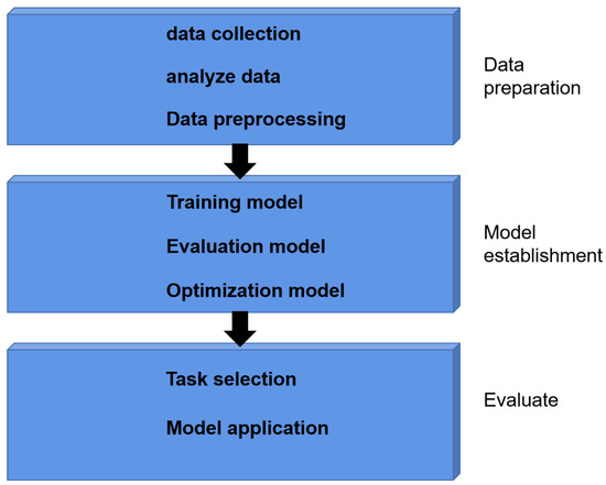
Figure 3.
Abstract hierarchy of ML.
4.1.1. Dataset
For the development of machine learning models or data-driven real-world systems, the availability of data is seen as essential [83]. Data preparation is at the lowest level of abstraction, as seen in Figure 3. High-quality data has always been the most crucial component in employing the ML approach to solve problems, regardless of the industry. The end outcome is greatly influenced by the data source and data label used. In most cases, the datasets obtained cannot be used directly in dealing with practical problems because the sample data may have issues, such as missing labels, too high dimensions, too low dimensions, and the inability to accurately distinguish between validation data and test data. If these factors are ignored, it is frequently difficult for the final result to reflect the real situation. When it comes to solving difficulties, a decent dataset can be of considerable assistance to researchers; in other words, the dataset’s quality directly affects how far the results can go. The dataset, in general, reflects the network’s overall architecture.
4.1.2. Define and Express Problems
We frequently break down real-world issues into their parts or other mathematical issues. When examining issues, it is important to identify the root causes and find remedies. Many issues with the model selection will arise from inaccurate problem analysis or poor comprehension of the problem’s purpose. Additionally, the outcomes of the flawed goal were invalid. Additionally, this study discovered that several algorithms, including SVM and RF, have good performance and versatility in terms of algorithm selection. We also discovered that neural networks, such as FNN and logical regression, may produce better results in particular cases, even though these algorithms can address the majority of the requirements. In order to explain issues to be solved as correctly as possible in mathematical language, which will become the key to the ML approach in network measurement applications, it is erroneous to pursue algorithms with strong performance mindlessly. Because ML model training takes a lot of time, setting the right goal at the outset will prevent researchers from wasting time.
4.1.3. Model Establishment and Optimization
A modeling issue was resolved once the issue was stated. The ML model was created using rules and was abstracted from the data. The model can be trained, the technology and technique can be learned from the data, different models produce different results, and applying different approaches to the same model will produce different results when the data are available after processing, and the problem is properly specified. The ML model with the best performance may not be the best option, and a successful model establishment does not guarantee a successful outcome. The model’s final findings will be impacted by concept drift, high deviation or high square error, and regularization settings. A major issue now is how to demonstrate that your model performs better than other models. The same topic may be approached by different researchers in several ways, and the optimization process is particularly important. Typically, the findings of the training model are taken into account when optimizing the model. Common techniques include choosing a better algorithm, addressing the issue of overfitting and underfitting, and optimizing super parameters.
4.1.4. Algorithm Selection
In general, comparing different algorithms can enhance model performance. For various datasets, different methods have been developed. Methods were used to implement ML, and in the sections before this one, we described how ML algorithms were used to measure networks. We cover a variety of angles on algorithm selection in this section. In order to choose an algorithm for training after creating a model without having to halt the process, we generally need to be aware of the situations and constraints of an algorithm or its powerful functions. Before selecting an algorithm, one should determine the issue that they are trying to resolve, such as when employing a recommendation system to address a particular issue. Logic regression and supervised learning can be used to create more comprehensive models or find anomalies in other open problems. The understanding of the data, the categorization of the problems, and the knowledge of the software and hardware are the primary factors that influence the choice of algorithms. Whether a high number of classification models or clustered data can be saved depends on the system’s storage capacity. Model optimization and algorithms go hand in hand, and it is frequently the case that the best method is demonstrated during this process.
4.1.5. Discussion on Future ML Methods
We list the issues that must be solved using the ML approach in this section. Although these issues appear straightforward, they can be gradually adjusted to fit the particular circumstance. A thorough comprehension of the issues that need to be resolved in ML methods will aid researchers in their work, speed up the development of ML in the field of network measurement, and increase the usability and dependability of future ML algorithms. There is yet no established optimum method to resolve this set of issues, even though many academics are researching the application of machine learning to the subject of network measurement. For the time being, the study only focuses on adapting one or more machine learning algorithms to handle certain challenges. The two main challenges for network management in the future will be how to gather a huge amount of high-dimensional data in a real network for analysis and how to create a network management system through network measurement. In general, the future will see a new stage of development in the interaction between machine learning and network measurement. Network measurement will be autonomous and intelligent thanks to the use of machine learning in picture identification, traffic prediction, and other areas. Examples of these capabilities include:
- Congestion control;
- Automatic extraction of the most important features;
- Network routing;
- Time-series analysis;
- Network layer analysis.
The ML approach is now the most successful and promising method for addressing network measurement challenges. It is supported by ML framework theory and the data of each study. ML assists decision-makers in deriving knowledge from the data and choosing the best course of action. There is no conclusive evidence that the ML approach is not practical for network measurement and that supervised learning is the most popular method for network measurement, despite the claims of certain academics that the application of ML in network measurement is still insufficient. Because supervised learning makes use of prior experience to forecast results, it aids students in altering their model of prior experience and can offer a precise grasp of the category of objects. Because unsupervised learning has no corresponding output, and the input data are not marked on the algorithm outputs; it cannot produce the desired findings that researchers are hoping to see. Due to its lengthy development process and scant conceptual underpinning, semi-supervised learning is still less common in the field of network measurement. Deep learning models are a black box, even though they are frequently employed in a variety of contexts. It is challenging to comprehend their functions, which makes it challenging to comprehend the input traits that result in these outcomes. This is one reason why deep learning’s capacity to address network issues is somewhat constrained. Reinforcement learning and transfer learning perform less well than supervised learning in some applications because of the lengthy sampling period and the fact that they are only relevant to familiar settings.
5. Conclusions
In this paper, the ML algorithm and its practical use in network measurement are discussed about the viability of using the ML approach to network measurement. This article introduces various ML algorithms used for network monitoring from the standpoint of classifying ML methods. It concentrates on using ML algorithms for network measurement, though. Most academics prefer supervised learning over other learning techniques, including unsupervised learning, semi-supervised learning, reinforcement learning, and migration learning, because of its high accuracy and the fact that the majority of datasets include labeled samples. Currently, supervised learning will continue to be a key component of future machine learning algorithms used in network monitoring. The challenges and potential possibilities for ML algorithms development in the area of network measurement are also noted. Due to the lesser complexity and expense of dealing with available bandwidth compared to some other network characteristics, the majority of research directions in the application of network measurement concentrate on this factor. Furthermore, the challenges that the ML algorithm faced when measuring networks are identified, as well as potential future study areas. The complexity of the model and the limits of the training data make it challenging to find the most efficient ML method, which is why the ML algorithm occasionally performs below expectations, even though it has made enormous strides in the field of network measurement. As network measurement using the ML method plays a significant role in future network construction and network performance improvement, including congestion control, resource management, and real-time monitoring, it is hoped that the discussion in this paper can offer straightforward assistance for scholars in related fields to apply the ML algorithm to network measurement. This will help researchers in different fields master some basic problems. The main issues raised by this study will be thoroughly investigated in the future.
Author Contributions
M.S., conceptualization, methodology, software, formal analysis, investigation, writing—original draft; B.H., investigation; R.L., investigation; J.L., supervision; X.Z., supervision; All authors have read and agreed to the published version of the manuscript.
Funding
This work was supported by the National Natural Science Foundation of China under Grant No. 92067108, the Shandong Provincial Natural Science Foundation of China under Grant No. ZR2020MF057, and the Beijing Nova Program of Science and Technology under grant Z191100001119113.
Conflicts of Interest
The authors declare no conflict of interest.
Abbreviations
The following abbreviations are used in this manuscript:
| ANN | Artificial Neural Network |
| SVM | Support Vector Machine |
| DNN | Deep Neural Network |
| DT | Decision Tree |
| FNN | Feedforward Neural Network |
| RNN | Recursive Neural Network |
| LSTM | Long Short-Term Memory |
| CNN | Convolutional Neural Networks |
| RBF | Radial Basis Function |
| XGBoost | eXtreme Gradient Boosting |
| LR | Logistic Regression |
| SVR | Support Vector Regression |
| RF | Random Forest |
| MLP NN | Multilayer Perceptron Neural Networks |
| SSL | Semi-Supervised Learning |
References
- Gheisari, M.; Alzubi, J.; Zhang, X.; Kose, U.; Saucedo, J.A.M. A new algorithm for optimization of quality of service in peer to peer wireless mesh networks. Wirel. Netw. 2020, 26, 4965–4973. [Google Scholar] [CrossRef]
- Qi, J.; Wu, F.; Li, L.; Shu, H. Artificial intelligence applications in the telecommunications industry. Expert Syst. 2007, 24, 271–291. [Google Scholar] [CrossRef]
- Feldmann, A.; Gasser, O.; Lichtblau, F.; Pujol, E.; Poese, I.; Dietzel, C.; Wagner, D.; Wichtlhuber, M.; Tapiador, J.; Vallina-Rodriguez, N.; et al. The lockdown effect: Implications of the COVID-19 pandemic on internet traffic. In Proceedings of the ACM Internet Measurement Conference, Virtual Event, 27–29 October 2020; pp. 1–18. [Google Scholar]
- Sun, Y.; Peng, M.; Zhou, Y.; Huang, Y.; Mao, S. Application of machine learning in wireless networks: Key techniques and open issues. IEEE Commun. Surv. Tutor. 2019, 21, 3072–3108. [Google Scholar] [CrossRef]
- Zhao, Y.; Li, Y.; Zhang, X.; Geng, G.; Zhang, W.; Sun, Y. A survey of networking applications applying the software defined networking concept based on machine learning. IEEE Access 2019, 7, 95397–95417. [Google Scholar] [CrossRef]
- Zhang, X.; Wang, Y.; Yang, M.; Geng, G. Toward concurrent video multicast orchestration for caching-assisted mobile networks. IEEE Trans. Veh. Technol. 2021, 70, 13205–13220. [Google Scholar] [CrossRef]
- Yao, S.; Wang, M.; Qu, Q.; Zhang, Z.; Zhang, Y.F.; Xu, K.; Xu, M. Blockchain-empowered collaborative task offloading for cloud-edge-device computing. IEEE J. Sel. Areas Commun. 2022, 40, 3485–3500. [Google Scholar] [CrossRef]
- Ojo, S.; Akkaya, M.; Sopuru, J.C. An ensemble machine learning approach for enhanced path loss predictions for 4G LTE wireless networks. Int. J. Commun. Syst. 2022, 35, e5101. [Google Scholar] [CrossRef]
- Ateeq, M.; Ishmanov, F.; Afzal, M.K.; Naeem, M. Predicting delay in IoT using deep learning: A multiparametric approach. IEEE Access 2019, 7, 62022–62031. [Google Scholar] [CrossRef]
- Shafiq, M.; Tian, Z.; Bashir, A.K.; Du, X.; Guizani, M. CorrAUC: A malicious bot-IoT traffic detection method in IoT network using machine-learning techniques. IEEE Internet Things J. 2020, 8, 3242–3254. [Google Scholar] [CrossRef]
- Park, J.; Samarakoon, S.; Bennis, M.; Debbah, M. Wireless network intelligence at the edge. Proc. IEEE 2019, 107, 2204–2239. [Google Scholar] [CrossRef]
- Tjoa, E.; Guan, C. A survey on explainable artificial intelligence (xai): Toward medical xai. IEEE Trans. Neural Networks Learn. Syst. 2020, 32, 4793–4813. [Google Scholar] [CrossRef]
- Abdellah, A.R.; Mahmood, O.A.; Kirichek, R.; Paramonov, A. Machine learning algorithm for delay prediction in IoT and pactile internet. Future Internet 2021, 13, 304. [Google Scholar] [CrossRef]
- Wang, C.X.; Di Renzo, M.; Stanczak, S.; Wang, S.; Larsson, E.G. Artificial intelligence enabled wireless networking for 5G and beyond: Recent advances and future challenges. IEEE Wirel. Commun. 2020, 27, 16–23. [Google Scholar] [CrossRef]
- Wang, M.; Cui, Y.; Wang, X.; Xiao, S.; Jiang, J. Machine learning for networking: Workflow, advances and opportunities. IEEE Netw. 2017, 32, 92–99. [Google Scholar] [CrossRef]
- Jiang, J.; Sekar, V.; Stoica, I.; Zhang, H. Unleashing the potential of data-driven networking. In Proceedings of the International Conference on Communication Systems and Networks, Bengaluru, India, 4–8 January 2017; pp. 110–126. [Google Scholar]
- Janiesch, C.; Zschech, P.; Heinrich, K. Machine learning and deep learning. Electron. Mark. 2021, 31, 685–695. [Google Scholar] [CrossRef]
- Ray, S. A quick review of machine learning algorithms. In Proceedings of the 2019 International Conference on Machine Learning, Big Data, Cloud and Parallel Computing (COMITCon), Faridabad, India, 14–16 February 2019; pp. 35–39. [Google Scholar]
- Sarker, I.H. Machine learning: Algorithms, real-world applications and research directions. SN Comput. Sci. 2021, 2, 160. [Google Scholar] [CrossRef] [PubMed]
- Sarker, I.H.; Kayes, A.; Watters, P. Effectiveness analysis of machine learning classification models for predicting personalized context-aware smartphone usage. J. Big Data 2019, 6, 57. [Google Scholar] [CrossRef]
- Ojo, S.; Imoize, A.; Alienyi, D. Radial basis function neural network path loss prediction model for LTE networks in multitransmitter signal propagation environments. Int. J. Commun. Syst. 2021, 34, e4680. [Google Scholar] [CrossRef]
- Roy, K.S.; Ghosh, T. Study of packet loss prediction using machine learning. Int. J. Mob. Commun. Netw. 2020, 11, 1–11. [Google Scholar]
- Botta, A.; Mocerino, G.E.; Cilio, S.; Ventre, G. A machine learning approach for dynamic selection of available bandwidth measurement tools. In Proceedings of the International Conference on Communications, Montreal, QC, Canada, 14–23 June 2021; pp. 1–6. [Google Scholar]
- Minovski, D.; Ogren, N.; Ahlund, C.; Mitra, K. Throughput prediction using machine learning in LTE and 5g networks. IEEE Trans. Mob. Comput. 2021, 22, 1825–1840. [Google Scholar] [CrossRef]
- Hu, W.; Wang, Z.; Sun, L. Guyot: A hybrid learning and model based RTT predictive approach. In Proceedings of the IEEE International Conference on Communications, London, UK, 8–12 June 2015; pp. 5884–5889. [Google Scholar]
- Labonne, M.; Lopez, J.; Poletti, C.; Munier, J.B. WIP: Short-term flow based bandwidth forecasting using machine learning. In Proceedings of the International Symposium on a World of Wireless, Mobile and Multimedia Networks (WoWMoM), Pisa, Italy, 7–11 June 2021; pp. 260–263. [Google Scholar]
- Abdellah, A.R.; Mahmood, O.A.; Koucheryavy, A. Delay prediction in IoT using machine learning approach. In Proceedings of the International Congress on Ultra Modern Telecommunications and Control Systems and Workshops (ICUMT), Brno, Czech Republic, 5–7 October 2020; pp. 275–279. [Google Scholar]
- Khangura, S.K.; Akın, S. Measurement based online available bandwidth estimation employing reinforcement learning. In Proceedings of the International Teletraffic Congress (ITC 31), Budapest, Hungary, 27–29 August 2019; pp. 95–103. [Google Scholar]
- Chen, L.; Chou, C.; Wang, B. A machine learning-based approach for estimating available bandwidth. In Proceedings of the IEEE Region 10 Conference, Taipei, Taiwan, 30 October–2 November 2007; pp. 1–4. [Google Scholar]
- Hága, P.; Laki, S.; Tóth, F.; Csabai, I.; Stéger, J.; Vattay, G. Neural network based available bandwidth estimation in the etomic infrastructure. In Proceedings of the International Conference on Testbeds and Research Infrastructure for the Development of Networks and Communities, Lake Buena Vista, FL, USA, 21–23 May 2007; pp. 1–10. [Google Scholar]
- Nunes, B.A.A.; Veenstra, K.; Ballenthin, W.; Lukin, S.; Obraczka, K. A machine learning approach to end-to-end rtt estimation and its application to TCP. In Proceedings of the International Conference on Computer Communications and Networks (ICCCN), Lahaina, HI, USA, 31 July–4 August 2011; pp. 1–6. [Google Scholar]
- Jaiswal, A.; Babu, A.R.; Zadeh, M.Z.; Banerjee, D.; Makedon, F. A survey on contrastive self-supervised learning. Technologies 2020, 9, 2. [Google Scholar] [CrossRef]
- Maulud, D.; Abdulazeez, A.M. A review on linear regression comprehensive in machine learning. J. Appl. Sci. Technol. Trends 2020, 1, 140–147. [Google Scholar] [CrossRef]
- Jahromi, H.Z.; Hamed, Z.; Hines, A.; Delanev, D.T. Towards application-aware networking: ML-based end-to-end application KPI/QoE metrics characterization in SDN. In Proceedings of the Tenth International Conference on Ubiquitous and Future Networks (ICUFN), Prague, Czech Republic, 3–6 July 2018; pp. 126–131. [Google Scholar]
- Sheykhmousa, M.; Mahdianpari, M.; Ghanbari, H.; Mohammadimanesh, F.; Ghamisi, P.; Homayouni, S. Support vector machine versus random forest for remote sensing image classification: A meta-analysis and systematic review. IEEE J. Sel. Top. Appl. Earth Obs. Remote Sens. 2020, 13, 6308–6325. [Google Scholar] [CrossRef]
- Loh, W.Y. Classification and regression trees. Wiley Interdiscip. Rev. Data Min. Knowl. Discov. 2011, 1, 14–23. [Google Scholar] [CrossRef]
- Pedregosa, F.; Varoquaux, G.; Gramfort, A.; Michel, V.; Thirion, B.; Grisel, O.; Blondel, M.; Prettenhofer, P.; Weiss, R.; Dubourg, V.; et al. Scikit-learn: Machine learning in Python. J. Mach. Learn. Res. 2011, 12, 2825–2830. [Google Scholar]
- Giannakou, A.; Dwivedi, D.; Peisert, S. A machine learning approach for packet loss prediction in science flows. Future Gener. Comput. Syst. 2020, 102, 190–197. [Google Scholar] [CrossRef]
- Xie, Y.; Oniga, S. A review of processing methods and classification algorithm for EEG signal. Carpathian J. Electron. Comput. Eng. 2020, 13, 23–29. [Google Scholar] [CrossRef]
- Otchere, D.A.; Ganat, T.O.A.; Gholami, R.; Ridha, S. Application of supervised machine learning paradigms in the prediction of petroleum reservoir properties: Comparative analysis of ANN and SVM models. J. Pet. Sci. Eng. 2021, 200, 108182. [Google Scholar] [CrossRef]
- Kurani, A.; Doshi, P.; Vakharia, A.; Shah, M. A comprehensive comparative study of artificial neural network (ANN) and support vector machines (SVM) on stock forecasting. Ann. Data Sci. 2023, 10, 183–208. [Google Scholar] [CrossRef]
- Mirza, M.; Sommers, J.; Barford, P.; Zhu, X. A machine learning approach to TCP throughput prediction. IEEE/ACM Trans. Netw. 2010, 18, 97–108. [Google Scholar] [CrossRef]
- Devan, P.; Khare, N. An efficient XGBoost–DNN-based classification model for network intrusion detection system. Neural Comput. Appl. 2020, 32, 12499–12514. [Google Scholar] [CrossRef]
- Maier, C.; Dorfinger, P.; Du, J.L.; Gschweitl, S.; Lusak, J. Reducing consumed data volume in bandwidth measurements via a machine learning approach. In Proceedings of the Network Traffic Measurement and Analysis Conference (TMA), Paris, France, 19–21 June 2019; pp. 215–220. [Google Scholar]
- Bhatt, D.; Patel, C.; Talsania, H.; Patel, J.; Vaghela, R.; Pandya, S.; Modi, K.; Ghayvat, H. CNN variants for computer vision: History, architecture, application, challenges and future scope. Electronics 2021, 10, 2470. [Google Scholar] [CrossRef]
- Khan, A.; Sohail, A.; Zahoora, U.; Qureshi, A.S. A survey of the recent architectures of deep convolutional neural networks. Artif. Intell. Rev. 2020, 53, 5455–5516. [Google Scholar] [CrossRef]
- Sato, N.; Oshiba, T.; Nogami, K.; Sawabe, A.; Satoda, K. Experimental comparison of machine learning based available bandwidth estimation methods over operational LTE networks. In Proceedings of the IEEE Symposium on Computers and Communications (ISCC), Heraklion, Greece, 3–6 July 2017; pp. 339–346. [Google Scholar]
- Landi, F.; Baraldi, L.; Cornia, M.; Cucchiara, R. Working memory connections for LSTM. Neural Netw. 2021, 144, 334–341. [Google Scholar] [CrossRef]
- Yu, Y.; Si, X.; Hu, C.; Zhang, J. A review of recurrent neural networks: LSTM cells and network architectures. Neural Comput. 2019, 31, 1235–1270. [Google Scholar] [CrossRef] [PubMed]
- Charbuty, B.; Abdulazeez, A. Classification based on decision tree algorithm for machine learning. J. Appl. Sci. Technol. Trends 2021, 2, 20–28. [Google Scholar] [CrossRef]
- Khatouni, A.S.; Soro, F.; Giordano, D. A machine learning application for latency prediction in operational 4g networks. In Proceedings of the IFIP/IEEE Symposium on Integrated Network and Service Management (IM), Arlington, VA, USA, 8–12 April 2019; pp. 71–74. [Google Scholar]
- Zhang, Y.; Wen, J.; Yang, G.; He, Z.; Wang, J. Path loss prediction based on machine learning: Principle, method, and data expansion. Appl. Sci. 2019, 9, 1908. [Google Scholar] [CrossRef]
- Lateef, I.; Akansu, A.N. Machine learning in eigensubspace for network path identification and flow forecast. IET Commun. 2021, 15, 1997–2006. [Google Scholar] [CrossRef]
- Schmarje, L.; Santarossa, M.; Schröder, S.M.; Koch, R. A survey on semi-, self-and unsupervised learning for image classification. IEEE Access 2021, 9, 82146–82168. [Google Scholar] [CrossRef]
- Dike, H.U.; Zhou, Y.; Deveerasetty, K.K.; Wu, Q. Unsupervised learning based on artificial neural network: A review. In Proceedings of the 2018 IEEE International Conference on Cyborg and Bionic Systems (CBS), Shenzhen, China, 25–27 October 2018; pp. 322–327. [Google Scholar]
- MacQueen, J. Some methods for classification and analysis of multivariate observations. In Proceedings of the 5th Berkeley Symposium on Mathematical Statistics and Probability, Berkeley, CA, USA, 21 June–18 July 1965; p. 281. [Google Scholar]
- Luong, N.C.; Hoang, D.T.; Gong, S.; Niyato, D.; Wang, P.; Liang, Y.C.; Kim, D.I. Applications of deep reinforcement learning in communications and networking: A survey. IEEE Commun. Surv. Tutor. 2019, 21, 3133–3174. [Google Scholar] [CrossRef]
- Zhuang, F.; Qi, Z.; Duan, K.; Xi, D.; Zhu, Y.; Zhu, H.; Xiong, H.; He, Q. A comprehensive survey on transfer learning. Proc. IEEE 2020, 109, 43–76. [Google Scholar] [CrossRef]
- Ouali, Y.; Hudelot, C.; Tami, M. An overview of deep semi-supervised learning. arXiv 2020, arXiv:2006.05278. [Google Scholar]
- Abdelkefi, A.; Jiang, Y. A structural analysis of network delay. In Proceedings of the Ninth Annual Communication Networks and Services Research Conference, Ottawa, ON, Canada, 2–5 May 2011; pp. 41–48. [Google Scholar]
- Zhang, X.; Wang, Y.; Geng, G.; Yu, J. Delay-optimized multicast tree packing in software-defined networks. IEEE Trans. Serv. Comput. 2021, 261–275. [Google Scholar] [CrossRef]
- She, C.; Sun, C.; Gu, Z.; Li, Y.; Yang, C.; Poor, H.V.; Vucetic, B. A tutorial on ultrareliable and low-latency communications in 6G: Integrating domain knowledge into deep learning. Proc. IEEE 2021, 109, 204–246. [Google Scholar] [CrossRef]
- Guo, J.; Cao, P.; Wu, J.; Xu, B.; Yang, J. Path delay variationpPrediction model with machine learning. In Proceedings of the IEEE International Conference on Solid-State and Integrated Circuit Technology (ICSICT), Qingdao, China, 31 October–3 November 2018; pp. 1–3. [Google Scholar]
- Nunes, B.A.A.; Veenstra, K.; Ballenthin, W.; Lukin, S.; Obraczka, K. A machine learning framework for TCP round-trip time estimation. EURASIP J. Wirel. Commun. Netw. 2014, 2014, 47. [Google Scholar]
- Abdellah, A.R.; Mahmood, O.A.K.; Paramonov, A.; Koucheryavy, A. IoT traffic prediction using multi-step ahead prediction with neural network. In Proceedings of the International Congress on Ultra Modern Telecommunications and Control Systems and Workshops (ICUMT), Dublin, Ireland, 28–30 October 2019; pp. 1–4. [Google Scholar]
- Yajnik, M.; Moon, S.; Kurose, J.; Towsley, D. Measurement and modelling of the temporal dependence in packet loss. In Proceedings of the IEEE INFOCOM’99. Conference on Computer Communications, Eighteenth Annual Joint Conference of the IEEE Computer and Communications Societies. The Future is Now (Cat. No. 99CH36320), New York, NY, USA, 21–25 March 1999; Volume 1, pp. 345–352. [Google Scholar]
- Zhang, X.; Wang, Y.; Zhang, J.; Wang, L.; Zhao, Y. RINGLM: A link-level packet loss monitoring solution for software-defined networks. IEEE J. Sel. Areas Commun. 2019, 37, 1703–1720. [Google Scholar] [CrossRef]
- Lazaris, A.; Prasanna, V.K. Deep learning models for aggregated network traffic prediction. In Proceedings of the International Conference on Network and Service Management (CNSM), Halifax, NS, Canada, 21–25 October 2019; pp. 1–5. [Google Scholar]
- Chen, T.; Guestrin, C. Xgboost: A scalable tree boosting system. In Proceedings of the ACM Sigkdd International Conference on Knowledge Discovery and Data Mining, San Francisco, CA, USA, 13–17 August 2016; pp. 13–17. [Google Scholar]
- Zhang, X.; Wang, T. Elastic and reliable bandwidth reservation based on distributed traffic monitoring and control. IEEE Trans. Parallel Distrib. Syst. 2022, 33, 4563–4580. [Google Scholar] [CrossRef]
- Khangura, S.K.; Akın, S. Online available bandwidth estimation using multiclass supervised learning techniques. Comput. Commun. 2021, 170, 177–189. [Google Scholar] [CrossRef]
- Khangura, S.K.; Fidler, M.; Rosenhahn, B. Neural networks for measurement based bandwidth estimation. In Proceedings of the IFIP Networking Conference (IFIP Networking) and Workshops, Zurich, Switzerland, 14–16 May 2018; pp. 1–9. [Google Scholar]
- Labonne, M.; Chatzinakis, C.; Olivereau, A. Predicting bandwidth utilization on network links using machine learning. In Proceedings of the European Conference on Networks and Communications (EuCNC), Dubrovnik, Croatia, 15–18 June 2020; pp. 242–247. [Google Scholar]
- Ostlin, E.; Zepernick, H.J.; Suzuki, H. Macrocell path-loss prediction using artificial neural networks. IEEE Trans. Veh. Technol. 2010, 59, 2735–2747. [Google Scholar] [CrossRef]
- Popoola, S.I.; Adetiba, E.; Atayero, A.A.; Faruk, N.; Yuen, C.; Calafate, C.T. Optimal model for path loss predictions using feed-forward neural networks. Cogent Eng. 2018, 5, 1444345. [Google Scholar] [CrossRef]
- Ojo, S.; Sari, A.; Ojo, T.P. Path loss modeling: A machine learning based approach using support vector regression and radial basis function models. Open J. Appl. Sci. 2022, 12, 990–1010. [Google Scholar] [CrossRef]
- Singhal, P.; Yadav, A. Congestion detection in wireless sensor network using neural network. In Proceedings of the International Conference for Convergence for Technology-2014, Pune, India, 6–8 April 2014; pp. 1–4. [Google Scholar]
- Madalgi, J.B.; Kumar, S.A. Development of wireless sensor network congestion detection classifier using support vector machine. In Proceedings of the International Conference on Computational Systems and Information Technology for Sustainable Solutions (CSITSS), Bengaluru, India, 20–22 December 2018; pp. 187–192. [Google Scholar]
- Beverly, R.; Sollins, K.; Berger, A. SVM learning of IP address structure for latency prediction. In Proceedings of the SIGCOMM Workshop on Mining Network Data, Pisa, Italy, 15 September 2006; pp. 299–304. [Google Scholar]
- Mohammed, S.A.; Shirmohammadi, S.; Alchalabi, A.E. Network delay measurement with machine learning: From lab to real-world deployment. IEEE Instrum. Meas. Mag. 2022, 25, 25–30. [Google Scholar] [CrossRef]
- Khangura, S.K.; Fidler, M.; Rosenhahn, B. Machine learning for measurement based bandwidth estimation. Comput. Commun. 2019, 144, 18–30. [Google Scholar] [CrossRef]
- Madalgi, J.B.; Kumar, S.A. Congestion detection in wireless sensor networks using MLP and classification by regression. In Proceedings of the International Conference on Applied and Theoretical Computing and Communication Technology (iCATccT), Tumkur, India, 21–23 December 2017; pp. 226–231. [Google Scholar]
- Sarker, I.H.; Kayes, A.; Badsha, S.; Alqahtani, H.; Watters, P.; Ng, A. Cybersecurity data science: An overview from machine learning perspective. J. Big Data 2020, 7, 41. [Google Scholar] [CrossRef]


Disclaimer/Publisher’s Note: The statements, opinions and data contained in all publications are solely those of the individual author(s) and contributor(s) and not of MDPI and/or the editor(s). MDPI and/or the editor(s) disclaim responsibility for any injury to people or property resulting from any ideas, methods, instructions or products referred to in the content. |
© 2023 by the authors. Licensee MDPI, Basel, Switzerland. This article is an open access article distributed under the terms and conditions of the Creative Commons Attribution (CC BY) license (https://creativecommons.org/licenses/by/4.0/).