Semi-Supervised Adversarial Transfer Networks for Cross-Domain Intelligent Fault Diagnosis of Rolling Bearings

Abstract

In recent advances, deep learning-based methods have been broadly applied in fault diagnosis, while most existing studies assume that source domain and target domain data follow the same distribution. As differences in operating conditions lead to the deterioration of diagnosis performance, domain adaptation technology has been introduced to bridge the distribution gap. However, most existing approaches generally assume that source domain labels are available under all health conditions during training, which is incompatible with the actual industrial situation. To this end, this paper proposes a semi-supervised adversarial transfer networks for cross-domain intelligent fault diagnosis of rolling bearings. Firstly, the Gramian Angular Field method is introduced to convert time domain vibration signals into images. Secondly, a semi-supervised learning-based label generating module is designed to generate artificial labels for unlabeled images. Finally, the dynamic adversarial transfer network is proposed to extract the domain-invariant features of all signal images and provide reliable diagnosis results. Two case studies were conducted on public rolling bearing datasets to evaluate the diagnostic performance. An experiment under variable operating conditions and an experiment with different numbers of source domain labels were carried out to verify the generalization and robustness of the proposed approach, respectively. Experiment results demonstrate that the proposed method can achieve high diagnosis accuracy when dealing with cross-domain tasks with deficient source domain labels, which may be more feasible in engineering applications than conventional methodologies.

1. Introduction

Complex rotating machinery is widely deployed in critical engineering fields such as aerospace, automobile manufacturing, rail transit, etc. [1,2]. Rolling bearings are considered one of the most essential elements of rotating machinery; thus, an inconspicuous failure of the bearing can lead to the destruction of the entire machine. Specifically, more than 30% of rotating machinery failures are attributed to the deterioration of bearings [3]. Consequently, detecting early rolling bearing faults in time is crucial to preventing accidents [4,5].

To accurately detect faults, data-driven approaches have recently been introduced into this field due to their powerful ability to construct diagnosis models from condition monitoring data without much expert domain knowledge [6]. Among them, fault diagnosis using deep neural networks (DNNs), such as deep convolutional networks (DCNs) [7], deep auto-encoders (DAEs) [8], and deep residual networks (DRNs) [9], have attracted increasing attention. However, most of them are developed based on a key assumption that the labeled source domain data and unlabeled target domain data are submitted to the same distribution. In practical industrial scenarios, due to differences in operating conditions and influence from assembly errors and noise, there are differences in data distribution, which leads to the deterioration of cross-domain diagnosis performance. Such challenging issues that attempt to transfer learned features from source domain to target domain are called the domain shift problem [10].

Specifically, the source-domain classifier can only utilize training data from the source domain to effectively train. However, the performance of model is degraded owing to the domain shift, which makes the diagnosis task unattainable. Figure 1 shows the domain shift phenomenon.

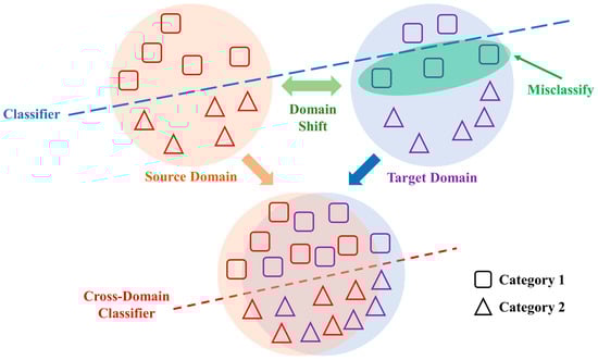
Figure 1. Description of domain shift and domain adaptation.

In order to address the above problems, scholars have developed the domain adaptation (DA) method for diminishing sample distribution discrepancy [11]. Concretely, DA can utilize relevant domain-invariant features extracted from the domain to accomplish a diagnosis task. Meanwhile, many recent studies have shown that DA exhibits encouraging performance on cross-domain works, including semantic correlation transfer [12], handwritten text recognition [13], speaker recognition [14], etc.

Although DA is effective in solving cross-domain problems, most of the existing methods assume that source-domain labels are available for each health state, i.e., all source domain data should be labeled [15,16,17,18]. However, this assumption is almost unpractical in real-world applications. On the one hand, for large rotating machinery, it is impractical to perform massive and detailed full-cycle testing in actual field, because a lot of time must be spent to obtain reliable fault status signals. On the other hand, due to the complexity and uncertainty of mechanical systems, even if vibration signals can be collected in advance, most of the signal labels are unknown. Consequently, source domain labels are insufficient for domain adaptation, resulting in inefficient detection performance. Fortunately, a small number of labeled signals are easily available, and they can be applied to adaptive fault detection.

To overcome the above drawbacks, a semi-supervised adversarial transfer network for cross-domain diagnosis is proposed in this article. Different from the assumption of most existing research, the proposed method does not require a sufficient number of source domain labels for network training. First, a signal-to-image method is adopted to convert vibration signals to images by employing the Gramian Angular Field (GAF). Next, a generative label extension module is designed to generate artificial labels to address the shortage of source domain labels. Then, the artificially labeled data and the labeled data are fed into the dynamic adversarial transfer network for domain adaptation health states detection. In this way, even if most source domain signals lack corresponding labels, the proposed method can still achieve promising performance in dealing with cross-domain tasks. The contributions of this paper are summarized below:

• A novel adversarial domain adaptation networks is proposed to recognize the health conditions of rolling bearings. In addition to adopting a signal processing method to provide more comprehensive characterization for feature extraction, an adversarial domain adaptation approach is also introduced to optimize the cross-domain data distributions, which is beneficial to fault diagnosis under significant changes in the working conditions.
• A semi-supervised learning (SSL)-based label generating module is designed to address the issue of insufficient source domain labels. The generalized features are extracted using consistency regularization and pseudo-labeling. Then, the artificial labels are determined by predicted their probability. Both of them are applied in source domain label generation for intelligent fault detection.

The remainder of this literature begins with a review of related works in Section 2. The proposed intelligent fault detection approach is provided in Section 3. Experimental validation is performed to evaluate the proposed method in Section 4. Section 5 concludes this literature.

2. Related Works

2.1. Research on Intelligent Data-Driven Fault Diagnosis

The related literature about applications of fault diagnosis is summarized in Table 1, which is divided into three categories in terms of detection technologies such as deep learning, maximum mean discrepancy (MMD), and domain adversarial learning. Data-driven health condition detection approaches are reaching remarkable strengths in handling machinery health condition signaling [19,20,21]. In particular, deep learning has attracted increasing attention in related research; thus, the basic fault diagnosis problems that arise from source data and target domain data obeying the same distribution have been well solved [22,23]. Meanwhile, due to increasing demand for generalization ability of monitor and diagnosis models in industry, the transfer learning has been widely used to shrink distribution variance of the feature representations [24]. Currently, most of the domain shift problem has been handled using domain adaptation methods [25], and shallow domain-invariant features are extracted by optimizing the distribution network [26,27]. Han et al. [28] proposed a novel transfer diagnosis approach to sparse target data to minimize distribution discrepancy and address the issue of label space mismatching. A deep convolutional neural-based diagnosis methodology was designed by Azamfar et al. [29] to monitor health conditions and optimize the data distribution of the ball screw. Qian et al. [30] considered the discriminative feature learning in network, and realized fault diagnosis by building a deep discriminative transfer learning network (DDTLN). Huang et al. [31] proposed a new transfer alignment method to solve the problem of the large data differences across domains. However, in the current literature, research on domain adaptation detection with insufficient source domain labels is still limited.

In addition, the distance measurement is also an important issue of transfer learning. Among many distance measures, the MMD is one of the most widely applied distance metrics in transfer learning, which is to find difference between two probability distributions by mapping the data to another space [32,33,34]. By optimizing the MMD metric, the domain distance can be minimized, and the extraction of generalized knowledge can also be promoted. Lu et al. [35] proposed a novel domain adaptation model based on a deep neural network for fault diagnosis, which realized the diagnosis by minimizing MMD and enhancing representative features. Zhang et al. [36] proposed a sparse filtering-based domain adaptation (SFDA) model to obtain high-dimensional features in cross-domain diagnosis tasks, in which l1 norm and l2 norm were implemented on MMD. And a cross-senor domain adaptation approach is proposed by Pandhare et al. [37] to achieve indirect measurement of sensors and diminish the MMD of high-level representations.

In addition to the popular MMD metric, the domain adversarial network developed from the generated adversarial network (GAN) has also become an effective diagnosis method because of its powerful capability to grasp domain generalization features [38,39]. Ganin et al. [40] added an adversarial mechanism to the training of neural network firstly, and called the resulting network a domain adversarial neural network (DANN). Moreover, the domain adversarial network demonstrated excellent performance in fault diagnosis in recent years. Hu et al. [41] presented a hybrid fault diagnosis model based on data augmentation generative adversarial networks (DAGAN) and DANN, wherein they effectively utilized a small amount of sample data to realize fault diagnosis under different working conditions. The novel deep subdomain adaptation graph convolution neural network was proposed by Ghorvei et al. [42], and the adversarial network and structured subdomain adaptation were adopted for reducing the distribution differences. In fields of industrial applications, Guo et al. [43] proposed a reconstruction domain adaptation transfer network, which contributes to identify health conditions and extract domain-invariant features. The recent advances in domain adaptation approaches have been well reviewed [44,45], where the adversarial transfer network has achieved high test accuracy on fault transfer tasks across domains.

Although the domain adaptation technology in the existing fault diagnosis methods have developed rapidly, most methods generally assume that all labels of source domain training data are available during training process. However, it is almost impossible to satisfy this assumption in the real industry. Currently, little research can be found in diagnosis studies of artificial label generation in source domain data. This paper aims at bridging the distribution gap and addressing the cross-domain problem of insufficient source domain labels under diverse operating conditions.

Table 1. Summary of relevant literature on fault diagnosis applications.

Technologies	References	Methodologies
Deep learning	Shen et al. [24]	A transfer approach with the TrAdaBoost algorithm for bearing fault diagnosis.
	Han et al. [28]	A deep transfer diagnosis framework for dealing with limited sparse target data.
	Azamfar et al. [29]	A deep learning-based diagnosis approach for ball screw across domain.
	Qian et al. [30]	The DDTLN model for intelligent cross-machine fault transfer diagnosis.
	Huang et al. [31]	A deep multisource transfer learning model for bearing fault diagnosis.
Maximum mean discrepancy	Xiao et al. [33]	A feature-adaptive motor fault diagnosis method applying MMD as parameter constraint.
	Yang et al. [34]	A diagnosis model based on polynomial kernel induced MMD reused for detection knowledge across machines.
	Lu et al. [35]	A DNN model for domain adaptation in fault detection minimizes the distribution discrepancy between data by maximizing MMD.
	Zhang et al. [36]	A sparse filtering domain adaption approach that incorporates l1-norm and l2-norm for maximizing MMD.
	Pandhare et al. [37]	An indirect sensing fault diagnosis method for domain alignment by minimizing MMD marginal distribution.
Domain adversarial learning	Li et al. [38]	A machinery diagnosis method for partial domain adaptation using conditional data alignment and unsupervised prediction consistency.
	Hu et al. [41]	A hybrid fault diagnosis model based on DAGAN and DANN utilizing a few data to accomplish domain adaptation.
	Ghorvei et al. [42]	A spatial subdomain adaption graph convolution neural network applying adversarial domain adaptation and local MMD to reduce structural discrepancy between domains.
	Guo et al. [43]	A reconstruction domain adaptation transfer network for cross-domain invariant features extraction and equipment health condition detection.

Table 1. Summary of relevant literature on fault diagnosis applications.

Technologies	References	Methodologies
Deep learning	Shen et al. [24]	A transfer approach with the TrAdaBoost algorithm for bearing fault diagnosis.
	Han et al. [28]	A deep transfer diagnosis framework for dealing with limited sparse target data.
	Azamfar et al. [29]	A deep learning-based diagnosis approach for ball screw across domain.
	Qian et al. [30]	The DDTLN model for intelligent cross-machine fault transfer diagnosis.
	Huang et al. [31]	A deep multisource transfer learning model for bearing fault diagnosis.
Maximum mean discrepancy	Xiao et al. [33]	A feature-adaptive motor fault diagnosis method applying MMD as parameter constraint.
	Yang et al. [34]	A diagnosis model based on polynomial kernel induced MMD reused for detection knowledge across machines.
	Lu et al. [35]	A DNN model for domain adaptation in fault detection minimizes the distribution discrepancy between data by maximizing MMD.
	Zhang et al. [36]	A sparse filtering domain adaption approach that incorporates l1-norm and l2-norm for maximizing MMD.
	Pandhare et al. [37]	An indirect sensing fault diagnosis method for domain alignment by minimizing MMD marginal distribution.
Domain adversarial learning	Li et al. [38]	A machinery diagnosis method for partial domain adaptation using conditional data alignment and unsupervised prediction consistency.
	Hu et al. [41]	A hybrid fault diagnosis model based on DAGAN and DANN utilizing a few data to accomplish domain adaptation.
	Ghorvei et al. [42]	A spatial subdomain adaption graph convolution neural network applying adversarial domain adaptation and local MMD to reduce structural discrepancy between domains.
	Guo et al. [43]	A reconstruction domain adaptation transfer network for cross-domain invariant features extraction and equipment health condition detection.

2.2. The ResNet Module

Convolutional neural networks (CNNs) are highly similar to ordinary neural networks, both consisting of neurons that can learn weights and biases. Each neuron receives input and performs the corresponding dot product calculation, then outputs the score of each classification [46]. The difference between the two is that CNN’s use images as an input of, so that specific attributes can be encoded into the network structure and reduce parameters effectively.

There are three prime layers in CNN: the convolutional layer, pooling layer, and fully connected (FC) layer. First, each convolutional layer is made up of several convolutional units, and the backpropagation algorithm optimizes the parameters of each convolutional unit. The convolution operation’s goal is to extract features from the input. Only some low-level features, such as edges or lines, can be extracted using the low-level convolution layer. With the deepening of layers, more complex features can be extracted. Second, since features with larger dimensions are acquired after the convolution layer, in order to obtain features with lower dimensions, the features are divided into several parts and their maximum or average values are acquired in the pooling layer. Finally, the FC layer transforms local features to global features to calculate predicted value for each classification.

With the deepening of network layers, the accuracy of the network is also constantly improved, and ultimately reaches the maximum value (accuracy saturation). Unfortunately, when it reaches a certain depth, the precision of the model drops sharply. This phenomenon, which is contrary to the cognition of scholars, is named degeneration. It was found subsequently that degeneration occurs because the deepening of the network causes gradient explosion and gradient disappearance.

To address degeneration, He et al. [47] presented the ResNet model. The idea of ResNet was mainly derived from VLAD [48] (the source of ideas for residuals) and the highway network [49] (the source of ideas for skipping connections). First, for a stacked layer structure (several layers are stacked on top of each other), let the input be $x$. Then, the learned feature is denoted as $\mathcal{H}\left(x\right)$ and the learned residuals from the network are $\mathcal{F}\left(x\right)=\mathcal{H}\left(x\right)-x$. Therefore, it can be inferred that the primitive extracted feature is $\mathcal{H}\left(x\right)=\mathcal{F}\left(x\right)+x$. This is due to the fact that learning residuals is easier than directly learning original features. Although the stacking layer only executes identity mapping, the network performance does not deteriorate when the residual is zero. The residuals will not actually be zero, so that the stacked layers are allowed to learn new features and provide better optimization performance for the model. The structure of the residual learning unit is shown in Figure 2. The building block is denoted as

$$y=\mathcal{F}\left(x,\left\{W_i\right\}\right)+x$$

(1)

where $y$ is stands for the output vectors of the regarded layer. The function $\mathcal{F}\left(x,\left\{W_i\right\}\right)$ is the residual mapping studied by the building block. And the dimensions of $x$ and $\mathcal{F}$ must be equal. When the dimensions of the input or output channels do not match, the linear projection $W_s$ is conducted using shortcut connection to match the dimensions:

$$y=\mathcal{F}\left(x,\left\{W_i\right\}\right)+W_{s}x$$

(2)

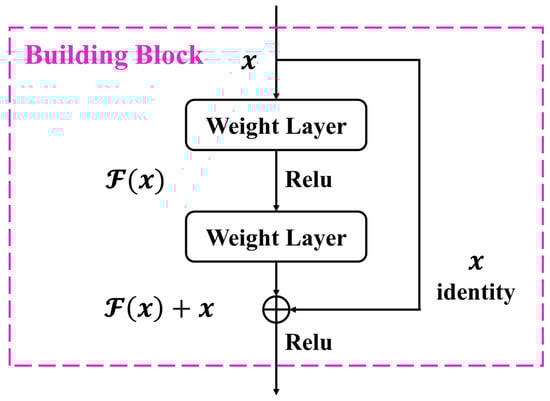
Figure 2. A building block in residual learning.

3. Proposed Method

3.1. Problem Formulation

Generally, this study was conducted under the following assumptions:

• Due to the diversity in operating conditions, although the source domain and the target domain are interrelated, they follow the distinct distributions.
• The purpose of intelligent fault diagnosis in various domains is consistent.
• The source-domain data (whether labeled or unlabeled) and all unlabeled data from the target domain can be employed to train networks.
• During training, not only are signals from the target domain unlabeled, but most signals from the source domain are also unlabeled.

The above assumptions simulate the actual industrial situation where signal labels are insufficient, i.e., a large amount of vibration signals can be collected, but only a small part of them have health condition labels. Existing methods cannot obtain satisfactory diagnosis results.

Let $\mathit{X}$ denote the input signal space and $\mathit{Y}=\left\{1,2,\dots ,N_c\right\}$ represent the set of $N_c$ health conditions, for any sample $\left(x_i,y_i\right)$ with $x_i\in \mathit{X},y_i\in \mathit{Y}$. A partial unlabeled source domain ${\mathcal{D}}_s$ of $n_s$ samples and an unlabeled target domain ${\mathcal{D}}_t$ of $n_t$ samples are available. The ${\mathcal{D}}_s$ and the ${\mathcal{D}}_t$ can be formulated as

$${\mathcal{D}}_s={\left\{\left(x_i^s,y_i^s=C_h\right)\right\}}_{i=1}^{n_{su}}\cup {\left\{\left(x_i^s,y_i^s\right)\right\}}_{i=n_{su}+1}^{n_{sl}}$$

(3)

$${\mathcal{D}}_t={\left\{\left(x_j^t,y_j^t=0\right)\right\}}_{j=1}^{n_t}$$

(4)

where $\left(x_i^s,y_i^s\right)$ and $\left(x_i^t,y_i^t\right)$ denote the samples of $\left(x_i,y_i\right)$ in ${\mathcal{D}}_s$ and ${\mathcal{D}}_t$, respectively; $C_h$ denotes the labeled machine health conditions; $n_{su}$ and $n_{sl}$ mean the number of unlabeled and labeled source domain data, respectively; and $n_s=n_{su}+n_{sl}$. Similarly, $n_t$ denotes the amount of target domain data. ${\mathcal{D}}_s$ and ${\mathcal{D}}_t$ are sampled from joint distributions $P_s\left(\mathit{X},\mathit{Y}\right)$ and $P_t\left(\mathit{X},\mathit{Y}\right)$, and $P_s\ne P_t$. Particularly, since the label spaces of the source and target domains are identical in this paper, ${\mathcal{D}}_s$ and ${\mathcal{D}}_t$ are considered as being sampled from various marginal distributions—$P_s\left(\mathit{X}\right)$ and $P_t\left(\mathit{X}\right)$.

The purpose of this paper is to generate a source domain pseudo-label data set $D_s^{Pseudo}={\left\{\left(x_i^s,y_i^s\ne C_h\right)\right\}}_{i=1}^{n_{su}}\cup {\left\{\left(x_i^s,y_i^s\right)\right\}}_{i=n_{su}+1}^{n_{sl}}$ of $n_{su}$ signals in operating conditions based on ${\mathcal{D}}_s$. The $D_s^{Pseudo}$ is defined with the following formula:

$$D_s^{Pseudo}={\left\{\left(x_i^s,y_i^s\ne C_h\right)\right\}}_{i=1}^{n_{su}}\cup {\left\{\left(x_i^s,y_i^s\right)\right\}}_{i=n_{su}+1}^{n_{sl}}$$

(5)

Afterwards, feature extractors and domain discriminators are constructed for minimizing the feature extractor loss and maximizing the discriminator loss so as to retrieve generalization features and reduce the network loss.

3.2. The Hybrid Networks

Aiming at the dilemma of fault detection under diverse operating conditions in the absence of sufficient labeled data, this study proposes a semi-supervised adversarial transfer network for cross-domain diagnosis. Firstly, a signal-to-image conversion method for 1D signal processing is presented. Secondly, a generative label extension network based on SSL is designed to predict and generate artificial labels. Finally, a dynamic adversarial transfer network is proposed for domain adaptation feature knowledge extraction and fault detection classification. An overview of the proposed condition monitoring approach is presented in Figure 3.

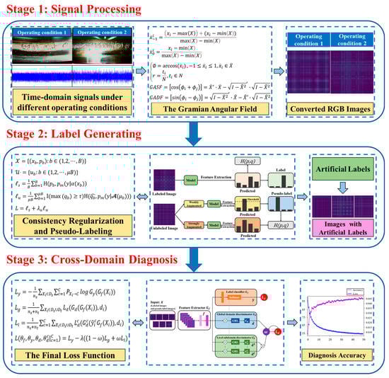
Figure 3. The flow diagram of the proposed approach.

3.2.1. Stage 1: Signal Processing

As we have seen, deep learning has advanced considerably in intelligent condition diagnosis, but it fails to preserve temporal dependency entirely when processing time domain vibration signals, which leads to a loss of data signals. Furthermore, existing networks such as recurrent neural network are difficult to train; hence, it is hard to construct accurate monitoring models. However, by converting time domain vibration signals into 2D image dataset through GAF, not only can enrich signal characteristics by filling vibration signals with pixels, but also establish bijective mapping between 1D vibration signals and 2D space to ensure the integrity of information.

Since the inner product operation cannot retain both observed values during conversion process, both of them can only be converted into one value. To avoid this loss of information, Gram-like matrix is generated by calculating $x\oplus y=\cos \left({\theta }_1+{\theta }_2\right)$, so that original values of scaled time series form diagonal lines, and 1D vibration signals are approximately reconstructed with advanced features extracted by deep learning, so as to maintain an absolute temporal relationship [50].

Therefore, it is crucial to convert 1D time series signals into 2D images efficiently [51]. And the GAF is offered to convert 1D time series into RGB images in this study. Assume a time series $X=\left\{x_1,x_2,\cdots ,x_n\right\}$ of n real-valued observations, then rescale the time series $X$ to keep all values are in the interval (–1, 1) or (0, 1) by:

$${\tilde{x}}_{-1}^i=\frac{\left(x_i-\max \left(X\right)\right)+\left(x_i-\min \left(X\right)\right)}{\max \left(X\right)-\min \left(X\right)}$$

(6)

$${\tilde{x}}_0^i=\frac{x_i-\min \left(X\right)}{\max \left(X\right)-\min \left(X\right)}$$

(7)

where ${\tilde{x}}_{-1}^i$ and ${\tilde{x}}_0^i$ represent the values of $x_n$ falling within the interval (–1, 1) or (0, 1).

Therefore, the rescaled time series $\tilde{X}$ in polar coordinates can be obtained by encoding the value as the angular cosine and the time stamp as the radius, and the corresponding formula is as follows:

$$\left\{\begin{array}{l}\varnothing =\arccos \left({\tilde{x}}_i\right),-1\le {\tilde{x}}_i\le 1,{\tilde{x}}_i\in \tilde{X}\\ r=\frac{t_i}{N},t_i\in \mathbb{N}\end{array}\right.$$

(8)

where $t_i$ is the time stamp and $N$ denotes a constant factor to regularize the span of the polar coordinate system.

The encoding map of Equation (8) has several advantages. First, since it is bijective, the original time series can be reconstructed by using $\theta$ and $r$. Second, the time dependence in the original time series is preserved through the coordinates of $r$.

Additionally, it can be seen from Equation (8) that (–1, 1) represents the cosine function in (0, π) and the cosine value decreases monotonically within this range. Likewise, (0, 1) denote the cosine function in $\left[0,\frac{\pi }{2}\right]$. By calculating the cosine of the angle sum between various points, the GAF can generate two different images, i.e., the Gramian angular summation field (GASF) and the Gramian angular difference field (GADF). The two are, respectively, represented by the following formulas:

$$GASF=\left[\cos \left({\varphi }_i+{\varphi }_j\right)\right]={\tilde{X}}^{\prime }·\tilde{X}-{\sqrt{I-{\tilde{X}}^2}}^{\prime }·\sqrt{I-{\tilde{X}}^2}$$

(9)

$$GADF=\left[\sin \left({\varphi }_i-{\varphi }_j\right)\right]={\sqrt{I-{\tilde{X}}^2}}^{\prime }·\tilde{X}-{\tilde{X}}^{\prime }·\sqrt{I-{\tilde{X}}^2}$$

(10)

where $I$ denotes the unit row vector (1, 1, ···, 1).

In short, we only need to rescale the time series X into the polar coordinate system using Equation (8), then utilize the corresponding equation to calculate; finally, we can obtain the image from the GASF and GADF. The diagram of the above transformation is presented in Figure 4. In this study, we use GASF to convert 1D vibration signals into images.

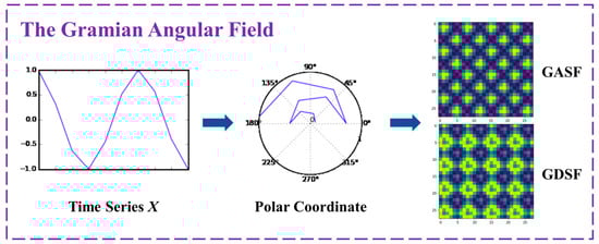
Figure 4. Diagram of the GAF conversion process.

3.2.2. Stage 2: Label Generation

In traditional fault diagnosis method, the accuracy of diagnosis model is determined by the quantity of data labels. Cross-domain diagnostic tasks cannot be performed if there are sufficient signals but not enough labels [52]. Specifically, SSL can provide an effective approach to reducing the dependence on labeled data by using unlabeled data [53]. Therefore, this paper introduces an SSL-based generative label extension network, which utilizes unlabeled images to predict and generate artificial labels. The generated labels can be used for subsequent transfer learning to improve the accuracy of diagnosis models.

First, we define $\mathcal{X}=\left\{\left(x_b,{\mathit{p}}_b\right):b\in \left(1,2,\cdots ,B\right)\right\}$ as a batch of B-labeled samples for an L-class classification problem, where $x_b$ are the training examples and ${\mathit{p}}_b$ denotes one-hot labels. Then, let $\mathcal{U}=\left\{u_b:b\in \left(1,2,\cdots ,\mu B\right)\right\}$ be a batch of $\mu B$ unlabeled examples where $\mu$ is a hyperparameter used to dictate the relevant sizes of $\mathcal{X}$ and $\mathcal{U}$. ${\mathit{p}}_m\left(y|x\right)$ is the prediction category distribution generated by the input $\mathcal{X}$. Additionally, we define $H\left(\mathit{p},\mathit{q}\right)$ as the cross-entropy between two probability distributions p and q. Finally, two types of augmentations are leveraged in the proposed method: strong and weak, denoted by $\mathcal{A}\left(\cdot \right)$ and $\alpha \left(\cdot \right)$, respectively. In this work, weak augmentation makes use of standard flip-and-shift strategy, while strong augmentation first uses RandAugment [54] or CTAugment [55], then uses CutOut [56] to enhance images; severely distorted input images are output in the end.

The training process consists of two parts as depicted in Figure 5: supervised training and unsupervised training. Labeled data perform supervised training, and conventional classification tasks are carried out to reduce the supervised loss. For unlabeled data, use their weakly-augmented versions to train the model to output predictions. When the probability for a class is higher than the threshold, the prediction of that class is considered a pseudo-label. Next, this pseudo-label is used to supervise the output of a strongly-augmented version of the same image.

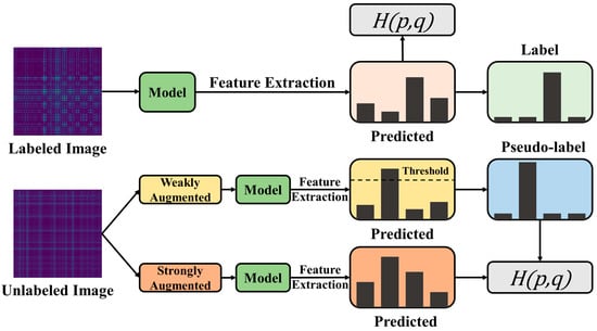
Figure 5. The flowchart of label generative module.

The detailed training process is as follows:

Step 1.

Input:

Prepare the labeled batch $\mathcal{X}=\left\{\left(x_b,{\mathit{p}}_b\right):b\in \left(1,2,\cdots ,B\right)\right\}$, the unlabeled batch $\mathcal{U}=\left\{u_b:b\in \left(1,2,\cdots ,\mu B\right)\right\}$, and unlabeled data ratio μ.

Step 2.

Supervised training:

Use the conventional cross-entropy loss $H\left(\mathit{p},\mathit{q}\right)$ for classification task of labeled data, and the supervised loss ${\mathcal{𝓁}}_s$ with labeled data being defined as

$${\mathcal{𝓁}}_s=\frac{1}{B}{\displaystyle \sum }_{b=1}^B\mathsf{H}({\mathit{p}}_b,{\mathit{p}}_m\left(y|\alpha \left(x_b\right)\right))$$

(11)

where $\alpha$ denotes a random function.

Step 3.

Pseudo-labeling:

Apply weak and strong augmentation to unlabeled data to, respectively, obtain augmented data. Then feed them into the model to acquire predictions and select the weakly augmented prediction to generate pseudo-label using argmax.

Step 4.

Consistency regularization:

Compute the cross-entropy loss $H\left(\mathit{p},\mathit{q}\right)$ between strongly augmented predicted value and weakly augmented pseudo-label value; the unsupervised loss ${\mathcal{𝓁}}_u$ of unlabeled data is defined as

$${\mathcal{𝓁}}_u=\frac{1}{\mu B}{\displaystyle \sum }_{b=1}^{\mu B}\mathbb{Z}\left(\max \left({\mathit{q}}_b\right)\ge \tau \right)\mathsf{H}\left(\widehat{{\mathit{q}}_b},{\mathit{p}}_m\left(y|\mathcal{A}\left(u_b\right)\right)\right)$$

(12)

where ${\mathit{q}}_b={\mathit{p}}_m\left(y|\alpha (u_b)\right)$, $\widehat{{\mathit{q}}_b}=\arg \max ({\mathit{q}}_b)$ denotes pseudo-label, τ is a scalar hyperparameter denoting the threshold for pseudo-label, and $\mathbb{Z}\left(\cdot \right)$ represents the indicator function.

Step 5.

Objective loss function:

The training objective is a cross-entropy loss, which can be formulated as:

$$L=l_s+{\lambda }_u{l}_u$$

(13)

where ${\lambda }_u$ denotes the relative weight of unlabeled data loss.

Step 6.

Label generation:

Feed unlabeled data are fed into the model to generate artificial labels for subsequent diagnosis task.

3.2.3. Stage 3: Cross-Domain Diagnosis

Feature extraction is crucial to fault diagnosis. Conventional feature extraction methods are not suitable for cross-domain diagnosis, while adversarial transfer networks can effectively extract domain-invariant features to solve cross-domain problems. Therefore, the adversarial transfer network is combined with the label generation module mentioned in Stage 2 to address the degradation of diagnosis performance due to distribution discrepancy.

Figure 6 shows the architecture of the presented networks. Form the figure, the network is composed of a feature extractor $G_f$, a label classifier $G_y$ applied to identify source-domain labels, a global domain discriminator $G_d$ applied to align marginal distributions of source and target domains, and C local subdomain discriminators $G_d^c(c\in \left\{1,2,\cdots ,C\right\})$ applied to align conditional distributions of source and target domains. In detail, labeled source domain data, target domain data, and pseudo-labeled data in Stage 2 are mixed as the input x of the network; then, the high-level features f are extracted by the feature extractor $G_f$. Then, feature f is fed into $G_f$ and the domain discriminators (including discriminator $G_d$ and $G_d^c$) for adversarial training. Finally, optimal domain-invariant feature extraction is achieved by minimizing the loss $L_y$ and maximizing $L_g$ and $L_l$, where $L_y$ is the loss of $G_f$, $L_g$ is the loss of $G_d$ and $L_l$ is the loss of $G_d^c$. We calculate the losses of $L_y$, $L_g$ and $L_l$ as:

$$L_y=-\frac{1}{n_s}{\displaystyle \sum }_{X_i\in D_s}{\displaystyle \sum }_{c=1}^C{P}_{X_i\to C}\log G_y\left(G_f\left(X_i\right)\right)$$

(14)

$$L_g=\frac{1}{n_s+n_t}{\displaystyle \sum }_{X_i\in D_s\cup D_t}{L}_d\left(G_d\left(G_f\left(X_i\right)\right),d_i\right)$$

(15)

$$L_l=\frac{1}{n_s+n_t}{\displaystyle \sum }_{c=1}^C{\displaystyle \sum }_{X_i\in D_s\cup D_t}{L}_d^c\left(G_d^c\left({\widehat{y}}_i^c{G}_f\left(X_i\right)\right),d_i\right)$$

(16)

where $P_{X_i\to C}$ represents the probability that $X_i$ belongs to class c, and ${\widehat{y}}_i^c$ denotes the predicted probability distribution of the input sample $X_i$ belonging to class C. Moreover, the dynamic adversarial factor ω can dynamically and robustly evaluate the $G_d$ and $G_d^c$ weights according to the difference of data distribution in different diagnostic tasks. The ω is defined as:

$$\widehat{\omega }=\frac{d_{\mathcal{A},g}\left(D_s,D_t\right)}{d_{\mathcal{A},g}\left(D_s,D_t\right)+\frac{1}{C}{{\displaystyle \sum }}_{c=1}^C{d}_{\mathcal{A},l}\left(D_s^c,D_t^c\right)}$$

(17)

where $d_{\mathcal{A},g}\left(D_s,D_t\right)$ and $d_{\mathcal{A},l}\left(D_s^c,D_t^c\right)$ represent the $\mathcal{A}$-distance of global domain discriminator $G_d$ and local domain discriminator $G_d^c$, respectively.

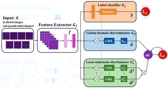
Figure 6. The architecture of the dynamic transfer networks. $\widehat{y}$ denotes predicted label, $L_y$ and $L_d$ represent classification loss and domain loss. $\widehat{d}$ and ${\widehat{d}}^C$ present predicted domain label. GRL means the gradient reversal layer.

By integrating all components, the final objective function of transfer network can be expressed as:

$$L\left({\theta }_f,{\theta }_y,{\theta }_d,{\theta }_d^c{|}_{c=1}^C\right)=L_y-\lambda \left(\left(1-\omega \right)L_g+\omega L_l\right)$$

(18)

In summary, the network maps feature of source and target domain to the same space by confusing the domain labels. By adaptively measuring the distribution difference between the two domains, the target-domain data is labeled using domain-invariant features, which are indistinguishable between source and target domains. In addition, network domain adaptation and feature extraction are performed simultaneously, and label classification is supervised by source domain labels, target domain labels, and domain labels at the same time.

3.3. System and Steps of Diagnosis Process

In general, the raw vibration signal is converted into RGB images using the GAF in Stage 1 firstly, including labeled images and unlabeled images. Secondly, unlabeled images are fed into the network in Stage 2, which combines supervised and unsupervised learning to generate artificial labels. Thirdly, the adversarial transfer network in Stage 3 adaptively reduces distribution discrepancy to extract the generalization features, so as to deliver accurate fault classification results. Using the proposed hybrid networks, the networks realize feature transfer and complete intelligent fault identification of the signal.

Step 1.

Collect one-dimensional bearing vibration signal under diverse operating conditions.

Step 2.

Convert the raw signals collected in Step 1 into two-dimensional images using the GAF.

Step 3.

Divide the two-dimensional images into labeled datasets, unlabeled datasets, and validation datasets according to required proportion, and input them into label generative extension network for training.

Step 4.

Feed the unlabeled data into the label generative extension model to obtain the model prediction for label classification.

Step 5.

Divide the dataset mixed with real and artificial labels into training set and validation set and input the training set into the dynamic adversarial transfer network for cross-domain diagnosis.

Step 6.

Calculate the accuracy of the validation set and output the health state detection results of the model.

4. Case Studies

To verify the capability of the intelligent fault detection networks proposed in this article, two practical case studies were carried out. In case study 1, a comparative experiment of diagnosis performance under diverse working conditions was conducted, and case study 2 compared the diagnosis performance of the proposed method with conventional methods under various label proportions.

4.1. Dataset Descriptions

In this case, the proposed approach is performed on the public datasets acquired from the Bearing Data Center of Case Western Reserve University [57]. Extensive studies have been conducted on this rolling bearing fault diagnosis dataset. The vibration data used in this work were collected from the sensor placed on the drive end of the motor, which ran at a constant speed with four rotating speeds, i.e., 1730, 1750, 1772, 1797 r/min, and on four health conditions, i.e., normal (NO), ball fault (BF), inner race fault (IF), outer race fault (OF). The three different types of artificial faults were created with diameters of 7, 14, 21 mils. In addition, the CWRU experimental platform is shown in Figure 7.

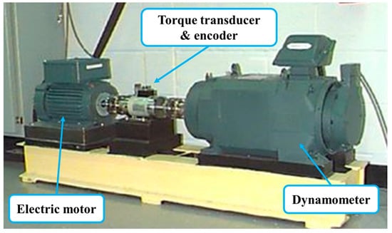
Figure 7. The CWRU bearing test rig.

Ten operation patterns (containing one NO and nine faulty conditions) in four rotating speed domains are included in the CWRU datasets. It is worth noting that the CWRU dataset is widely considered as a publicly available dataset for fault detection of rolling bearings due to its better data quality and less noise interference. In this study, seven operation conditions were selected to examine the proposed method according to the experimental requirements.

In the CWRU dataset, the vibration signal was acquired from the sensor at an operating frequency of 1.2 kHz for about 10 s, and each dataset had about 120,000 data points. Taking into account the above factors, performing data truncation on the original signal is critical. Therefore, in this article, a sliding window truncation method is proposed to generate a dataset for seven operation patterns. As depicted in Figure 8, a truncation window slides along the vibration signal at a shift length of 64 data points, and the window size is 512 data points. Therefore, the signal is converted into a dataset consisting of 512 × 512 RGB images under the action of the sliding window. The converted results are presented in Figure 9. For example, BF-07 indicates a ball fault with a fault diameter of 7 mils, IF-14 indicates an inner race fault with a fault diameter of 14 mils, and the rest follow the same pattern.

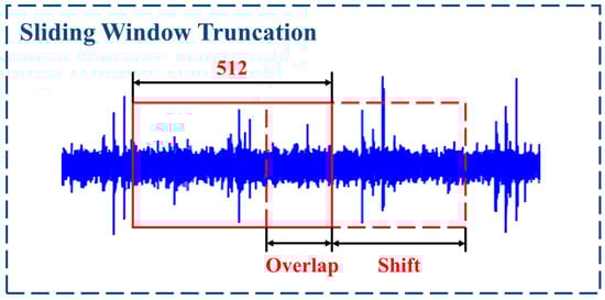
Figure 8. The sliding window truncation method.

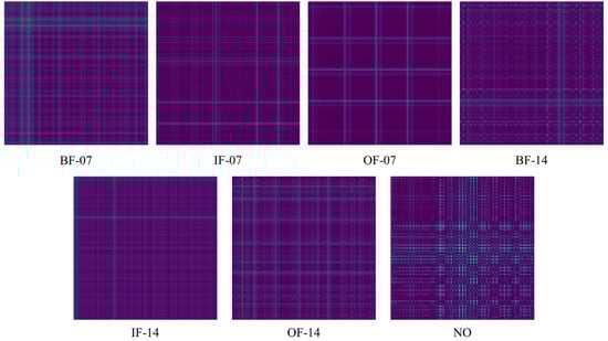
Figure 9. Converted images in this work.

4.2. Case Study 1: Variable Operating Conditions Transfer Experiment

Utilizing the sliding window truncation method, the raw vibration signal is processed into datasets under four different load scenarios (0, 1, 2, 3 HP) using the GAF. The dataset of each scenario contains seven types of faults, and each type of fault has 600 images. Thus, there are a total of 4200 images for operating conditions, and each dataset is randomly divided into the training dataset and testing dataset according to a ratio of 8:2. Detailed data descriptions of the dataset are presented in Table 2.

Table 2. The CWRU dataset details for each operating condition.

Class Label	1	2	3	4	5	6	7	Train/Test
Fault location	NO	BF	BF	IF	IF	OF	OF	3360/840
Fault size (mil)	0	7	14	7	14	7	14

In this case, the variable working conditions transfer experiment is mainly evaluated by the proposed method in these 12 tasks, i.e., ${\mathrm{T}}_{01}$, ${\mathrm{T}}_{02}$, ${\mathrm{T}}_{03}$, ${\mathrm{T}}_{10}$, ${\mathrm{T}}_{12}$, ${\mathrm{T}}_{13}$, ${\mathrm{T}}_{20}$, ${\mathrm{T}}_{21}$, ${\mathrm{T}}_{23}$, ${\mathrm{T}}_{30}$, ${\mathrm{T}}_{31}$, ${\mathrm{T}}_{32}$. For example, ${\mathrm{T}}_{01}$ represents a variable operating condition transfer task with 0 HP load as the source domain and 1 HP load as the target domain. The rest of symbols T follow the same pattern as well. Part of the transfer details are shown in Table 3, where labeled proportion represents the proportion of labeled images in the training dataset.

Table 3. Partial details of fault diagnosis tasks in this case.

Task	Source	Target	Labeled Proportion
${\mathrm{T}}_{01}$: 0$\to$1	1797 rpm	1772 rpm	$\frac{1}{2}$
${\mathrm{T}}_{12}$: 1$\to$2	1772 rpm	1750 rpm	$\frac{1}{2}$
${\mathrm{T}}_{23}$: 2$\to$3	1750 rpm	1730 rpm	$\frac{1}{2}$

In this experiment, there are seven types of images, totaling 4200 images fed into the hybrid network, of which 3360 images were divided into training dataset and 840 images were divided into testing dataset. Then, half of the training data are randomly selected as labeled data and the remaining training data are treated as unlabeled data. The labeled data and unlabeled data are sent to the label generation model for training, and the artificial label prediction results of unlabeled data are output. Next, the labeled data and the artificially labeled data are imported together into the dynamic adversarial transfer network for training until the network converges. Finally, an accurate cross-domain fault diagnosis model is obtained. To illustrate effectiveness, the results of different transfer tasks are compared. In addition, average identification accuracy is selected as the model measurement standard; the accuracy is the average value of 10 rounds of experiments. Table 4 shows the comparison results.

Table 4. Comparison results.

Task Name	Motor Loads	Number of Labeled Data	Average Accuracy
${\mathrm{T}}_{01}$	0$\to$1	1680	99.88%
${\mathrm{T}}_{02}$	0$\to$2	1680	99.26%
${\mathrm{T}}_{03}$	0$\to$3	1680	99.38%
${\mathrm{T}}_{10}$	1$\to$0	1680	98.25%
${\mathrm{T}}_{12}$	1$\to$2	1680	99.28%
${\mathrm{T}}_{13}$	1$\to$3	1680	98.71%
${\mathrm{T}}_{20}$	2$\to$0	1680	98.62%
${\mathrm{T}}_{21}$	2$\to$1	1680	99.71%
${\mathrm{T}}_{23}$	2$\to$3	1680	99.64%
${\mathrm{T}}_{30}$	3$\to$0	1680	98.15%
${\mathrm{T}}_{31}$	3$\to$1	1680	99.42%
${\mathrm{T}}_{32}$	3$\to$2	1680	99.72%

It can be seen from Table 3 that the proposed method can maintain an average accuracy of more than 99.17% in fault detection under diverse operating conditions, which indicates that the designed approach has powerful ability to solve the seven classifications problem with high efficiency. To sum up, this method can still maintain high accuracy of cross-domain label recognition under various working conditions, as well as in the absence of some source-domain labels, thus demonstrating the effectiveness of the fault transfer diagnosis network proposed in this article.

Taking task ${\mathrm{T}}_{31}$ as an example, the accuracy and loss curves of the model are shown in Figure 10. With the increase in training epochs, the accuracy of the fault label classifier was continuously improved, approaching 99% in 50 epochs and tended to be stable. Meanwhile, the testing loss gradually declined until it approached 0.0087 within about 40 epochs, then kept stable. From the result, it can be inferred that after sufficient training epochs, the proposed network can effectively extract domain-invariant features of vibration signals and accurately perform cross-domain detection, which indicates that the designed diagnosis network is reasonable.

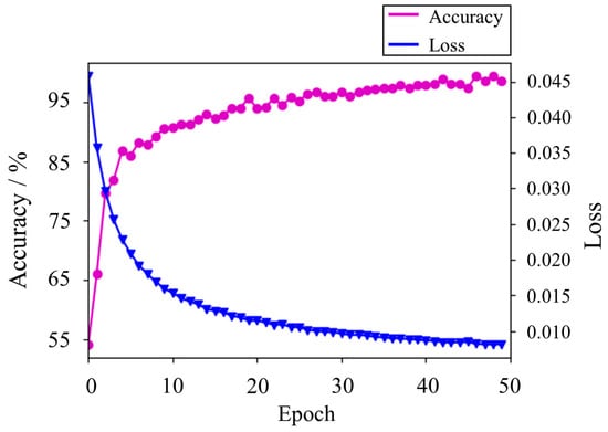
Figure 10. Training accuracy and loss curves.

Next, the influence of the evaluation metrics was investigated. In addition to accuracy, precision, recall, and F1 score were selected to evaluate the validity of the fault detections. Three representative tasks, ${\mathrm{T}}_{01}$, ${\mathrm{T}}_{12}$, and ${\mathrm{T}}_{23}$, were used as examples for analysis, and the results are shown in Figure 11. It can be observed that the overall evaluation metrics of the three tasks are above 99.2%, and ${\mathrm{T}}_{01}$, ${\mathrm{T}}_{23}$, and ${\mathrm{T}}_{12}$ decrease sequentially. Specifically, precision, recall, and F1 score of each task were relatively stable and close to their corresponding precision. The satisfactory transfer performance between domains was achieved using the proposed networks, which demonstrates that the proposed networks are suitable for domain adaptation with high robustness.

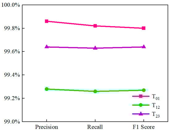
Figure 11. The precision, recall, and F1 score for ${\mathrm{T}}_{01}$, ${\mathrm{T}}_{12}$ and ${\mathrm{T}}_{23}$.

Furthermore, Figure 12 presents the fault diagnosis result of ${\mathrm{T}}_{21}$ after ten repeated calculations by using the confusion matrix. The vertical axis of the confusion matrix denotes the true label, and the horizontal axis is the predicted label. From the figure, it can be seen that the average detection accuracy of the seven health states is 99.7%; the diagnosis performance is satisfactory. Specifically, IF-07, OF-07, BF-14, and NO all have 100% detection accuracy, which implies that they have not assigned the label to others, with BF-14 having received the wrong category from IF-14. BF-07 and OF-14 can accept the error misclassification of each other. BF-07 has the lowest accuracy rate of 98.8%, and more BF-07 elements are assigned to OF-14. The results indicated that even though half of training data lack health condition labels, the proposed approach can still achieve the precise diagnosis of seven health conditions in the target domain. Thus, the effectiveness of the proposed approach for domain adaptation detection is verified in the presence of insufficient labels.

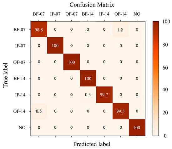
Figure 12. Confusion matrix of fault detection results.

Furthermore, Figure 13 shows the ROC curve of the fault diagnosis result of task ${\mathrm{T}}_{23}$. As can be seen from the figure, all the fault classification curves coincide, for except some deviation in the OF-14 curve, where the IF-07 and OF-07 curves overlap with the NO curve. This means that seven kinds of bearing fault classification can be perfectly diagnosed by using proposed networks, which also proves the validity of the proposed networks.

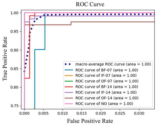
Figure 13. The ROC curve of fault diagnosis result.

4.3. Case Study 2: Insufficient Source Domain Label Transfer Experiment

To highlight the effectiveness of the proposed networks in fault detection on small samples of labeled data, this experiment further expands the gap between the number of labeled and unlabeled data in the source domain. For the vibration signal data collected at the sampling frequency of 12 kHz, 1/2, 1/4, 1/8, and 1/16 of the source domain images are selected as labeled data, and the rest are unlabeled data. Moreover, the diagnostic tasks ${\mathrm{T}}_{01}$, ${\mathrm{T}}_{12}$, ${\mathrm{T}}_{23}$, ${\mathrm{T}}_{21}$, and ${\mathrm{T}}_{31}$ are performed for experimental evaluations.

In this case study, experiments were conducted to compare the proposed networks with three other commonly used transfer learning models, namely deep adaptation network (DAN), Deep CORAL, and DANN. The structure of the CNN feature extractor used for comparison is the same as that of the proposed networks, and each group of trials was performed 10 times and averaged.

The diagnosis accuracies of the proposed method were compared with other popular transfer methods, the comparison results are shown in Table 5. From the comparison results, it can be seen that the network proposed in this experiment can still identify fault labels with an average accuracy of 98.32%, even though the number of labeled samples is only one in sixteen. Moreover, compared to the other transfer models, the accuracy fluctuation of the proposed model tends to be stable when the labeled proportion is changed. This illustrates the excellent robustness of the proposed method in extreme cases. On the other hand, the proposed networks produce higher detection accuracy than other diagnosis models, and are always higher than DANN. This is because the proposed model dynamically adjusts the proportion of marginal distribution and conditional distribution when extracting domain-invariant features, while DANN only considers the adaptation of marginal distribution.

Table 5. Average testing accuracies in the fault detection of case study 2.

Method	DAN				Deep CORAL				DANN				Proposed
Proportion	1/2	1/4	1/8	1/16	1/2	1/4	1/8	1/16	1/2	1/4	1/8	1/16	1/2	1/4	1/8	1/16
0$\to$1	98.92	97.58	94.68	91.12	98.77	97.63	93.95	92.87	99.54	98.87	97.16	97.02	99.80	99.12	98.06	97.23
1$\to$2	97.20	96.47	94.89	94.78	97.88	96.83	95.85	93.40	98.72	97.96	96.11	95.86	99.28	99.07	97.73	97.19
2$\to$3	98.46	95.89	93.94	93.17	97.70	97.14	94.23	93.00	99.21	98.59	96.72	94.33	99.64	99.31	97.66	96.54
2$\to$1	95.90	94.36	93.08	92.84	95.30	94.36	92.17	92.05	98.58	97.78	95.62	94.22	99.70	98.69	96.44	96.10
3$\to$2	98.12	97.37	96.63	95.90	98.31	96.87	96.05	94.71	98.95	98.22	97.62	96.41	99.72	98.98	98.79	97.38
Average	97.72	96.33	94.64	93.56	97.59	96.57	94.45	93.21	99.00	98.28	96.65	95.57	99.63	99.03	97.74	96.89

Figure 14 manifests that with the decrease in labeled data in source domain, the proposed model still maintains high accuracy, while other transfer learning methods exhibit the overfitting phenomenon. It also indicates that when the labeled data are insufficient, the proposed method can effectively alleviate the overfitting phenomenon, and provide high accuracy results. Additionally, transfer adversarial networks are proven to maximize the utilization of limited labeled data.

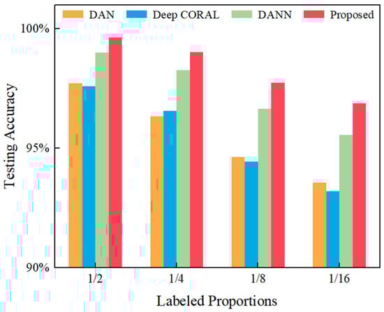
Figure 14. Comparison of contrast test accuracy.

To visually present the training results of different transfer models, taking the 1/16 experiment as an example, t-SNE dimensionality reduction processing was performed on the last hidden layer of DAN, Deep CORAL, DANN, and the proposed networks, respectively. The features were plotted into the 2D space, and the outcome of the visualization is shown as Figure 15.

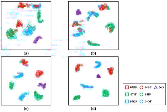
Figure 15. Visualizations of the learned feature representations in the fully connected layer in the feature extractor: (a) DAN; (b) Deep CORAL; (c) DANN; (d) Proposed.

Figure 15 depicts that all four methods can separate the fault classifications from the original distribution, but the DAN network and the Deep CORAL network cannot completely overcome the difference in feature marginal distribution, and it is prone to the negative transfer phenomenon when there are few available labeled data. On the other hand, the approach proposed in this study projects all types of labels perfectly to the same area, demonstrating significant clustering and separability. This is sufficient to show that the proposed networks can perform cross-domain operation states detection reliably in the case of less available label data.

5. Conclusions

Aiming at the domain shift problem in the case of insufficient source domain labels, a method of applying semi-supervised adversarial transfer networks for cross-domain fault detection was proposed in this literature. Initially, vibration signals were converted into images using the signal-to-image method. Furthermore, a semi-supervised generation module was designed to generate artificial labels for unlabeled images, so as to solve the dilemma of insufficient source domain labels. Eventually, the adversarial transfer networks were introduced to extract domain-invariant features in different domains and achieve fault detections. Two case studies were conducted on the public rolling bearing dataset to validate the performance of the proposed approach. The analysis results clarify that the proposed networks are able to diminish the distribution discrepancy and extract generalized features for domain adaptation detection. Meanwhile, the generalization and robustness of the proposed networks were demonstrated by carrying out a cross-domain transfer experiment and insufficient source-domain label experiment. Therefore, the finding of this research has great potential in practical applications, since comprehensive experimental data on health status labels are generally hard to acquire in the real industry.

Although the proposed approach is effective for processing common cross-domain diagnosis problems, when the training data in each health state are unbalanced, diagnostic accuracy is dramatically degraded. To address this issue, future research will be considered to perform accurate and efficient fault detection in the presence of an unbalanced health state dataset.

References

- Glowacz, A.; Glowacz, W.; Kozik, J.; Piech, K.; Gutten, M.; Caesarendra, W.; Liu, H.; Brumercik, F.; Irfan, M.; Faizal Khan, Z. Detection of Deterioration of Three-phase Induction Motor using Vibration Signals. Meas. Sci. Rev. 2019, 19, 241–249. [Google Scholar] [CrossRef]
- Caesarendra, W.; Tjahjowidodo, T. A Review of Feature Extraction Methods in Vibration-Based Condition Monitoring and Its Application for Degradation Trend Estimation of Low-Speed Slew Bearing. Machines 2017, 5, 21. [Google Scholar] [CrossRef]
- Wang, Z.; Wang, J.; Cai, W.; Zhou, J.; Du, W.; Wang, J.; He, G.; He, H. Application of an Improved Ensemble Local Mean Decomposition Method for Gearbox Composite Fault Diagnosis. Complexity 2019, 2019, 1–17. [Google Scholar] [CrossRef]
- Bazan, G.H.; Goedtel, A.; Castoldi, M.F.; Godoy, W.F.; Duque-Perez, O.; Morinigo-Sotelo, D. Mutual Information and Meta-Heuristic Classifiers Applied to Bearing Fault Diagnosis in Three-Phase Induction Motors. Appl. Sci. 2020, 11, 314. [Google Scholar] [CrossRef]
- Sierra-Alonso, E.F.; Caicedo-Acosta, J.; Orozco Gutiérrez, Á.Á.; Quintero, H.F.; Castellanos-Dominguez, G. Short-Time/-Angle Spectral Analysis for Vibration Monitoring of Bearing Failures under Variable Speed. Appl. Sci. 2021, 11, 3369. [Google Scholar] [CrossRef]
- Li, X.; Zhang, W.; Ding, Q. Cross-Domain Fault Diagnosis of Rolling Element Bearings Using Deep Generative Neural Networks. IEEE Trans. Ind. Electron. 2019, 66, 5525–5534. [Google Scholar] [CrossRef]
- Li, X.; Jiang, H.; Liu, S.; Zhang, J.; Xu, J. A unified framework incorporating predictive generative denoising autoencoder and deep Coral network for rolling bearing fault diagnosis with unbalanced data. Measurement 2021, 178, 109345. [Google Scholar] [CrossRef]
- Krysander, M.; Nyberg, M. Structural Analysis for Fault Diagnosis of Dae Systems Utilizing Mss Sets. IFAC Proc. Vol. 2002, 35, 143–148. [Google Scholar] [CrossRef]
- Ma, S.; Chu, F.; Han, Q. Deep residual learning with demodulated time-frequency features for fault diagnosis of planetary gearbox under nonstationary running conditions. Mech. Syst. Signal Process. 2019, 127, 190–201. [Google Scholar] [CrossRef]
- Csurka, G. Domain adaptation for visual applications A comprehensive survey. In Proceedings of the IEEE Conference on Computer Vision and Pattern Recognition (CVPR), Honolulu, HI, USA, 26 July 2017. [Google Scholar]
- Long, M.; Cao, Y.; Wang, J.; Jordan, M.I. Learning Transferable Features with Deep Adaptation Networks. In Proceedings of the 32nd International Conference on Machine Learning, Lille, France, 7–9 July 2015; pp. 97–105. [Google Scholar]
- Zhao, Y.; Li, S.; Zhang, R.; Liu, C.H.; Cao, W.; Wang, X.; Tian, S. Semantic Correlation Transfer for Heterogeneous Domain Adaptation. IEEE Trans. Neural Netw. Learn. Syst. 2022, 1–13. [Google Scholar] [CrossRef]
- Hu, S.; Wang, Q.; Huang, K.; Wen, M.; Coenen, F. Retrieval-based language model adaptation for handwritten Chinese text recognition. Int. J. Doc. Anal. Recognit. (IJDAR) 2022. [Google Scholar] [CrossRef]
- Wang, Z.; Hansen, J.H.L. Multi-Source Domain Adaptation for Text-Independent Forensic Speaker Recognition. IEEE/ACM Trans. Audio Speech Lang. Process. 2022, 30, 60–75. [Google Scholar] [CrossRef]
- Han, T.; Zhou, T.; Xiang, Y.; Jiang, D. Cross-machine intelligent fault diagnosis of gearbox based on deep learning and parameter transfer. Struct. Control Health Monit. 2021, 29, e2898. [Google Scholar] [CrossRef]
- Zhang, L.; Guo, L.; Gao, H.; Dong, D.; Fu, G.; Hong, X. Instance-based ensemble deep transfer learning network: A new intelligent degradation recognition method and its application on ball screw. Mech. Syst. Signal Process. 2020, 140, 106681. [Google Scholar] [CrossRef]
- Han, T.; Li, Y.-F. Out-of-distribution detection-assisted trustworthy machinery fault diagnosis approach with uncertainty-aware deep ensembles. Reliab. Eng. Syst. Saf. 2022, 226, 108648. [Google Scholar] [CrossRef]
- Guo, L.; Yu, Y.; Duan, A.; Gao, H.; Zhang, J. An unsupervised feature learning based health indicator construction method for performance assessment of machines. Mech. Syst. Signal Process. 2022, 167, 108573. [Google Scholar] [CrossRef]
- Sugumaran, V.; Ramachandran, K.I. Automatic rule learning using decision tree for fuzzy classifier in fault diagnosis of roller bearing. Mech. Syst. Signal Process. 2007, 21, 2237–2247. [Google Scholar] [CrossRef]
- Shi, Q.; Zhang, H. Fault Diagnosis of an Autonomous Vehicle With an Improved SVM Algorithm Subject to Unbalanced Datasets. IEEE Trans. Ind. Electron. 2021, 68, 6248–6256. [Google Scholar] [CrossRef]
- Zhang, N.; Wu, L.; Yang, J.; Guan, Y. Naive Bayes Bearing Fault Diagnosis Based on Enhanced Independence of Data. Sensors 2018, 18, 463. [Google Scholar] [CrossRef]
- Guo, L.; Yu, Y.; Gao, H.; Feng, T.; Liu, Y. Online Remaining Useful Life Prediction of Milling Cutters Based on Multisource Data and Feature Learning. IEEE Trans. Ind. Inform. 2022, 18, 5199–5208. [Google Scholar] [CrossRef]
- Hoang, D.-T.; Kang, H.-J. A survey on Deep Learning based bearing fault diagnosis. Neurocomputing 2019, 335, 327–335. [Google Scholar] [CrossRef]
- Shen, F.; Chen, C.; Yan, R.; Gao, R.X. Bearing fault diagnosis based on SVD feature extraction and transfer learning classification. In Proceedings of the Prognostics and Health Management Conference (PHM), Beijing, China, 21–23 October 2015. [Google Scholar]
- Yosinski, J.; Clune, J.; Bengio, Y.; Lipson, H. How transferable are features in deep neural networks? In Proceedings of the 28th Conference on Neural Information Processing Systems (NIPS), Montreal, QC, Canada, 8–13 December 2014. [Google Scholar]
- Pan, S.J.; Tsang, I.W.; Kwok, J.T.; Yang, Q. Domain adaptation via transfer component analysis. IEEE Trans. Neural Netw. Learn. Syst. 2011, 22, 199–210. [Google Scholar] [CrossRef]
- Wang, X.; Schneider, J. Flexible transfer learning under support and model shift. In Proceedings of the 28th Conference on Neural Information Processing Systems (NIPS), Montreal, QC, Canada, 8–13 December 2014. [Google Scholar]
- Han, T.; Liu, C.; Wu, R.; Jiang, D. Deep transfer learning with limited data for machinery fault diagnosis. Appl. Soft Comput. 2021, 103, 107150. [Google Scholar] [CrossRef]
- Azamfar, M.; Li, X.; Lee, J. Intelligent ball screw fault diagnosis using a deep domain adaptation methodology. Mech. Mach. Theory 2020, 151, 103932. [Google Scholar] [CrossRef]
- Qian, Q.; Qin, Y.; Luo, J.; Wang, Y.; Wu, F. Deep discriminative transfer learning network for cross-machine fault diagnosis. Mech. Syst. Signal Process. 2023, 186, 109884. [Google Scholar] [CrossRef]
- Huang, M.; Yin, J.; Yan, S.; Xue, P. A fault diagnosis method of bearings based on deep transfer learning. Simul. Model. Pract. Theory 2023, 122, 102659. [Google Scholar] [CrossRef]
- Long, M.; Zhu, H.; Wang, J.; Jordan, M.I. Deep Transfer Learning with Joint Adaptation Networks. In Proceedings of the 34th International Conference on Machine Learning, Sydney, Australia, 6–11 August 2017. [Google Scholar]
- Xiao, D.; Huang, Y.; Zhao, L.; Qin, C.; Shi, H.; Liu, C. Domain Adaptive Motor Fault Diagnosis Using Deep Transfer Learning. IEEE Access 2019, 7, 80937–80949. [Google Scholar] [CrossRef]
- Yang, B.; Lei, Y.; Jia, F.; Li, N.; Du, Z. A Polynomial Kernel Induced Distance Metric to Improve Deep Transfer Learning for Fault Diagnosis of Machines. IEEE Trans. Ind. Electron. 2020, 67, 9747–9757. [Google Scholar] [CrossRef]
- Lu, W.; Liang, B.; Cheng, Y.; Meng, D.; Yang, J.; Zhang, T. Deep Model Based Domain Adaptation for Fault Diagnosis. IEEE Trans. Ind. Electron. 2017, 64, 2296–2305. [Google Scholar] [CrossRef]
- Zhang, Z.; Chen, H.; Li, S.; An, Z. Sparse filtering based domain adaptation for mechanical fault diagnosis. Neurocomputing 2020, 393, 101–111. [Google Scholar] [CrossRef]
- Pandhare, V.; Li, X.; Miller, M.; Jia, X.; Lee, J. Intelligent Diagnostics for Ball Screw Fault Through Indirect Sensing Using Deep Domain Adaptation. IEEE Trans. Instrum. Meas. 2021, 70, 1–11. [Google Scholar] [CrossRef]
- Li, X.; Zhang, W. Deep Learning-Based Partial Domain Adaptation Method on Intelligent Machinery Fault Diagnostics. IEEE Trans. Ind. Electron. 2021, 68, 4351–4361. [Google Scholar] [CrossRef]
- Zhang, A.; Gao, X. Supervised dictionary-based transfer subspace learning and applications for fault diagnosis of sucker rod pumping systems. Neurocomputing 2019, 338, 293–306. [Google Scholar] [CrossRef]
- Ganin, Y.; Ustinova, E.; Ajakan, H. Domain-Adversarial Training of Neural Networks. J. Mach. Learn. Res. 2016, 17, 1–35. [Google Scholar] [CrossRef]
- Hu, R.; Zhang, M.; Xu, W. Cross-domain fault diagnosis of rolling element bearings using DCGAN and DANN. J. Vib. Shock 2022, 41, 21–29. [Google Scholar] [CrossRef]
- Ghorvei, M.; Kavianpour, M.; Beheshti, M.T.H.; Ramezani, A. Spatial graph convolutional neural network via structured subdomain adaptation and domain adversarial learning for bearing fault diagnosis. Neurocomputing 2023, 517, 44–61. [Google Scholar] [CrossRef]
- Guo, L.; Yu, Y.; Liu, Y.; Gao, H.; Chen, T. Reconstruction Domain Adaptation Transfer Network for Partial Transfer Learning of Machinery Fault Diagnostics. IEEE Trans. Instrum. Meas. 2022, 71, 1–10. [Google Scholar] [CrossRef]
- Zheng, H.; Wang, R.; Yang, Y.; Yin, J.; Li, Y.; Li, Y.; Xu, M. Cross-Domain Fault Diagnosis Using Knowledge Transfer Strategy: A Review. IEEE Access 2019, 7, 129260–129290. [Google Scholar] [CrossRef]
- Yan, R.; Shen, F.; Sun, C.; Chen, X. Knowledge Transfer for Rotary Machine Fault Diagnosis. IEEE Sens. J. 2020, 20, 8374–8393. [Google Scholar] [CrossRef]
- Hubel, D.H.; Wiesel, T.N. Receptive fields, binocular interaction and functional architecture in the cat′s visual cortex. J. Physiol. 1962, 160, 106–154. [Google Scholar] [CrossRef]
- He, K.; Zhang, X.; Ren, S.; Sun, J. Deep Residual Learning for Image Recognition. In Proceedings of the IEEE Conference on Computer Vision and Pattern Recognition (CVPR), Las Vegas, NV, USA, 27–30 June 2016; pp. 770–778. [Google Scholar]
- Wang, X.; Liu, X.; Wang, J.; Xiong, X.; Bi, S.; Deng, Z. Improved Variational Mode Decomposition and One-Dimensional CNN Network with Parametric Rectified Linear Unit (PReLU) Approach for Rolling Bearing Fault Diagnosis. Appl. Sci. 2022, 12, 9324. [Google Scholar] [CrossRef]
- Srivastava, R.K.; Greff, K.; Schmidhuber, J. Highway Networks. In Proceedings of the International Conference on Machine Learning, Lille, France, 7–9 July 2015. [Google Scholar]
- Wang, Z.; Oates, T. Imaging Time-Series to Improve Classification and Imputation. In Proceedings of the 1st International Workshop on Social Influence Analysis / 24th International Joint Conference on Artificial Intelligence (IJCAI), Buenos Aires, Argentina, 25–31 July 2015; pp. 3939–3945. [Google Scholar]
- Wang, Z.; Zhao, W.; Du, W.; Li, N.; Wang, J. Data-driven fault diagnosis method based on the conversion of erosion operation signals into images and convolutional neural network. Process Saf. Environ. Prot. 2021, 149, 591–601. [Google Scholar] [CrossRef]
- Mahajan, D.; Girshick, R.; Ramanathan, V. Exploring the limits of weakly supervised pretraining. In Proceedings of the 15th European Conference on Computer Vision (ECCV), Munich, Germany, 8–14 September 2018; pp. 185–201. [Google Scholar]
- Miyato, T.; Maeda, S.I.; Koyama, M.; Ishii, S. Virtual Adversarial Training: A Regularization Method for Supervised and Semi-Supervised Learning. IEEE Trans. Pattern Anal. Mach. Intell. 2019, 41, 1979–1993. [Google Scholar] [CrossRef] [PubMed]
- Cubuk, E.D.; Zoph, B.; Shlens, J.; Le, Q.V. RandAugment Practical automated data augmentation with a reduced search space. In Proceedings of the IEEE Conference on Computer Vision and Pattern Recognition (CVPR), Electr Network, 14–19 June 2020; pp. 3008–3017. [Google Scholar]
- Berthelot, D.; Carlini, N.; Cubuk, E.D.; Kurakin, A.; Sohn, K. ReMixMatch: Semi-Supervised Learning with Distribution Alignment and Augmentation Anchoring. In Proceedings of the IEEE Conference on Computer Vision and Pattern Recognition (CVPR), Long Beach, CA, USA, 15–20 June 2019. [Google Scholar]
- DeVries, T.; Taylor, G.W. Improved Regularization of Convolutional Neural Networks with Cutout. In Proceedings of the IEEE Conference on Computer Vision and Pattern Recognition (CVPR), Honolulu, HI, USA, 21–26 July 2017. [Google Scholar]
- Smith, W.A.; Randall, R.B. Rolling element bearing diagnostics using the Case Western Reserve University data: A benchmark study. Mech. Syst. Signal Process. 2015, 64–65, 100–131. [Google Scholar] [CrossRef]
Disclaimer/Publisher’s Note: The statements, opinions and data contained in all publications are solely those of the individual author(s) and contributor(s) and not of MDPI and/or the editor(s). MDPI and/or the editor(s) disclaim responsibility for any injury to people or property resulting from any ideas, methods, instructions or products referred to in the content. |
© 2023 by the authors. Licensee MDPI, Basel, Switzerland. This article is an open access article distributed under the terms and conditions of the Creative Commons Attribution (CC BY) license (https://creativecommons.org/licenses/by/4.0/).