A Comparison of Signal Analysis Techniques for the Diagnostics of the IMS Rolling Element Bearing Dataset

Abstract

In this paper, a comparison of signal analysis techniques for the diagnostics of rolling element bearings is carried out. Specifically, the comparison is performed in terms of fault detection, diagnosis and prognosis techniques with regards to the first rolling element bearing dataset released by NASA IMS Center in 2014. As for fault detection, it is obtained that RMS value, Kurtosis and Detectivity, as statistical parameters, are able to properly detect the arising of the fault on the defective bearings. Then, several signal processing techniques, such as deterministic/random signal separation, time-frequency and cyclostationary analyses are applied to perform fault diagnosis. Among these techniques, it is found that the combination of Cepstrum Pre-Whitening and Squared Envelope Spectrum, and Improved Envelope Spectrum, allow the faults to be correctly identified on specific bearing components. Finally, the Correlation, Monotonicity and Robustness of the previous statistical parameters are computed to identify the most accurate tools for bearing fault prognosis.

1. Introduction

Condition monitoring is today a crucial and unavoidable practice related to the use of widespread mechanical components as rolling element bearings (REBs), which play a fundamental role within industrial rotating machineries to support moving parts, transmit motion and power and reduce friction among them. As such, they experience constant stress and are seriously prone to suffering from wear, which ultimately results in faults. If neglected, a damaged bearing is likely to worsen and affect adjacent components due to physical contact, affecting the functioning of the whole system and turning into a catastrophic failure, imposing an immediate stop of the production or service with deleterious economical consequences.

It is therefore necessary to prevent such a harmful situation, identifying in advance characteristic signs of its incoming occurrence, without waiting for defects to become visible, i.e., already at an advanced stage, as has been the case in the past with the run-to-break approach, or relying on periodic replacements carried out blindly, as in time-based maintenance.

Thanks to the use of more powerful sensors and technologies, in recent years predictive maintenance has established itself as an effective discipline to real-time trace the healthy state of mechanical parts and find out the best economical time to execute maintenance intervention. Symptoms of different natures can be taken into consideration, from thermal and pressure fields, noise, and IR emissions to current consumption and lubricant-based analysis, but the most common and effective approach is that based on the study of bearing vibrational signals.

Vibration-based condition monitoring is a dynamic research field that is performed with tools susceptible to constant progress; nowadays, besides the mathematical signal-based techniques, new data-driven approaches emerge as promising methods. The latter are particularly appreciated for fault prognosis, which is the third and last phase involved in the process, aiming to predict the future evolution of the vibration signal beyond the present state, and therefore the remaining useful time of the mechanical component; the two phases that precede prognosis are fault detection, which consists in defining the component’s level of healthiness, namely the potential presence of faults, followed by fault diagnosis, which allows the specific sub-component affected by faults and thus their particular nature to be properly identified.

The main disadvantage regarding Machine Learning techniques is that they require a huge amount of data to be trained on, are not always as generalizable as we would like them to be and may have onerous computational demands.

Despite the diffusion of new data-driven techniques to analyze vibrational signals and detect the health state of the system, mathematical tools, deriving more or less directly from the Fourier transform and defined either on the time or the frequency domain or on a combination of them (i.e., signal-based techniques), remain still essential and irreplaceable in light of the deep and detailed information they provide. We refer to dedicated books [1,2] and articles [3,4] for an exhaustive description of the main signal-based techniques used for diagnostic purposes, including most of those applied in this work.

In particular, in [3], which is devoted to the diagnostics of REBs, it is proven that signal-based techniques, thanks to their analytical definition, which is formulated taking into consideration to some extent the mathematical nature of the signal, allow fault signatures to be clearly identified, and their temporal development to be fully traced, confirming their ability as powerful means to constantly monitor the health state of a system even in real-time applications. Other interesting recent articles on the diagnostics of REBs can be found in [5,6,7,8,9].

The goal of this paper is to compare different signal-based analysis methods, applying them in the study of the first bearing dataset released in 2014 by NASA IMS Center, which represents a proper paradigmatic test bench to establish their potential. Unlike the other two datasets, each involving the presence of a single fault and so often regarded as an ideal case study to assess the feasibility of new techniques (see for example [10,11,12]), dataset 1 is well-known in the scientific community as a demanding challenge to analyze due to the occurrence of three different faults, two of them on the same bearing. However, its analysis is not blind because the Center itself provided researchers and industrialists with the diagnostic report of the faults detected at the end of the experiment, and since its publication the dataset has been intensively studied.

In [13], all the three datasets are successfully analyzed using Short Time Fourier Transform (STFT), the Squared Envelope Spectrum (SES) based on the Kurtogram and Cyclic Spectral Coherence (CSC), but especially for bearing 4, fault signatures remained barely detectable. [14] draws a comparison between the performance of wavelet decomposition-based denoising and Morlet wavelet filter-based denoising methods applied on dataset 1, attesting the latter as more suitable and reliable to detect a weak signature of mechanical impulse-like defect signals. The study carried out in [15] proposes a hybrid scheme that combines EWT (Empirical Wavelet Transform) threshold filtering and the Teager energy spectrum method to approach dataset 1, showing a better modal aliasing suppression effect and more explicit frequency division segments than the traditional EMD (Empirical Mode Decomposition) threshold filtering. In [16], Authors test the potential of Hjorth’s parameters as diagnostic tools. In [17], a data-driven method based on Gath–Geva clustering and operating on the energy spectrum and RMS value is used to identify the degraded state of IMS bearings, proving good classification performance and resulting in fault diagnostic accuracy, while in [18] a LAD (Logical Analysis of Data)-based decision model, an innovative supervised learning data mining methodology, is designed and tested to detect faults on the very same bearings. Ref. [19] deals with the phase of fault prognosis presenting a Bayesian approach for the RUL (Remaining Useful Life) prediction of rolling bearings: a modified Paris crack growth model is developed, and RUL distribution is estimated applying the Metropolis–Hasting algorithm to the Markov chain Monte Carlo method. In [20], the so-called feature engineering, aiming at Prognostics and Health Management (PHM), is conducted applying three metrics (Correlation, Monotonicity and Robustness) to assess the suitability of statistical parameters as health indexes, but only considering the third bearing of the test rig.

The state-of-the-art on the analysis of IMS dataset 1 previously summed up could be further extended, but it is a fact that, probably due to the complexity of the case, these signals have been so far much more frequently studied with data-driven methods (primarily Neural Networks, as in [21,22], and the Hidden Markov Model, as in [23,24,25,26]) or hybrid approaches ([27,28,29,30,31,32]) than with signal-based techniques.

The main contributions the present paper aims to provide are:

• A practical comparison of the efficacy of various signal-based condition monitoring techniques, from the most elementary and general-purpose statistical parameters to complex cyclostationary methods, touching all the three phases involved in predictive maintenance, included signal pre-treatment strategies;
• A detailed study of IMS bearing dataset 1 that echoes the results of prolific research works on the theme, but proves to be innovative for the ample number of techniques applied successfully, highlighting fault signatures with remarkable clarity, without resorting to data-driven techniques;
• A concrete proof of the validity of two of the most fruitful tools used for the study, which are Cepstrum Pre-Whitening (CPW) and the cyclostationary technique of the Improved Envelope Spectrum (IES), never applied before for the analysis of IMS dataset 1, to the best of the Authors’ knowledge.

The paper is structured as follows: Section 2 contains the description of the experimental test rig from which the dataset is derived, and a brief introduction of the techniques used for its analysis; Section 3 provides the most relevant results coming from their application; Section 4 is a recapitulation on the level of efficacy proved by each method and the major achievements they have been able to offer; and finally in Section 5 an overall conclusion is drawn.

2. IMS Bearing Dataset and Signal Analysis Techniques

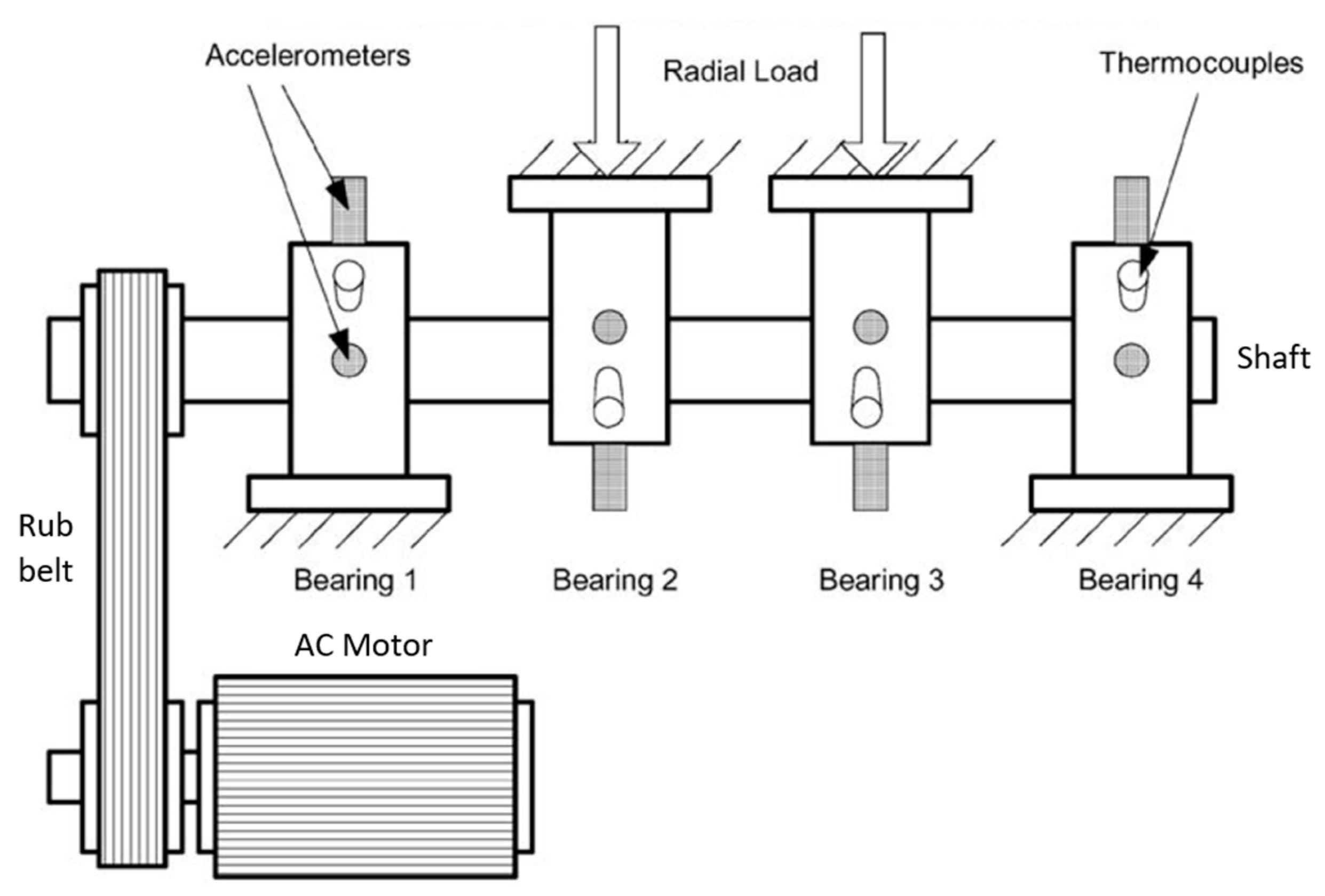
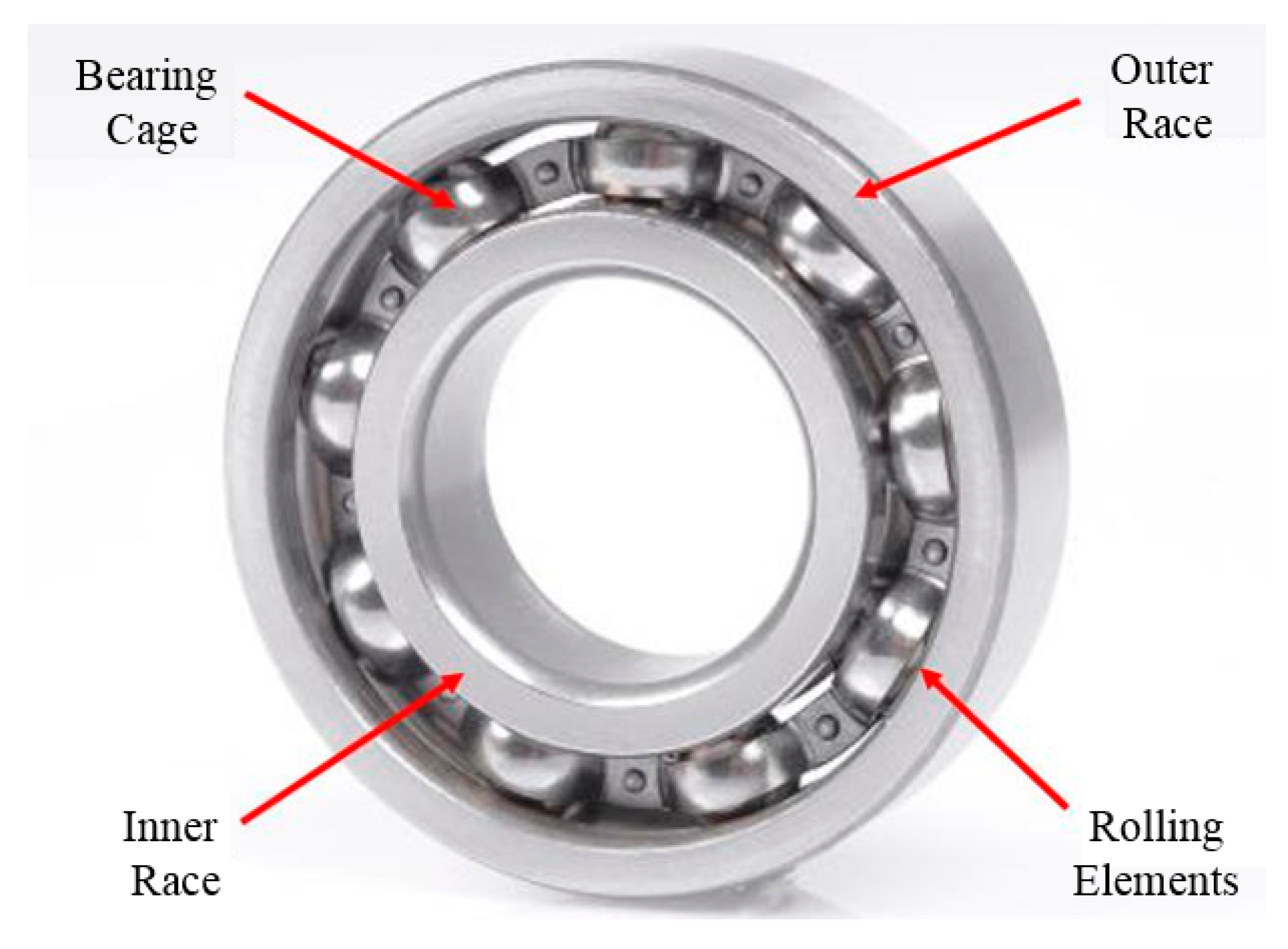
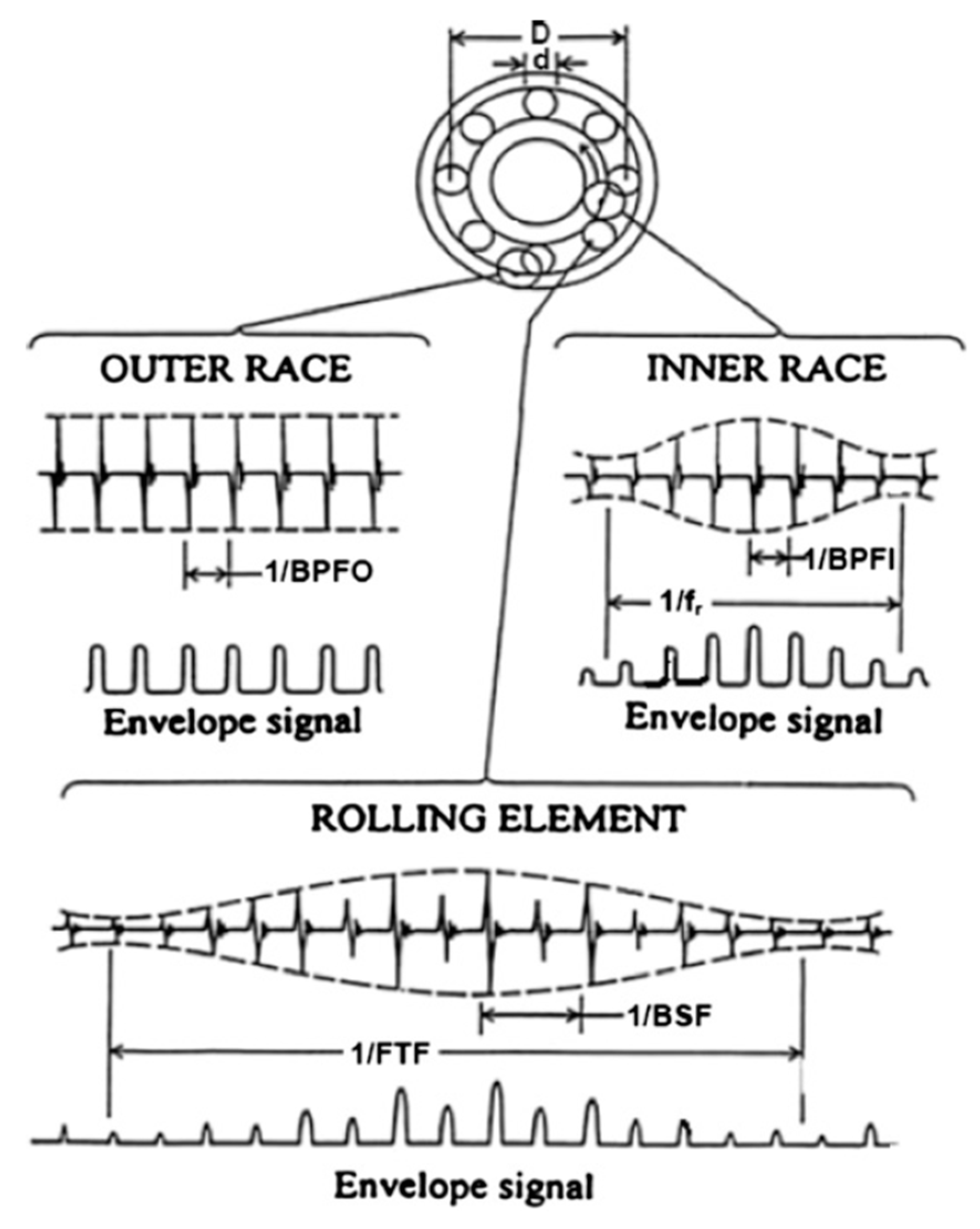
2.1. Description of IMS Dataset 1

As already mentioned, the signals that will be analyzed come from an open-access dataset released in 2014 by the NASA Center for Intelligent Maintenance Systems (IMS) [33]; the focus is on the results of the first of three run-to-failure experimental campaigns carried out at the University of Cincinnati, OH, USA, with support from Rexnord Corp., Milwaukee, MI, USA.

The test rig included four rolling bearings installed on a common shaft, set in rotation at a constant speed of 2000 RPM by an AC motor coupled to the shaft via rub belts (Figure 1). The four double row bearings were of type Rexnord ZA-2115, force-lubricated by a circulation system that regulated the flow and the temperature and charged with a 26,690 N (6000 lbs) constant radial load applied by a spring mechanism. Eight PCB 353B33 High-Sensitivity Quartz ICP accelerometers were installed on the bearing housing (two sensors for each bearing, mounted orthogonally along the x and y axes), and the sampling frequency was set to 20,480 Hz. The dataset consists of individual files that are 1 s vibration signal snapshots recorded at specific intervals, every 5 (for the first 54 acquisitions) or 10 min, but it is sometimes subjected to a series of interruptions that make the time history not continuous (Figure 2).

The experiment was stopped conventionally when the accumulation of debris on a magnetic plug exceeded a certain level, indicating the possibility of an impending failure. The resulting endurance duration was equal to 49,680 min (i.e., 34 days and 12 h), exceeding the bearing designed lifetime, which was more than 100 million revolutions.

The most relevant experimental set-up characteristics and findings of IMS dataset 1 are reported in

Table 1. Experimental set-up characteristics and findings of IMS dataset 1 (from [33]).

Start-stop time and date	From 22 October 2003 at 12:06:24 p.m. To 25 November 2003 at 11:39:56 p.m.
Entire experiment timespan	49,680 min (34 days and 12 h)
Effective data acquisition duration	36 min
Number of files	2156
Number of channels (accelerometers)	8
Channel arrangement	Bearing 1: channels 1 and 2 Bearing 2: channels 3 and 4 Bearing 3: channels 5 and 6 Bearing 4: channels 7 and 8
File recording interval	10 min (5 min for the first 43 files)
Location of detected faults at the end of the experiment	Bearing 3: inner race Bearing 4: rolling element and outer race

. It should be stressed that this dataset is particularly valuable because the bearing degradation was left to evolve naturally and was not artificially induced, as may often happen to speed up the experimental test.

Vibrational data collection was conducted with the National Instruments LabVIEW program thanks to a NI DAQ Card-6062E data acquisition, and the analysis that will be presented in this paper was developed with the software platform MATLAB 2021b by The MathWorks [34].

Considering the rolling bearing mechanical characteristics and working conditions of Table 2, it is possible to compute the value of the characteristic frequencies of the faults they are typically subjected to during their operating life, i.e., the fault signatures, by using the following formulas [1]:

$$\mathrm{BPFO}=\frac{n{f}_r}{2}\left(1-\frac{d}{D}\cos \varphi \right)$$

(1)

$$\mathrm{BPFI}=\frac{n{f}_r}{2}\left(1+\frac{d}{D}\cos \varphi \right)$$

(2)

$$\mathrm{FTF}=\frac{f_r}{2}\left(1-\frac{d}{D}\cos \varphi \right)$$

(3)

$$\mathrm{BSF}=\frac{f_{r}D}{2d}\left[1-{\left(\frac{d}{D}\cos \varphi \right)}^2\right]$$

(4)

where:

• $\mathrm{BPFO}\left(BallPassFrequency,OuterRace\right)$ is the frequency representing the fault signature on the outer race;
• $\mathrm{BPFI}\left(BallPassFrequency,InnerRace\right)$ is the frequency representing the fault signature on the inner race;
• $\mathrm{FTF}\left(FundamentalTrainFrequency\right)$ is the frequency representing the fault signature on the bearing cage;
• $\mathrm{BSF}\left(BallSpinFrequency\right)$ is the frequency representing the fault signature on the rolling element.

See the rolling element bearing of Figure 3.

Table 2. Rolling bearing mechanical characteristics and working conditions (from [33]).

Model	Rexnord ZA-2115
Pitch diameter D	71.5 mm (2.815 inch)
Rolling element diameter d	8.4 mm (0.331 inch)
Number of rolling elements per row n	16
Load contact angle ϕ	15.17°
Static load Q	26,690 N (6000 lbs.)
Shaft angular velocity ω	2000 rpm

Table 2. Rolling bearing mechanical characteristics and working conditions (from [33]).

Model	Rexnord ZA-2115
Pitch diameter D	71.5 mm (2.815 inch)
Rolling element diameter d	8.4 mm (0.331 inch)
Number of rolling elements per row n	16
Load contact angle ϕ	15.17°
Static load Q	26,690 N (6000 lbs.)
Shaft angular velocity ω	2000 rpm

The nominal rotation frequency of the transmission shaft $f_r$ can be directly obtained from the working conditions:

$$f_r=\frac{\omega }{2\pi }=\frac{2000\mathrm{rpm}}{2\pi ·60\mathrm{s}/\min }=33.3\mathrm{Hz}$$

(5)

where the corresponding characteristic frequencies of the faults are reported in

Table 3. Characteristic frequencies of the IMS test rig (from [33]).

Nominal rotation frequency of the shaft	33.3 Hz
Ball Pass Frequency Outer Race (BPFO)	236 Hz
Ball Pass Frequency Inner Race (BPFI)	297 Hz
Ball Spin Frequency (BSF)	278 Hz (2 × 139 Hz)
Fundamental Train Frequency (FTF)	15 Hz

.

2.2. Signal Analysis Techniques

In this Section, a list and a brief mathematical introduction of the diagnostic techniques used to analyze vibration signals are provided.

Techniques are divided into the three main phases of the condition monitoring process, i.e., fault detection, fault diagnosis and fault prognosis.

Moreover, within the fault diagnosis techniques, signal denoising techniques, filters and cyclostationary techniques are considered.

Fault detection techniques:

• Mean;
• Variance;
• Standard Deviation;
• Pea;
• Root Mean Squared value (RMS);
• Skewness;
• Crest Facto;
• Clearance Factor;
• Shape Factor;
• Impulse Factor;
• Peak-to-Peak;
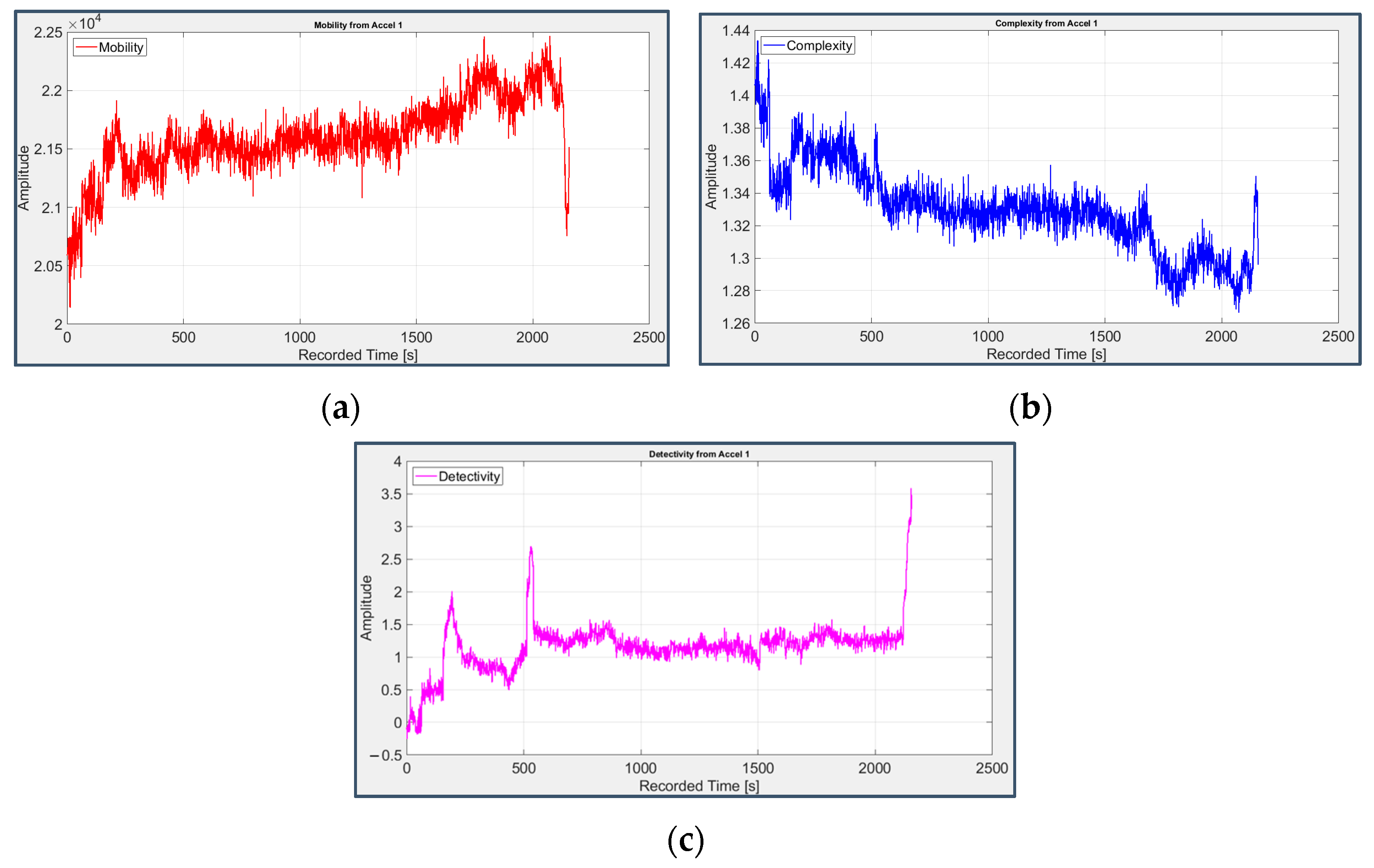
• Hjorth’s Parameters;
• Detectivity.

Fault diagnosis techniques:

• Short-Time Fourier Transform (STFT);
• Power Spectral Density (PSD);
• Squared Envelope Spectrum (SES);
• Autoregressive Linear Prediction (ALP);
• Time-Synchronous Averaging (TSA);
• Kurtosis (time domain);
• Kurtogram.

Signal denoising techniques:

• Daubechies’ Wavelets;
• Cepstrum Pre-Whitening (CPW).
• Filters:
• FIR;
• Adaptive.

Cyclostationary techniques:

• Spectral Correlation (SC);
• Cyclic Spectral Coherence (CSC);
• Improved Envelope Spectrum (IES);
• Wigner–Ville Distribution (WVD).

Fault prognosis techniques:

• Correlation;
• Monotonicity;
• Robustness.

The use of numerous statistical parameters is due to their limited analytical and computational complexity and their general and intuitive meaning for detection purposes, although they just play the role of high-level indicators and need to be followed by more in-depth, specific and elaborate techniques.

Table 4. Statistical parameters.

Parameter	Abbrev.	Formula
Mean	Mean	$\frac{\sum X}{N}$
Variance	Var	$\frac{\sum {\left(X-\overline{X}\right)}^2}{N-1}$
Standard Deviation	STD	$\sqrt{\mathrm{Var}}$
Root Mean Squared Value	RMS	$\sqrt{\frac{\sum X^2}{N}}$
Skewness	Skew	$\frac{\frac{1}{N}\sum {\left(X-\overline{X}\right)}^3}{\mathrm{ST}{\mathrm{D}}^3}$
Kurtosis	Kurt	$\frac{\frac{1}{N}\sum {\left(X-\overline{X}\right)}^4}{\mathrm{ST}{\mathrm{D}}^4}$
Peak	Peak	$\mathrm{Max}\left(\left|X\right|\right)$
Crest Factor	CF	$\frac{\mathrm{Peak}}{\mathrm{RMS}}$
Clearance Factor	CL	$\frac{\mathrm{Peak}}{{\left(\frac{\sum \sqrt{X}}{N}\right)}^2}$
Shape Factor	SF	$\frac{\mathrm{RMS}}{\mathrm{Mean}}$
Impulse Factor	IF	$\frac{\mathrm{Peak}}{\mathrm{Mean}}$
Peak-to-Peak	P2P	$\mathrm{Max}\left(X\right)-\mathrm{Min}\left(X\right)$

shows the mathematical definition of the most common statistical parameters.

Hjorth’s parameters and Detectivity are statistical time-domain quantities, but their application in the context of signal diagnosis is still unusual. The formers (Activity, Mobility, Complexity) were introduced by Hjorth and Elema-Schönander in 1970 and are commonly used in the analysis of electroencephalography (EEG) signals for feature extraction [35] and in the tactile signal analysis in the robotic area [36]. They are related to the variance of the signal and of its subsequent derivatives, and can be computed with minimum effort and resources, suggesting their use in real-time application for the condition monitoring of ball bearings or as a feature array for Machine Learning techniques.

The “Activity” of a vibration signal ($\mathrm{Act}\left(x\right)$) is defined as the variance of its amplitude, and therefore it has the same dimension of the signal (the one of the accelerations in the current case) and it is directly related to its power.

“Mobility” ($\mathrm{Mob}\left(x\right)$) is related to the variance of the vibration signal velocity, so it is associated to the jerk (first time derivative of the signal) and its dimension is expressed as a ratio per time unit.

“Complexity” ($\mathrm{Com}\left(x\right)$) is a dimensionless parameter, connected to the variance of the acceleration of the signal, hence to the snap (second time derivative of the signal and four-time derivative of space).

Moreover, these three parameters can be also derived in the frequency domain, starting from the spectral moments $m_n$ of the time signal $x\left(t\right)$ [36]:

$$\mathrm{Act}\left(x\right)={\sigma }^2\left(x\right)=\underset{T\to \infty }{\lim }\frac{1}{T}{{\displaystyle \int }}_0^T{x}^2\left(t\right)dt=m_0={{\displaystyle \int }}_{-\infty }^{+\infty }S\left(\omega \right)d\omega {\left[\mathrm{m}/{\mathrm{s}}^2\right]}^2$$

(6)

$$\mathrm{Mob}\left(x\right)=\sqrt{\frac{\mathrm{Act}\left(\dot{x}\right)}{\mathrm{Act}\left(x\right)}}=\sqrt{\frac{m_2}{m_0} } \left[{\mathrm{t}}^{-1}\right]$$

(7)

$$\mathrm{Com}\left(x\right)=\sqrt{\frac{\mathrm{Mob}\left(\dot{x}\right)}{\mathrm{Mob}\left(x\right)}}=\sqrt{\frac{m_4/m_2}{m_2/m_0} } \left[ \right]$$

(8)

where $S\left(\omega \right)$ is the power spectral function, defined as the product of the Fourier transform $F\left(\omega \right)$ and its complex conjugate function $F^{*}\left(\omega \right)$:

$$S\left(\omega \right)=F\left(\omega \right)·F^{*}\left(\omega \right)={{\displaystyle \int }}_{-\infty }^{+\infty }x\left(t\right)·x^{*}\left(t\right)dt$$

(9)

and the generic spectral moment of order $n$ can be computed in the form:

$$m_n=F\left(\omega \right)·F^{*}\left(\omega \right)={{\displaystyle \int }}_{-\infty }^{+\infty }{\omega }^n·S\left(\omega \right)d\omega$$

(10)

As for their interpretation in the field of predictive maintenance, Activity and Complexity are proportional to the amplitude of the fault frequency components, while Mobility is expected to reduce with fault progression.

In order to sum up the informative contribution of Hjorth’s parameters into a single value, another quantity, called Detectivity ($\mathrm{Detect}$), was introduced in [37] and defined as:

$$\mathrm{Detect}={\mathrm{Act}}_{\left(dB\right)}-{\mathrm{Mob}}_{\left(dB\right)}+{\mathrm{Com}}_{\left(dB\right)}$$

(11)

where:

$${\mathrm{Act}}_{\left(dB\right)}=10·{\log }_{10}\left(\frac{\mathrm{Act}}{{\mathrm{Act}}_{\mathrm{ref}}}\right)$$

(12)

$${\mathrm{Mob}}_{\left(dB\right)}=10·{\log }_{10}\left(\frac{\mathrm{Mob}}{{\mathrm{Mob}}_{\mathrm{ref}}}\right)$$

(13)

$${\mathrm{Com}}_{\left(dB\right)}=10·{\log }_{10}\left(\frac{\mathrm{Com}}{{\mathrm{Com}}_{\mathrm{ref}}}\right)$$

(14)

The three terms in the right member of (11) are expressed in Decibel, after being normalized by computing the ratio between their value on the signal to be diagnosed and a reference value coming from their application to the data collected on the faultless component. Mobility behaves as an attenuator due to its inverse trend with respect to the evolution of the fault, while Activity and Complexity behave as amplifiers.

Due to the particular nature of the vibration signals produced by damaged rolling bearings, which are classified as quasi-pseudo-cyclostationary of the second order, it is convenient to use dedicated techniques, specifically formulated for their treatment. As previously anticipated, four powerful and complex cyclostationary techniques have been employed for the analysis of the dataset: (i) Spectral Correlation $S_{2x}\left(\alpha ,f\right)$, defined in the spectral frequency ($f$)–cyclic frequency ($\alpha$) domain as the bidimensional Fourier transform of the Instantaneous Autocorrelation Function $R_{2x}\left(t,\tau \right)$; (ii) Cyclic Spectral Coherence ${\mathrm{CSC}\mathrm{oh}}_{2x}\left(\alpha ,f\right)$, which is a normalized version of the previous technique; (iii) Improved Envelope Spectrum ${\mathrm{IES}}_{\mathrm{CSC}\mathrm{oh}}\left(\alpha \right)$, obtained as the integral of ${\mathrm{CSC}\mathrm{oh}}_{2x}$ computed on a limited spectral frequency band $\left[F_1,F_2\right]$, providing information similar to that provided by the traditional envelope analysis but from a different and unconventional perspective; and iv) Wigner–Ville Distribution ${\mathrm{WVD}}_{2x}\left(t,f,\varphi \right)$, belonging to the class of the time-frequency domain techniques [38]:

$$S_{2x}\left(\alpha ,f\right)=F{T}_{t\to \alpha }F{T}_{\tau \to f}\left\{R_{2x}\left(t,\tau \right)\right\}$$

(15)

$${\mathrm{CSC}\mathrm{oh}}_{2x}\left(\alpha ,f\right)=\frac{S_{2x}\left(\alpha ,f\right)}{\sqrt{S_{2x}\left(0,f\right)S_{2x}\left(0,f-\alpha \right)}}$$

(16)

$${\mathrm{IES}}_{\mathrm{CSC}\mathrm{oh}}\left(\alpha \right)=\frac{1}{F_2-F_1}{{\displaystyle \int }}_{F_1}^{F_2}\left|{\mathrm{CSC}\mathrm{oh}}_{2x}\left(\alpha ,f\right)\right|df$$

(17)

$${\mathrm{WVD}}_{2x}\left(t,f,\varphi \right)=F{T}_{\tau \to f}\left\{R{s}_{2x}\left(t,\tau \right)\right\}$$

(18)

where:

$$R{s}_{2x}\left(t,\tau \right)={{\displaystyle \int }}_{-\infty }^{+\infty }x\left(u+\tau /2\right)x^{*}\left(u-\tau /2\right)\varphi \left(t-u,\tau \right)du$$

(19)

As for fault prognosis, the suitability of the statistical parameters (excluding Hjorth’s ones) as metrics exploitable for predicting future signal trends, namely the so-called “health indicators” (or “health indexes”—HI), was assessed with the computation of the prognostic values of Correlation ($\mathrm{Corr}$), Monotonicity ($\mathrm{Mon}$) and Robustness ($\mathrm{Rob}$), defined as [20]:

$$\mathrm{Corr}\left(T,X\right)=\frac{\mathrm{Cov}\left(T,X\right)}{{\sigma }_T{\sigma }_X}$$

(20)

$$\mathrm{Mon}\left(T,X\right)=\frac{\mathrm{Cov}\left(r_T,r_X\right)}{{\sigma }_{r_T}{\sigma }_{r_X}}$$

(21)

$$\mathrm{Rob}\left(T,X\right)=\frac{1}{k}{\displaystyle \sum }_{k}exp\left(-\left|\frac{X\left(k\right)-\tilde{X}\left(k\right)}{X\left(k\right)}\right|\right)$$

(22)

in which $X$ is the evaluated quantity (as a statistical parameter), $T$ is the time domain, $\mathrm{Cov}$ is the covariance, $r$ represents the rank of a vector, composed by the positions of its elements according to a given sorting, and $˜$ is the symbol of the smooth value, obtained with the use of a moving-average filter applied on all the $k-1$ elements before the $k$-th one.

Specifically, Correlation (aka Pearson’s Correlation) measures the linearity between $X$ and $T$ and is expressed by a number included in the interval [−1, 1] (where 1 states perfect linearity), Monotonicity (aka Spearman Correlation) is defined on the same range and provides information about the continuity of the increasing or decreasing of the quantity over time, and Robustness is related to the amount of noise that affects the signal, and therefore its value is desirably as low as possible so not to compromise the prognostic ability of the parameter.

3. Results

In this Section, the diagnostic results derived from the application of the aforementioned techniques to the considered dataset will be presented. To avoid redundancy, only the more meaningful elaborated signals between those coming from the couple of orthogonal sensors mounted on each bearing will be considered.

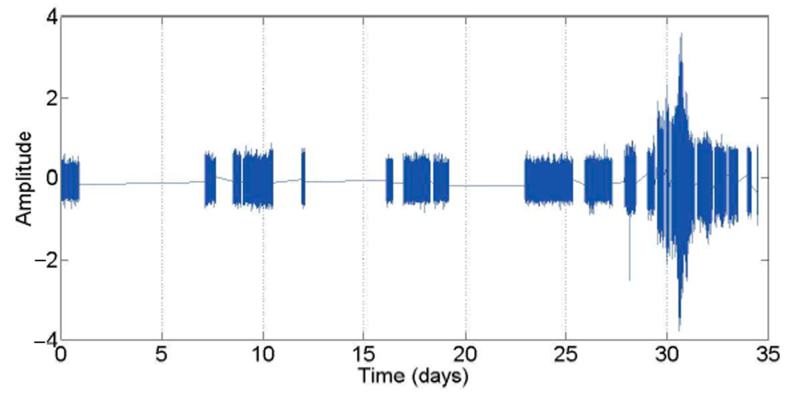
3.1. Fault Detection

The computation of statistical parameters is of paramount importance to reveal the presence of an incoming fault, accomplishing the first phase of condition monitoring. In the following analyses, parameter calculation is performed on each set of 20,480 $\left(f_s\right)$ samples acquired for each second of testing, so that only one statistical value per second is obtained.

If a parameter trend is examined along the time duration of the whole registration (made continuous with the exclusion of the interruptions of acquisition occurring in real time), it can be observed that the Mean, Variance and Standard Deviation of bearings 1 and 2 (Figure 4a and Figure 5a) remain almost constant, with a slight increase just at the very end of the experiment, probably due to the propagation of vibrations produced by other damaged bearings and detected by sensors 1 and 3 because of the physical continuity of the testing, in which all the components are installed on a single shaft. RMS value, Skewness and Kurtosis (Figure 4b–d and Figure 5b–d), albeit oscillating, do not exhibit a global monotonicity too, except for in the last measurements, for the reason just mentioned.

On the contrary, the presence of faults on bearings 3 and 4 can be clearly deduced from the RMS value (Figure 6b and Figure 7b) and even more from the Kurtosis (Figure 6d and Figure 7d), which starting from a value around 3, typical of a Gaussian distribution, raises over 70 from the 1831st second (31st day of test) for the third bearing and from the 1486th second (28th day of test) for the fourth one. Mean, Variance and Standard Deviation (Figure 6a and Figure 7a) remain mostly stable, and Skewness (Figure 6c and Figure 7c) does not show a clear reduction, as expected in the case of a fault.

Similar results can be obtained by considering advanced statistical parameters, i.e., Peak, Crest Factor, Clearance Factor, Shape Factor, Impulse Factor and Peak-to-Peak. On one hand, these parameters do not provide relevant information if applied to the signals from bearings 1 and 2 (Figure 8 and Figure 9). On the other hand, with respect to the vibration signals acquired from bearings 3 and 4, consistent information is provided by Clearance Factor (Figure 10a and Figure 11a) and Impulse Factor (Figure 10b and Figure 11b).

Figure 12, Figure 13, Figure 14 and Figure 15 display the trend of Hjorth’s parameters (omitting Activity, which is equivalent to Variance) and Detectivity; the latter has been computed using the first 5 days files (first 51 s of acquisition) to obtain the reference values involved in its formulation (11).

Their behavior agrees with that of the previous parameters: the Mobility (Figure 12a and Figure 13a) and Complexity (Figure 12b and Figure 13b) of bearings 1 and 2 have opposite trends than those that would be associated to a fault, while for bearings 3 and 4 Mobility slightly decreases (Figure 14a and Figure 15a) and Complexity increases (Figure 14b and Figure 15b).

However, Detectivity is the parameter that offers the clearest signature of fault with a significant increase in its value (Figure 14c and Figure 15c), proving its efficacy in the field of predictive maintenance as a combination (and an informative summa) of Hjorth’s parameters. The same temporal occurrence of faults previously deduced via statistical parameters is also observed considering Detectivity, with a quite-late fault on bearing 3 and an earlier one on bearing 4.

3.2. Fault Diagnosis

Beside pointing out the presence of faults, the phase of fault detection is essential to temporally locate their occurrence and then to identify the limited portion of signal to be analyzed in the second step of the study, which is fault diagnosis. This is based on the application of more complex techniques with higher computational effort to determine the exact nature of each fault, i.e., the particular bearing sub-component affected by it.

Since the statistical parameters previously adopted for the fault detection revealed the presence of faults only on bearings 3 and 4, and not on bearings 1 and 2, these last two bearings are not further considered, and the fault diagnosis is carried out only on bearings 3 and 4.

The signal from the last 49 s of acquisition, belonging to the last part of the 33rd and all the 34th day of the experiment, will be considered for bearing 3, as well as the signal from the 26th day until the end of the campaign for bearing 4, in light of the earlier occurrence of faults on it, which tend to gradually reduce their impact on the signal and their impulsive nature due to progressive smoothing of the damaged surfaces.

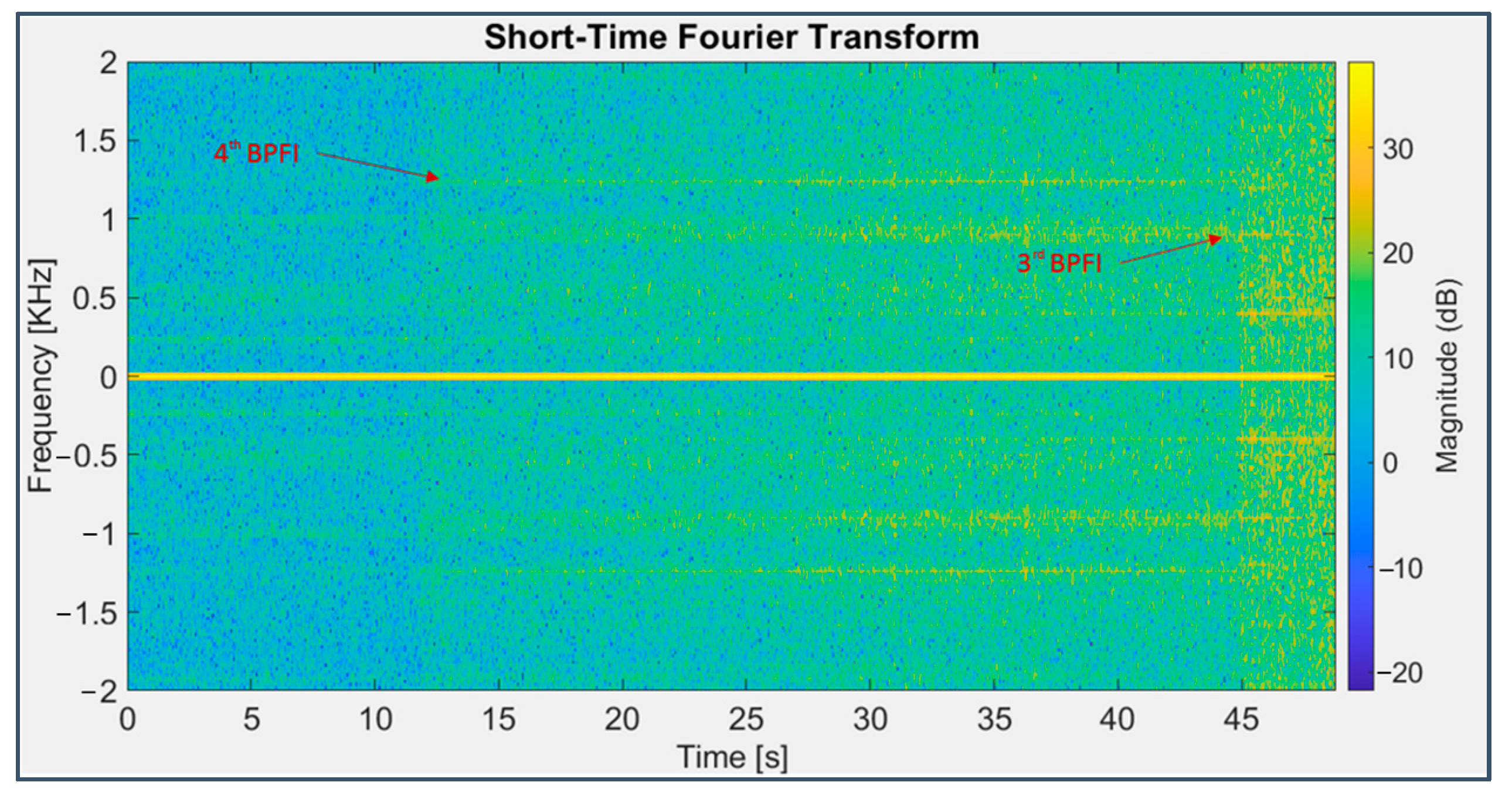
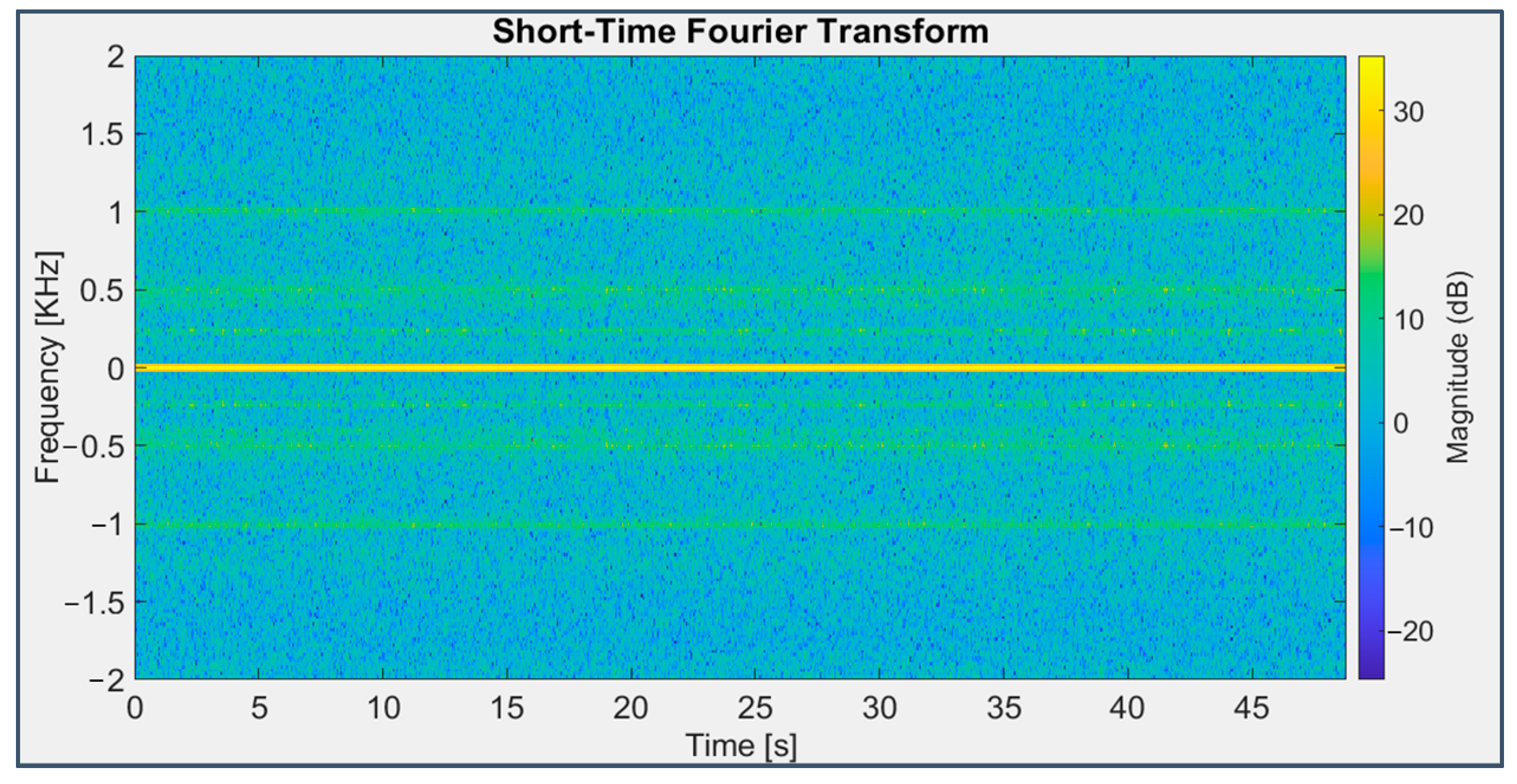
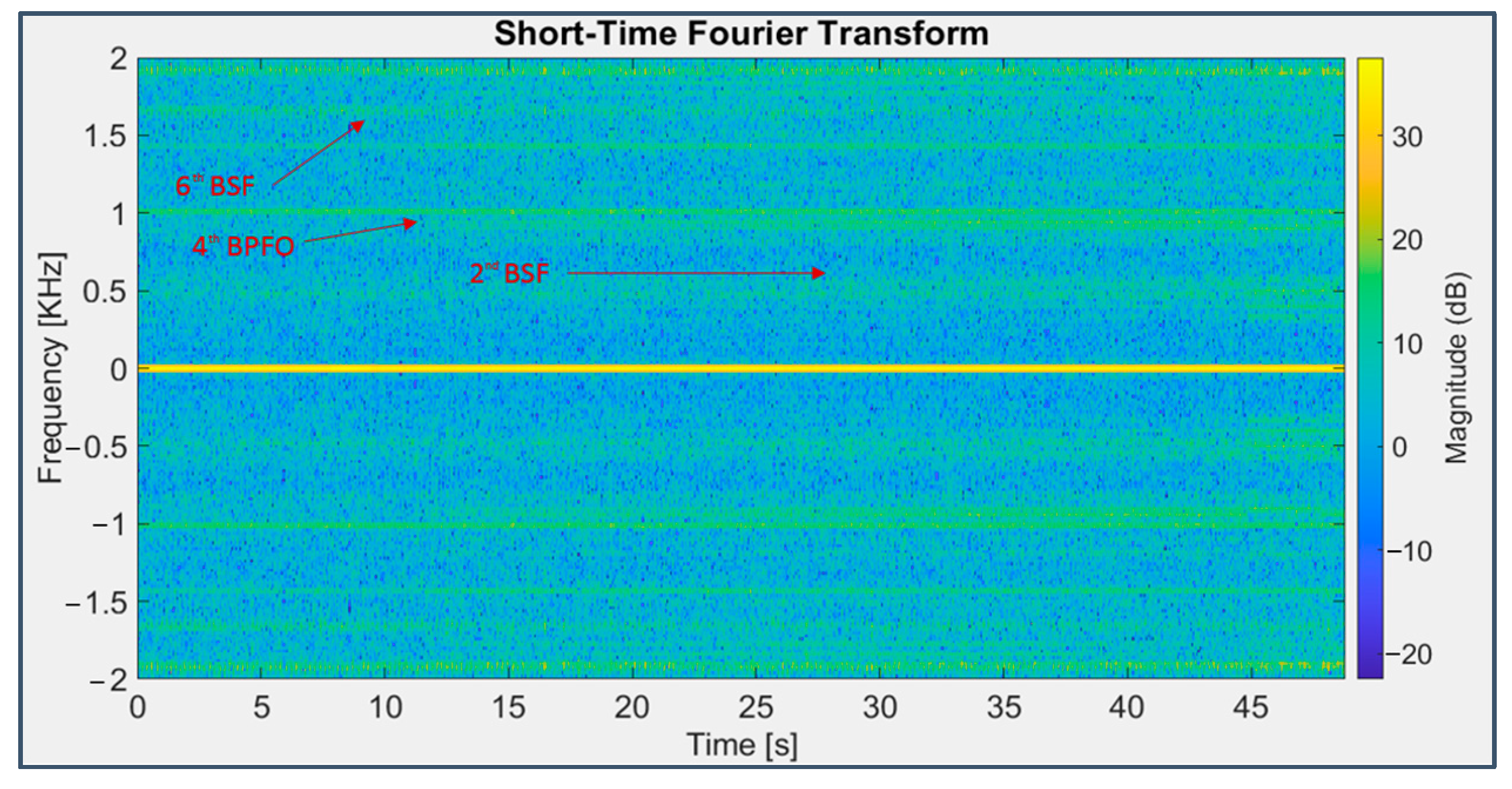
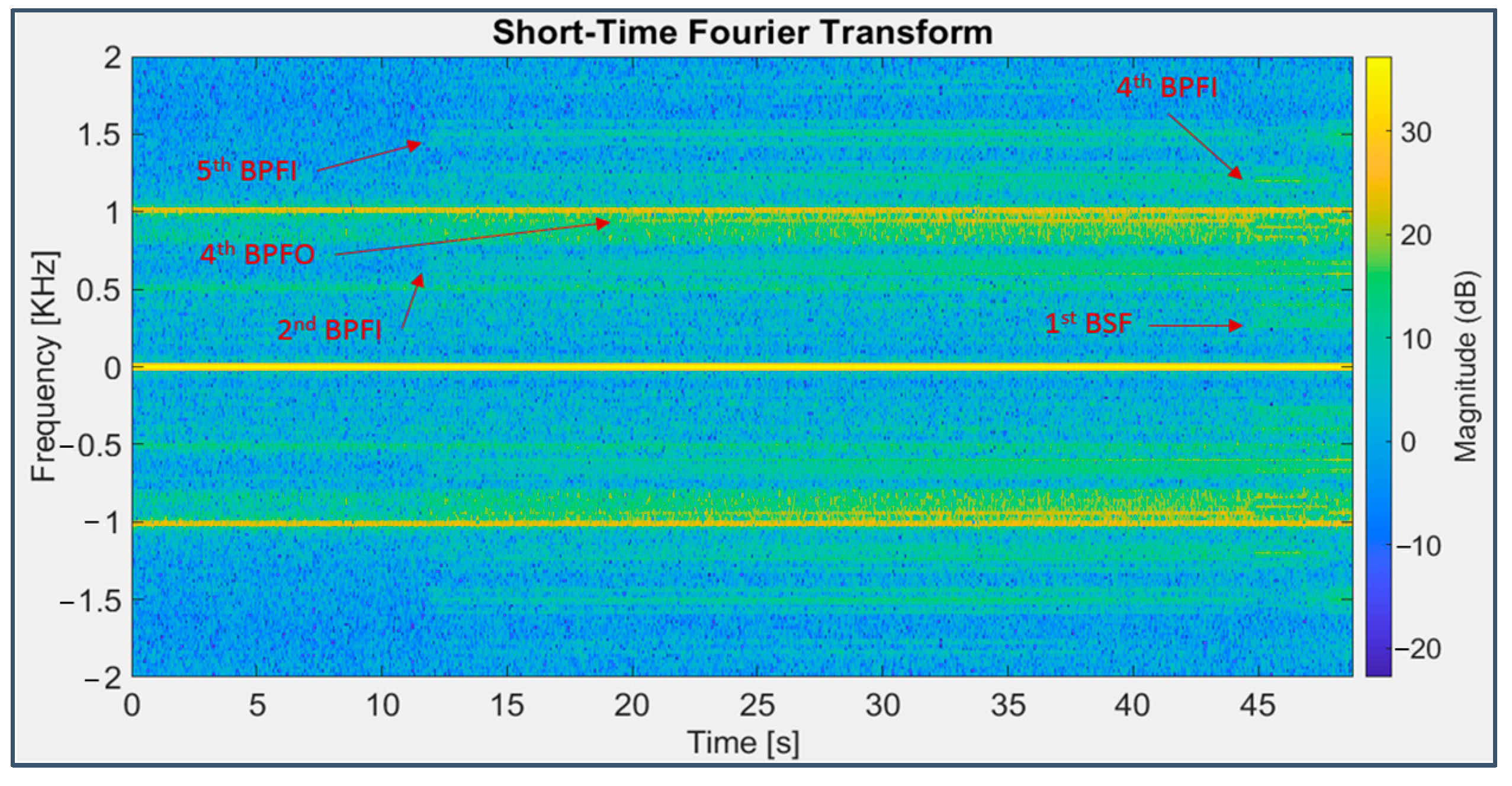
3.2.1. Short-Time Fourier Transform (STFT)

Before filtering the signal, it is advisable to study it in its raw version to prevent the loss of important information on account of a premature and inaccurate pre-treatment.

The first applied technique is the Short-Time Fourier Transform, defined on the time-frequency domain, assuming a Hamming window with a length equal to 1024 and without overlap, as suggested in [13].

It is possible to detect a general amplitude increase in the spectral components of bearing 3 starting from the 12th second (of the last 49 considered), even more evident beyond the 45th (Figure 16), with the appearance of the fourth and third harmonics of the BPFI (297 Hz), respectively, still completely invisible in the first days of screening (Figure 17); in the chromatic graph related to bearing 4’s signal (Figure 18), a clear display of the fourth harmonic of the BPFO is detectable (although considering 238 Hz instead of 236 Hz, probably because of slipping among parts) as well as the presence of the second and sixth harmonics of the BSF (278 Hz). It is worth noting that traces of the same harmonic series are visible even in the signal acquired by the third accelerometer on bearing 2 (Figure 19), especially those related to the fault occurring on bearing 3, which is contiguous to it on the shaft.

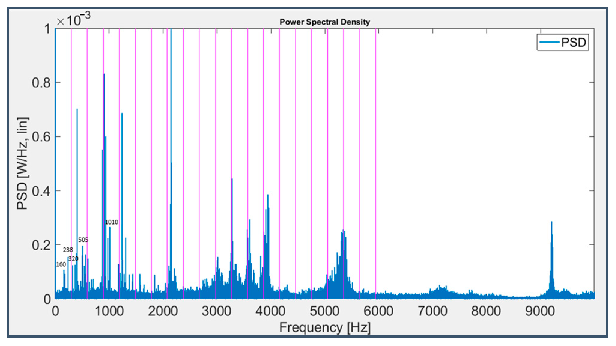
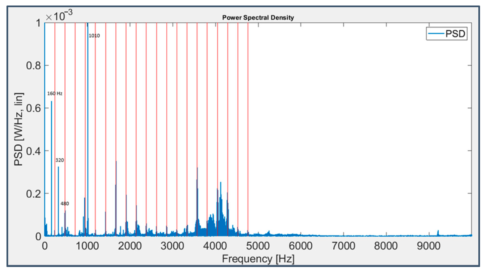
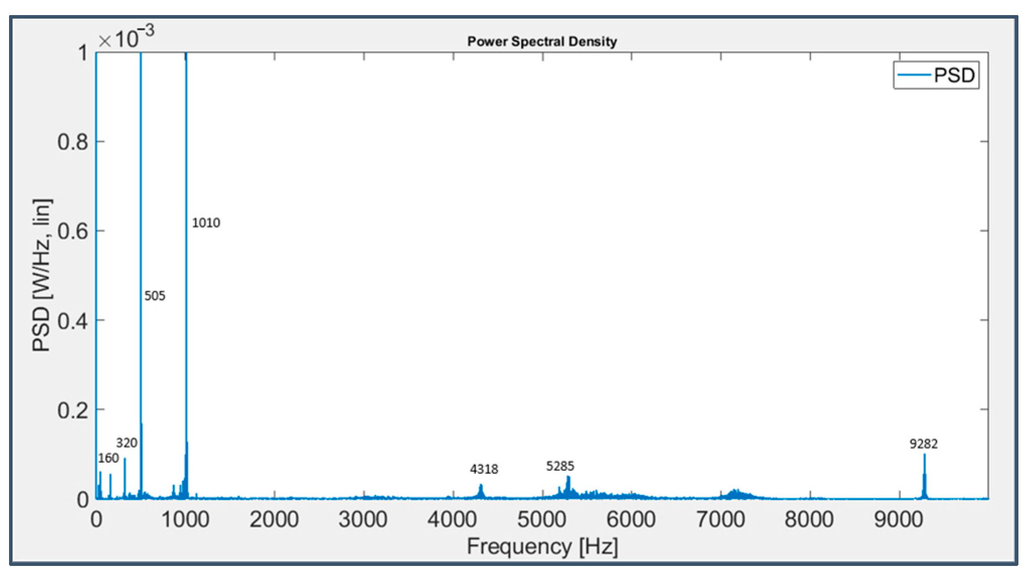
3.2.2. Power Spectral Density (PSD)

Starting again from the raw signal, the Power Spectral Density technique has been applied, obtaining information about the frequency distribution of the signal power; its formulation implies the computation of the signal Fourier transform, the corresponding square (power), the division of the result by the sampling frequency $f_s$ and the number of sampled values $N$ (density), a chain of operations that may be equivalently replaced by the evaluation of the periodogram:

$$PSD\left(f\right)=\frac{1}{f_s·N}{\left|{\displaystyle \sum }_{n=0}^{N-1}{x}_n{e}^{-j2\pi f \Delta t n}\right|}^2 with -\frac{1}{2}\Delta t\le f\le \frac{1}{2}\Delta t, \Delta t=\frac{1}{f_s}$$

(23)

In the graphs, shown in linear scale for purposes of clarity, some harmonics of the BPFI for bearing 3 (Figure 20, with harmonics highlighted in magenta) and of the BPFO for bearing 4 (Figure 21, with harmonics highlighted in red as multiples of 238 Hz instead of 236 Hz, as stated before) are already visible, but their detection is strongly affected by the emergence of other frequency lines related to the test rig mechanical structure and hence still present at the beginning of the experiment (Figure 22); specifically, they are located at 160 Hz and their harmonic frequencies (320 Hz and 480 Hz) and at 505 Hz and its striking double (1011 Hz). There are also peaks at very high frequencies, around 4000–5000 Hz and 9000 Hz, probably related to the system natural resonances. It is curious to observe that the first harmonic of the BPFO is more clearly visible in the spectrum of bearing 3 than in that of bearing 4 due to the cross-talk among contiguous sensors.

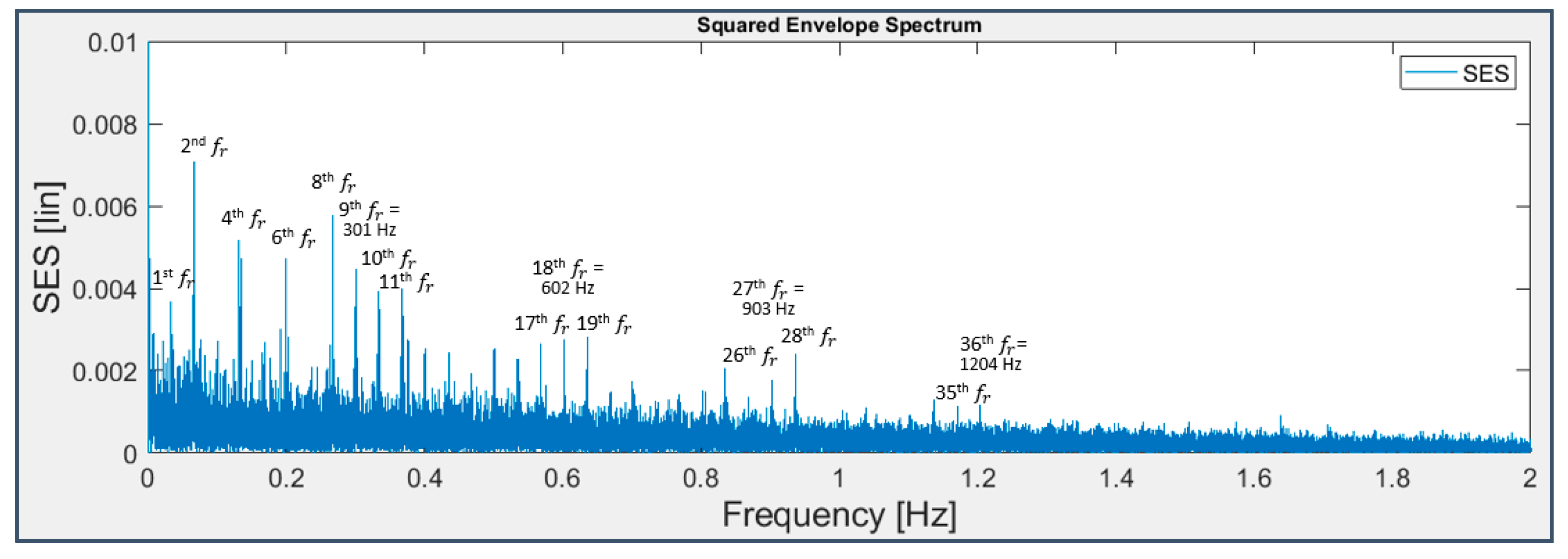
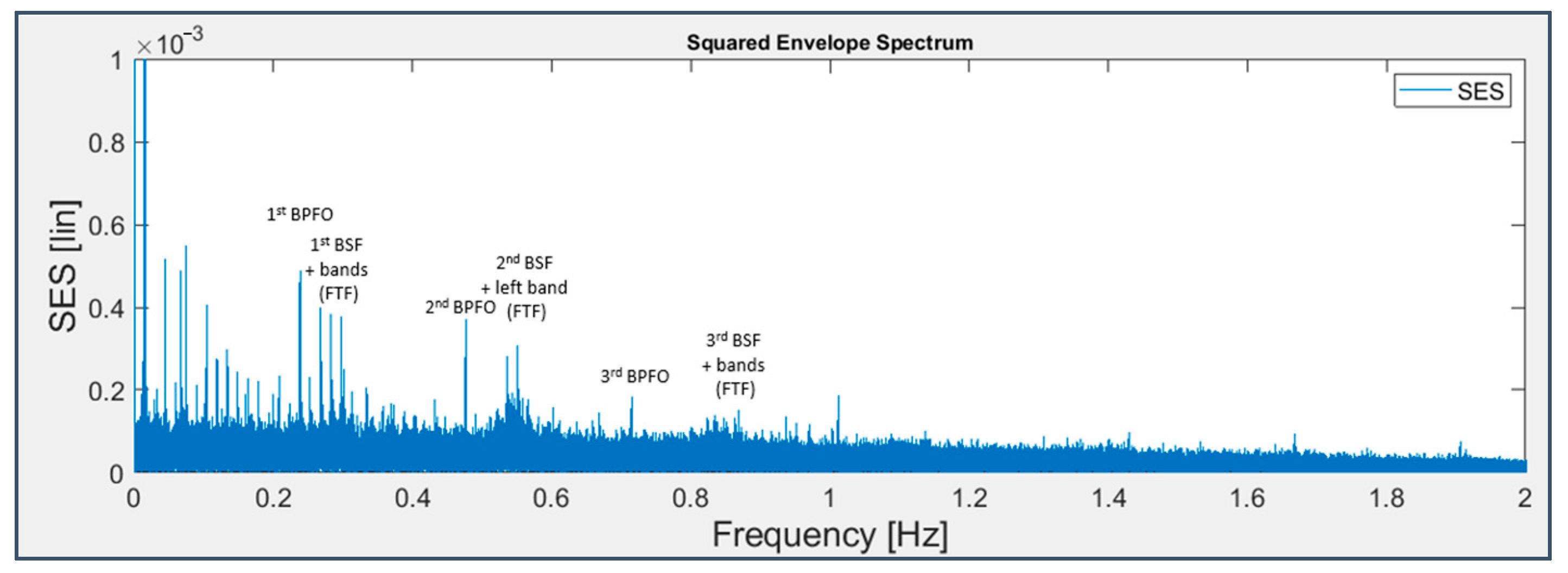
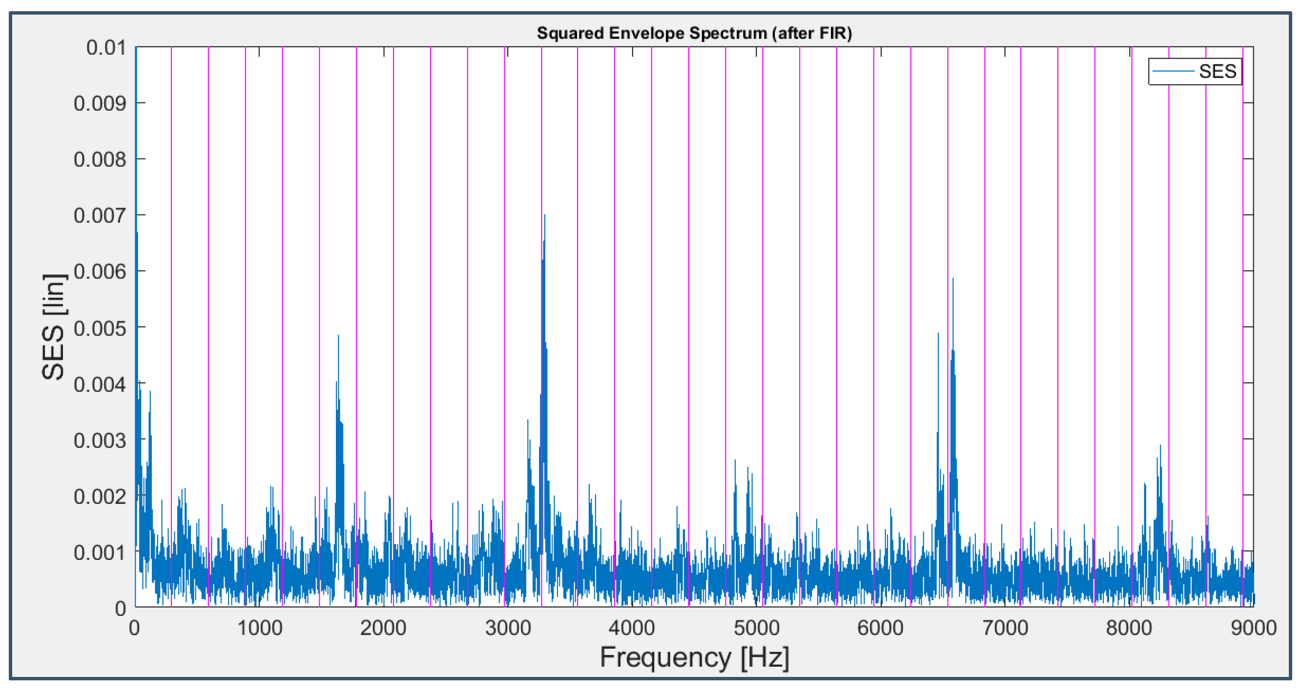
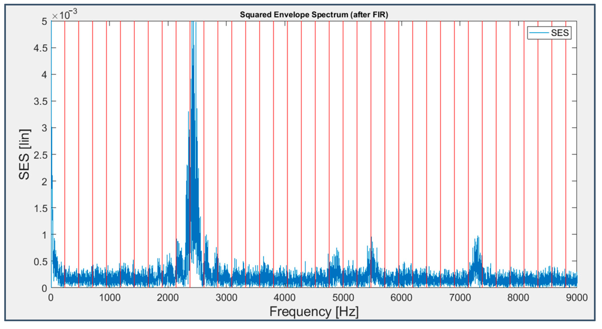
3.2.3. Squared Envelope Spectrum (SES)

The Squared Envelope Spectrum is considered a benchmark among the diagnostic techniques and it is attained through signal demodulation, firstly filtering the signal (in the case under examination, with a low-pass filter with cut-off frequency equal to $f_s$/16 = 1280 Hz), and then obtaining the analytic signal with the Hilbert transform before finally computing the envelope signal as the absolute value of the analytic one and applying the Fourier transform to return to the frequency domain.

It is known from the literature that squaring the signal at the very beginning of this process (i.e., correlating the signal with itself) is beneficial because it emphasizes the modulation and the clarity of information detectable in the final spectrum (while a squaring in the frequency domain would harmfully blur it). This operation is conveniently introduced for the considered dataset, which is characterized by inner race and rolling element faults, typically modulated by shaft rotation frequency $f_r$ and cage frequency FTF, respectively (Figure 23); as a matter of fact, in Figure 24 and Figure 25 the BPFI and BSF harmonics are accompanied by the characteristic modulation sidebands.

Specifically, in Figure 24, regarding bearing 3, the even harmonics of the shaft rotation frequency appear distinctly, while the odd ones emerge from noise only when near to the BPFI harmonics, as their sidebands.

Truthfully, the BPFI harmonics are not present directly, but indirectly, through the excitation exerted on those of shaft rotation; namely, the spectrum shows frequency lines at 301 Hz and 602 Hz, multiples of $f_r$ = 33.3 Hz, rather than at 297 Hz and 594 Hz, fundamental and second harmonic frequencies of the BPFI; in spite of the closeness of these values, their difference is not negligible or imputable to a mere approximation.

In Figure 25, about bearing 4, at least the first three harmonics of the BPFO can be detected, not subjected to modulation effects, and so can those of the BSF (centered on the multiple frequencies of 282 Hz instead of the nominal 278 Hz) with sidebands distant from the fault frequencies by the cage frequency, with the left band higher than the right one, unlike the theoretical case (Figure 23).

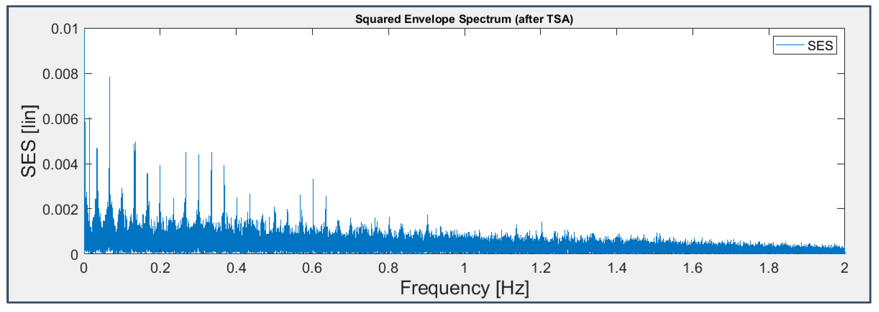
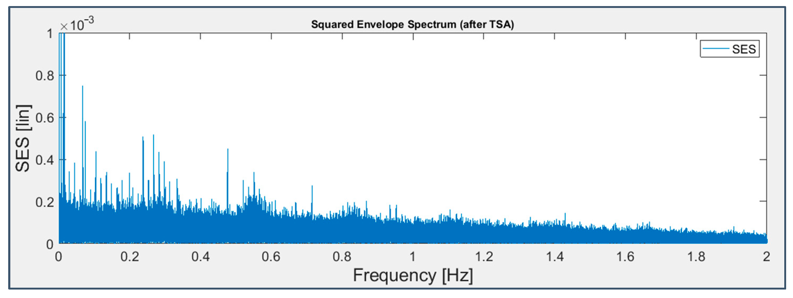
3.2.4. Time-Synchronous Average (TSA)

While fault frequency components have already been recognized thanks to the techniques applied so far, in order to accomplish a comprehensive and detailed study it is necessary to consider pre-processing techniques with the aim of denoising and filtering the raw signal to remove the presence of noise and masking components unrelated to faults, such as the harmonic series of the frequencies at 160 Hz and 505 Hz, making fault signatures even more easy to detect.

The following techniques will be applied, re-starting each time from the original signal, and will be followed by the use of the SES to make a consistent comparison among their effect.

The Time-Synchronous Average is a common time-domain diagnostic tool used as a pre-treatment technique to remove the deterministic components from the signal, bringing to light in the residual part those connected to bearing faults, which are cyclostationary; for the signal under test, the average has been made on time intervals that are synchronous to the shaft rotation for bearing 3 and to the cage rotation for bearing 4. The resulting graphs (Figure 26 and Figure 27) are similar to those already obtained (Figure 24 and Figure 25, respectively), with no added information, making the technique not useful.

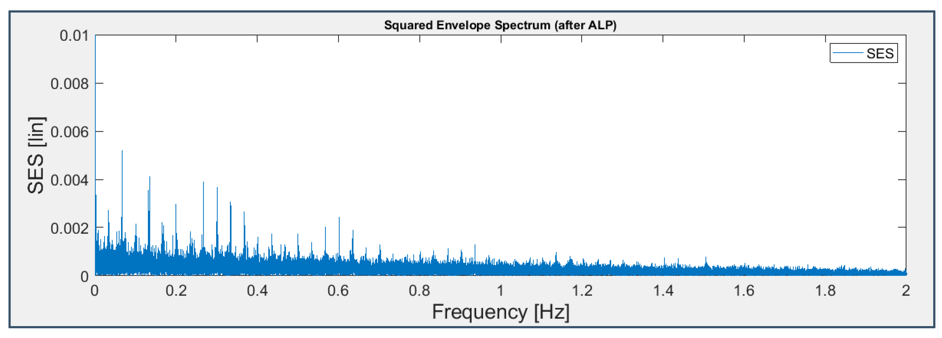
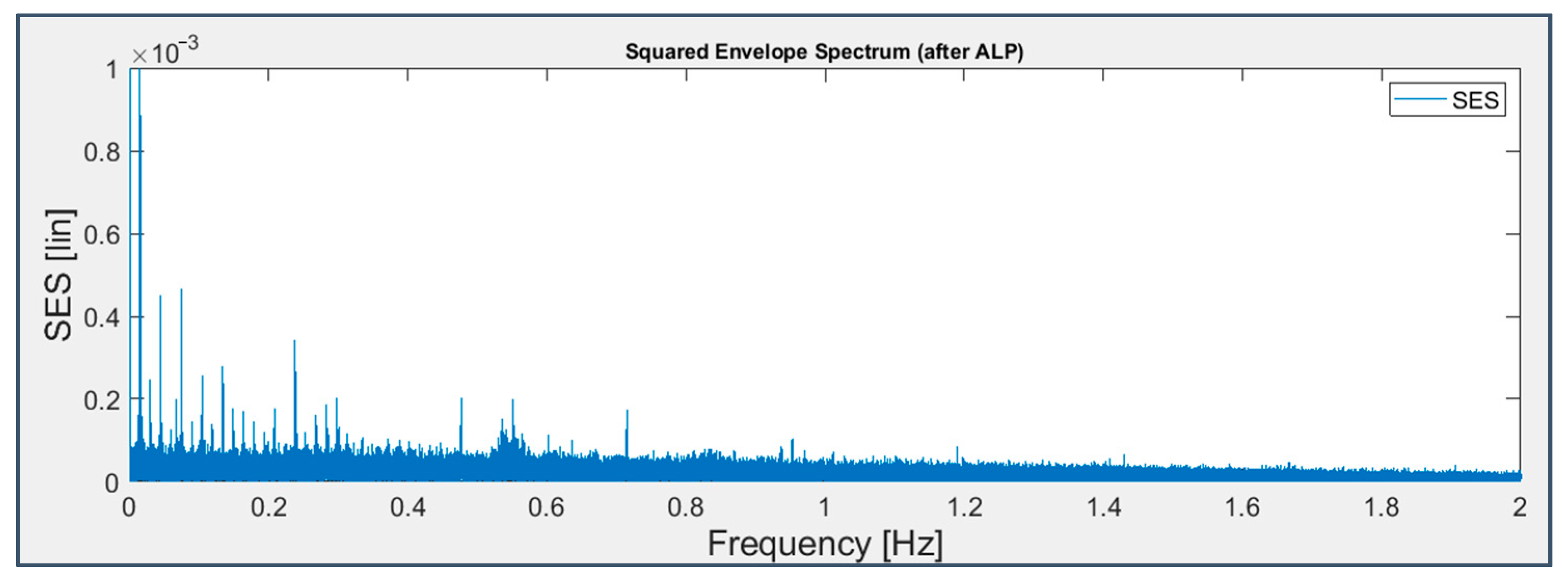
3.2.5. Autoregressive Linear Prediction (ALP)

According to the common practice, the Autoregressive Linear Prediction technique is used as a pre-whitening action and it implies at first obtaining the weighting coefficients of the fourth-order autoregressive model (with a form similar to that of a IIR filter), applying Yule–Walker equations and the Levinson–Durban recursive algorithm, then computing the prediction and finally deriving the residual signal as the difference between the initial and the predicted ones.

In the present case, ALP and SES techniques remove part of the background noise, but the improvement on the information content remains poor (Figure 28 and Figure 29).

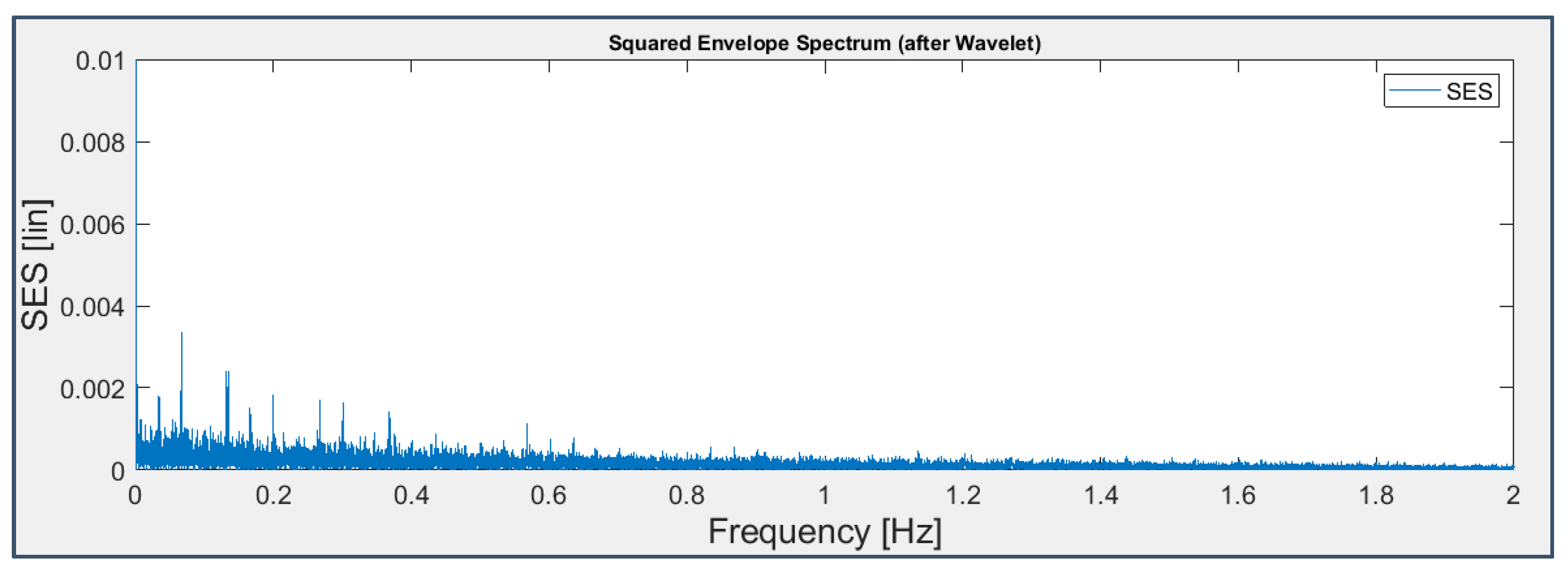
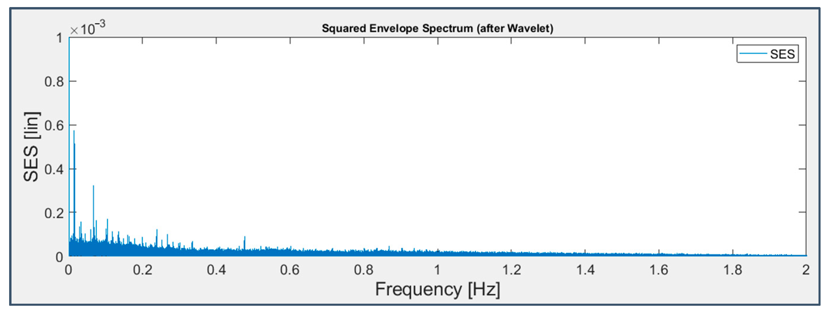
3.2.6. Daubechies’ Wavelets

A more advanced technique for denoising purposes is that based on the wavelets, a family of functions with a fixed shape, but which can be shifted and dilated in the time starting from the definition of a root function, i.e., the mother wavelet. Specifically, Daubechies’ orthogonal wavelets of the fifth level have been chosen, determining the extent and threshold values of the blocks with the James–Stein method.

The signal processed via Wavelets and SES techniques appears denoised and cleaned up from masking components (Figure 30 and Figure 31); however, the fault spectral lines, albeit visible, are not as emerging as would be desirable.

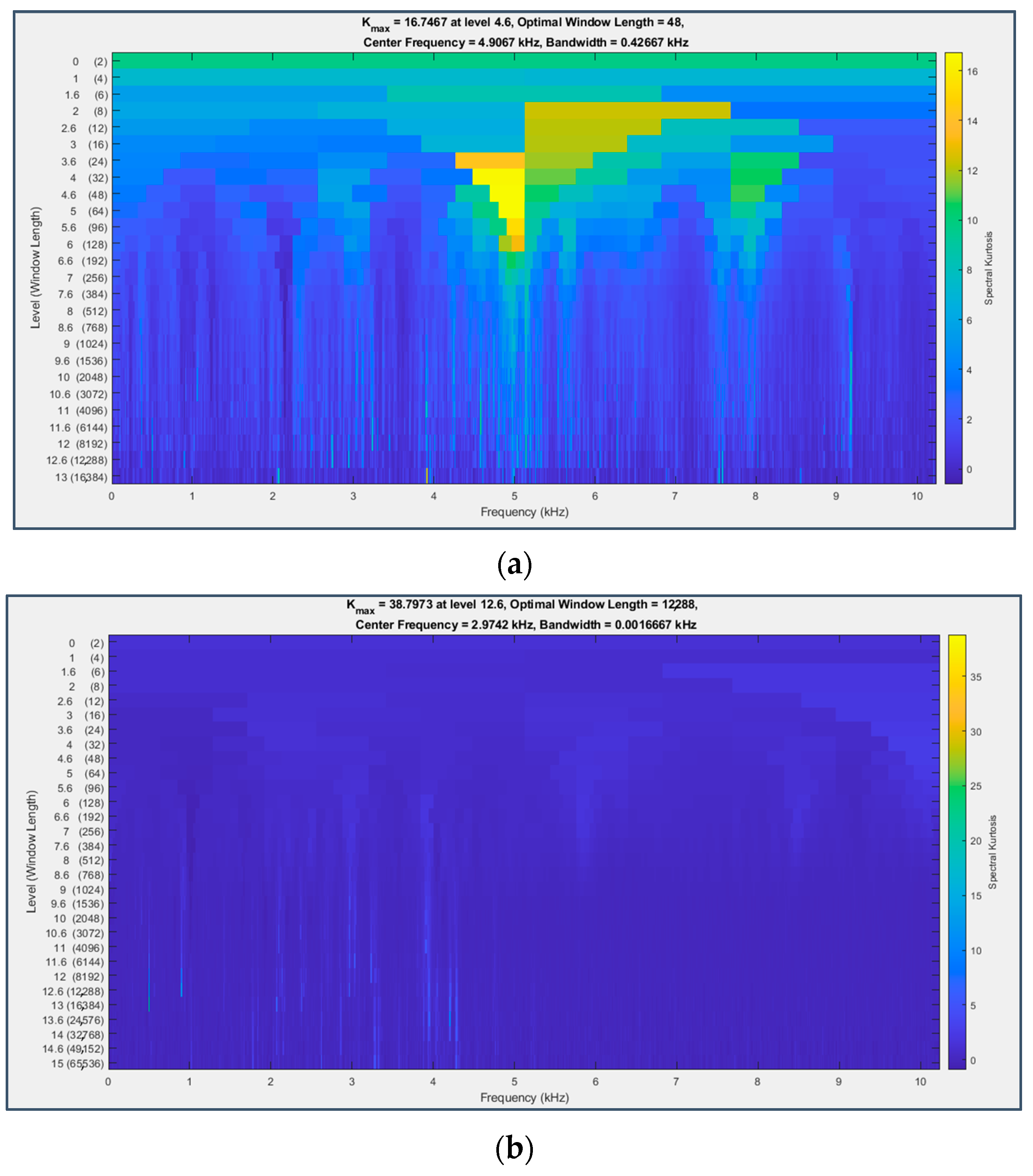
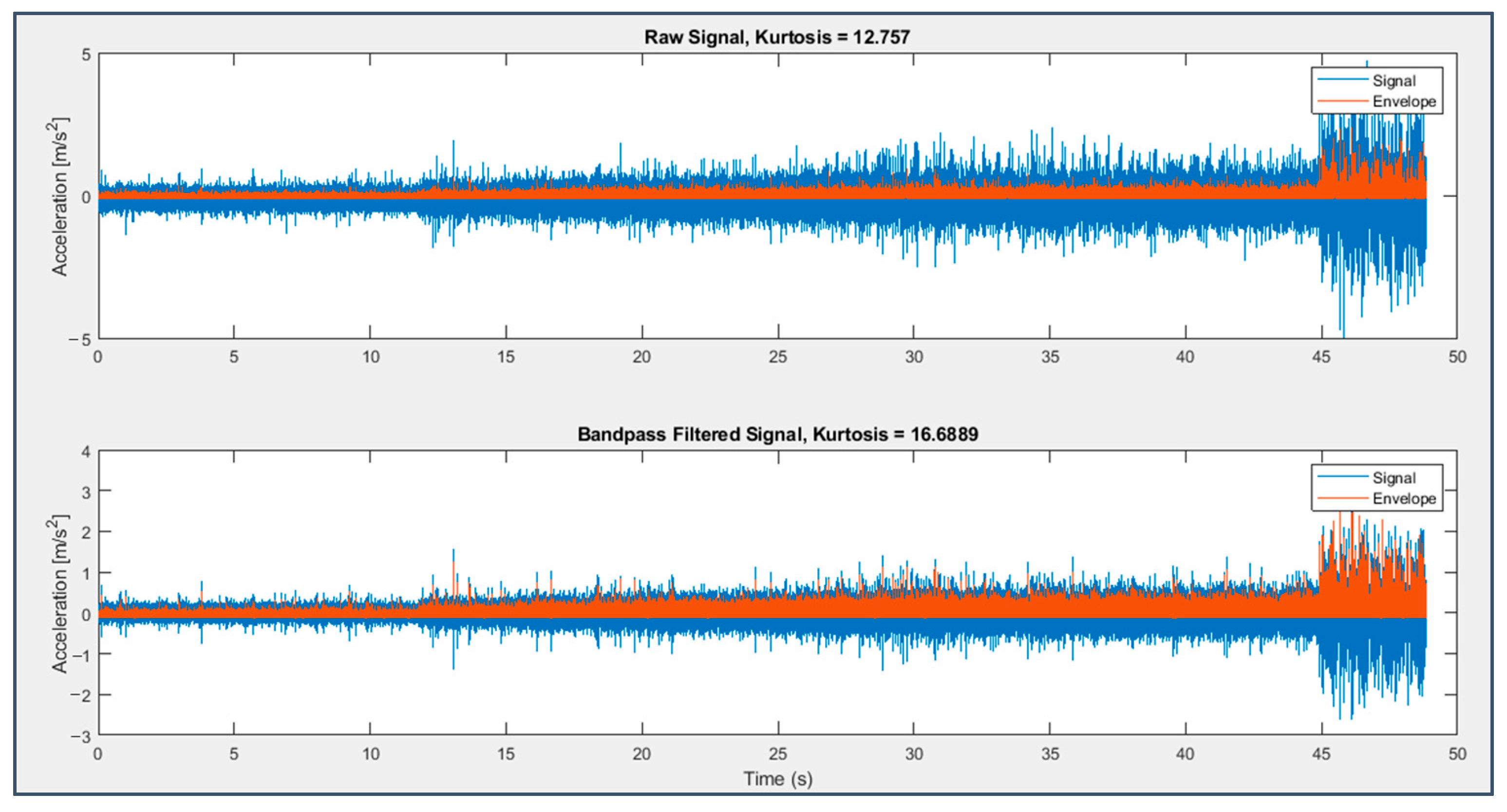
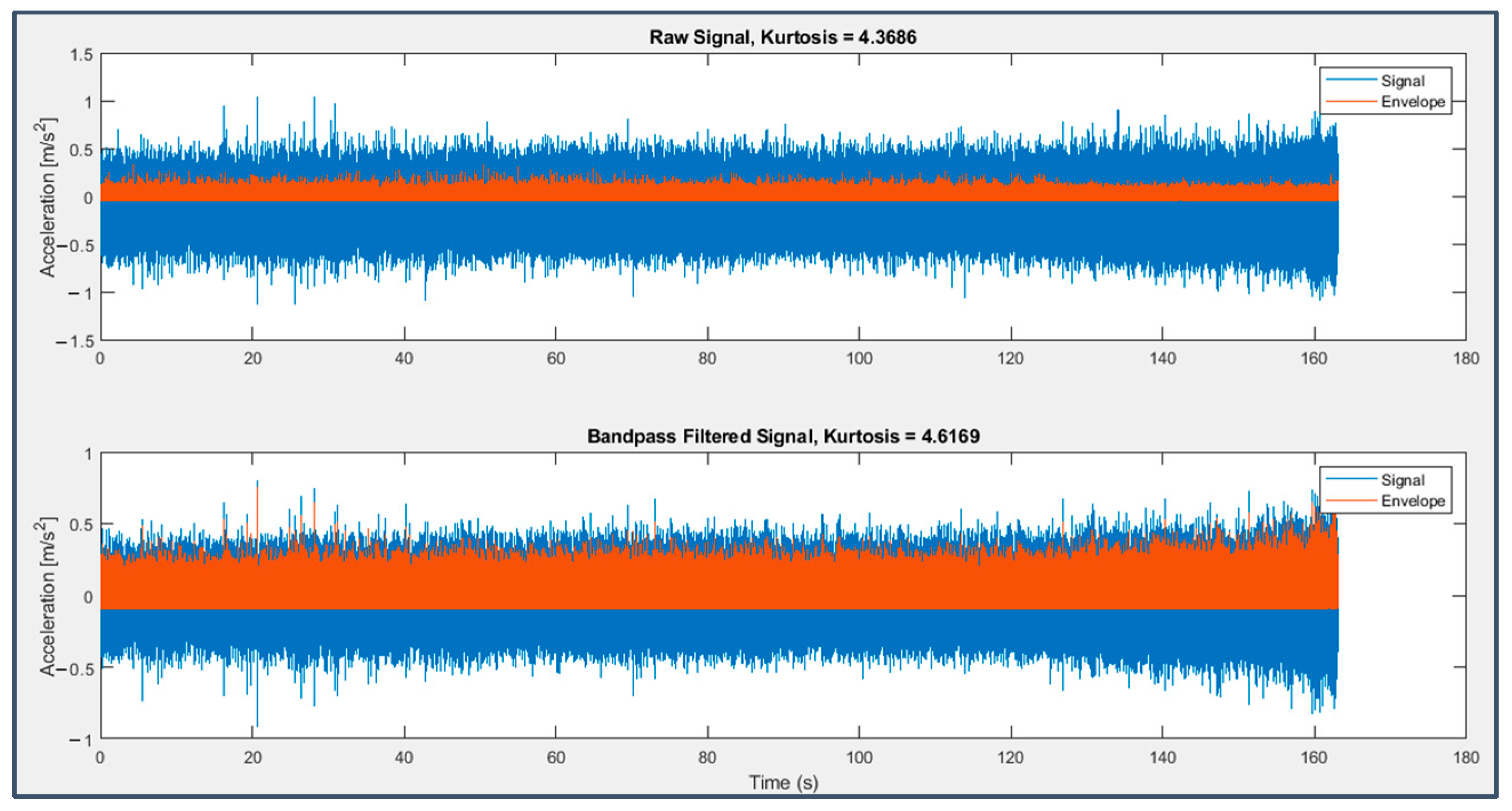
3.2.7. Kurtogram and Filters

With the intention of selecting the most impulsive frequency bands, a Kurtogram has been used to identify the center frequency and bandwidth on which to configure the intervention of a filter (Figure 32).

A 10th order band-pass FIR filter has been chosen, which is able to slightly increase the signal Kurtosis (Figure 33 and Figure 34; nevertheless, after the computation of the SES technique (Figure 35 and Figure 36), it appears clear that the filter brought out a frequency band in which the fault components were not predominant, probably because the impulsiveness detected by the Kurtogram was related to phenomena different from the impacts caused by faults on the surfaces or was ascribable to the signal transmission path.

The use of an adaptive filter applied in the very same way is not beneficial either.

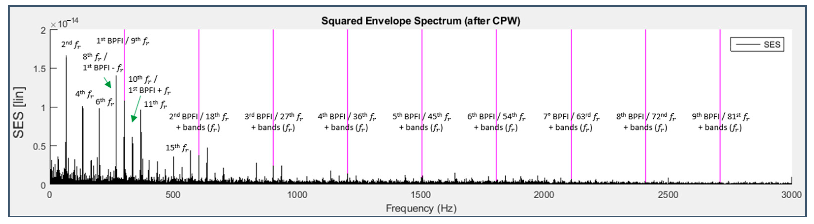
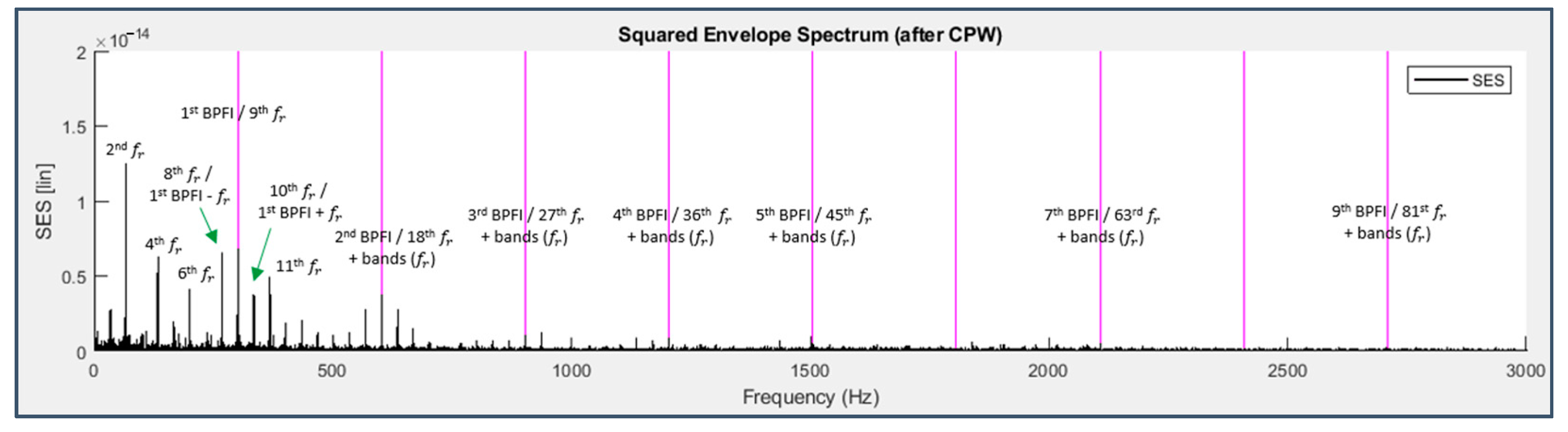
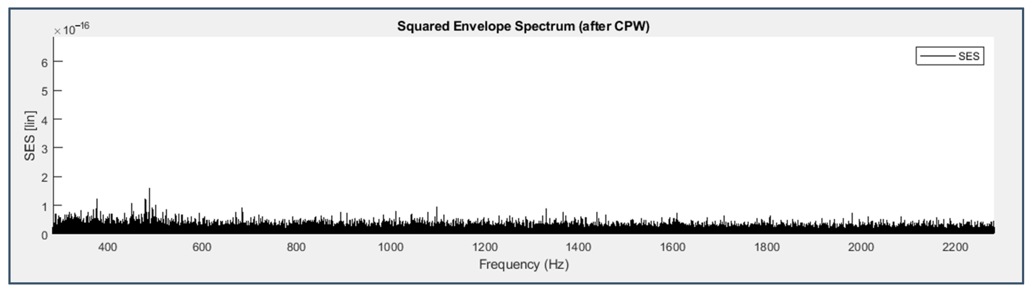
3.2.8. Cepstrum Pre-Whitening (CPW)

Unlike the mostly unsuccessful trials just reported, the use of the Cepstrum Pre-Whitening proves to be a powerful resource for the application under examination; it is a relatively new technique that has gained appreciation both in the literature [39] and in industrial practice [40], but it is not yet included in the most traditional and ever-invoked set of diagnostics techniques. It can be employed in two ways: the first one exploits the real cepstrum to perform the “editing”, removing through liftering the peaks of the periodic components that correspond to impulses at particular harmonics; the second method, far more radical, sets the whole real cepstrum to zero except for the amplitude at the null quefrency, removing both resonances and discrete frequencies, and then resumes to time-domain after a recombination with the unwrapped phase of the original signal, neglected in the real cepstrum. This latter approach is actually easily implemented by dividing the signal Fourier transform by its absolute value and after inverse transforming it back to the time-domain:

$$x_{CPW}\left(t\right)=F^{-1}\left\{\frac{F\left(x\left(t\right)\right)}{\left|F\left(x\left(t\right)\right)\right|}\right\}$$

(24)

The conceptual and operative simplicity of this technique and its limited computational request are as appreciable as the results it provides. The only drawback is represented by the reduction of various orders of magnitude of all the amplitudes, even those that are useful; however, this aspect does not affect its efficacy since the desired components clearly stand out from the others and from noise, which are both significantly mitigated.

Envelope spectra are indeed dominated by the frequency lines of the fault harmonic series: as for bearing 3, Figure 37 and Figure 38 confirm the previously stated conclusion that the inner race fault harmonics are not visible directly but indirectly, through the excitation of those of the shaft rotation frequency that are near to them and of its even ones in general thanks to modulation effects; in the spectrum of bearing 4 (Figure 39, the cage frequency harmonics are undoubtedly present, as well as those of the BPFO, until the 11th one, and those of the BSF are present to a lesser extent (until the 6th one, barely visible), accompanied by the modulation sidebands at a distance equal to the FTF; it is important to note that the strong presence of the harmonics of the shaft and cage rotation frequencies should not be considered a masking factor to be removed—on the contrary, it is just related to faults and ought to be seen as their indirect sign, not present at the beginning of the experiment (Figure 40).

CPW has therefore been capable of deleting all the components unrelated to faults, including the harmonic series based on the fundamental frequencies at 160 Hz and 505 Hz and the peaks at very high frequency coming from structural resonances, leaving the three fault signatures thoroughly visible and unmistakably detectable.

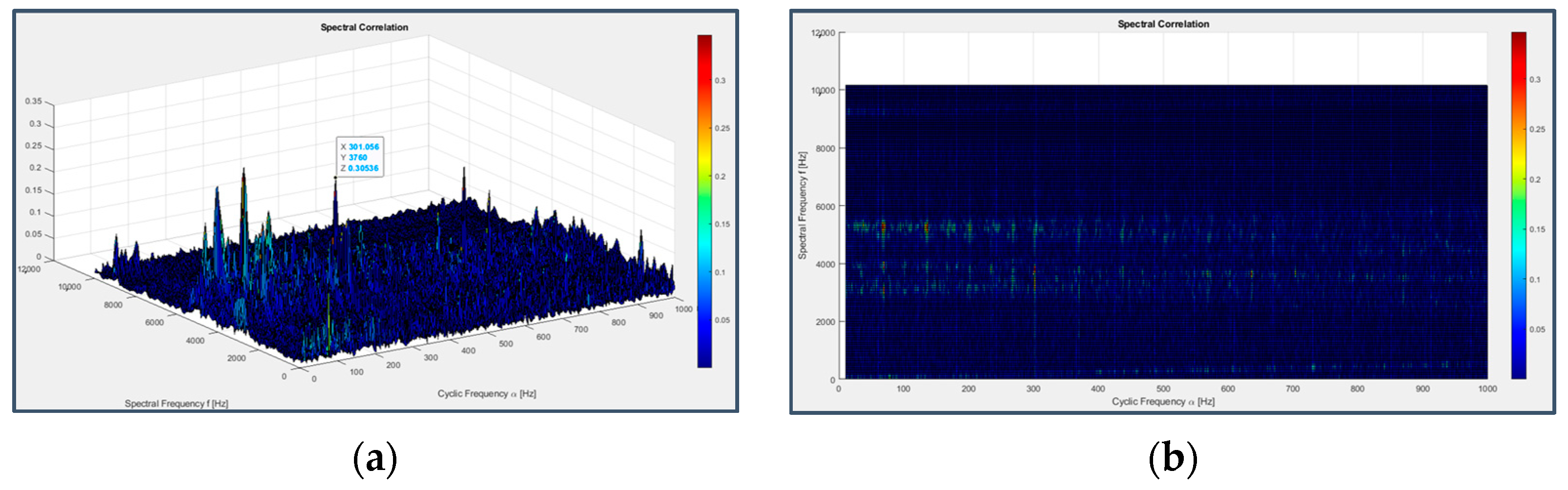
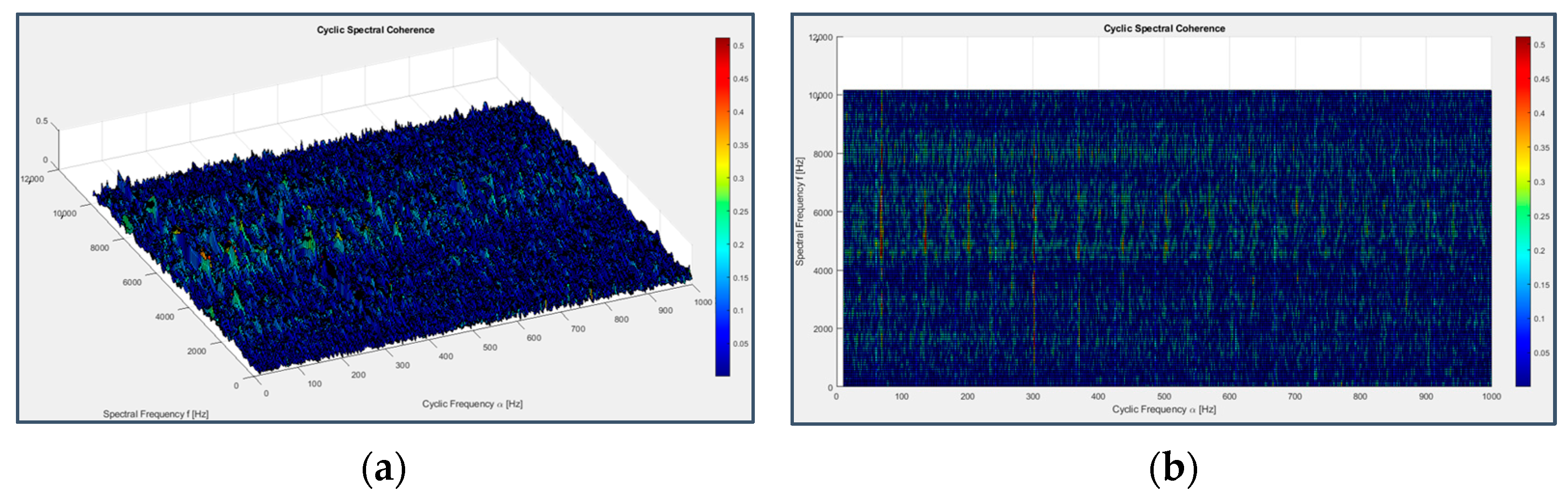
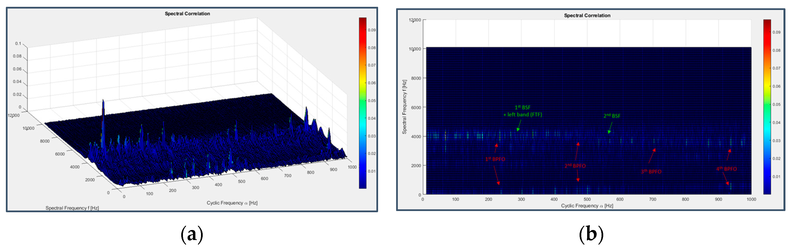
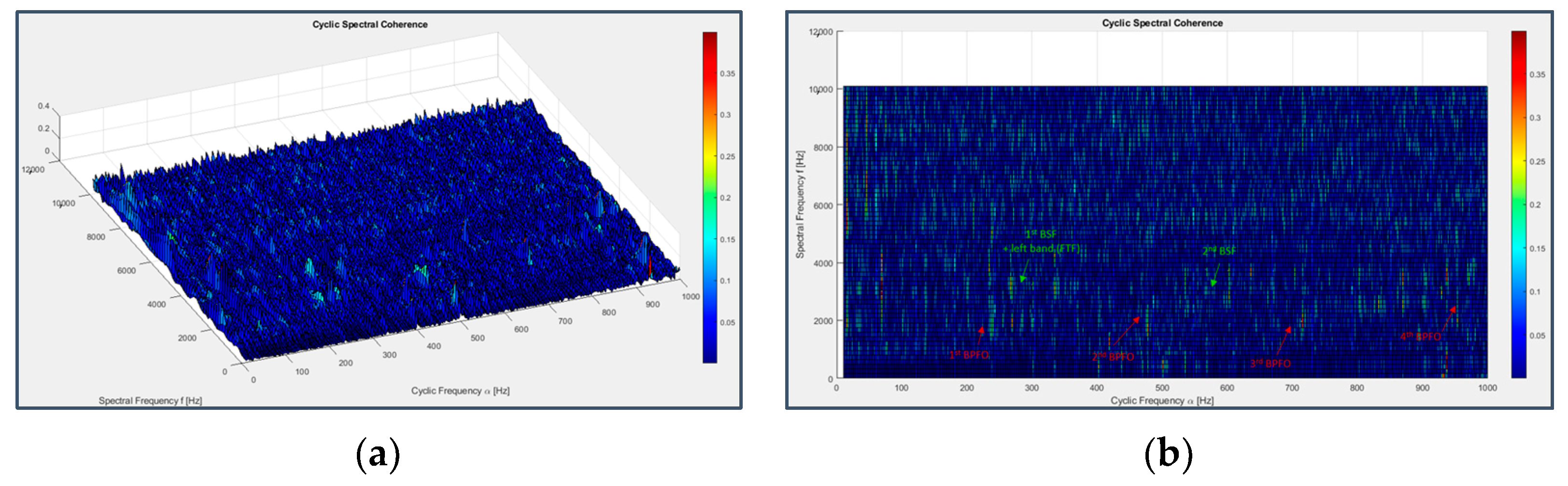
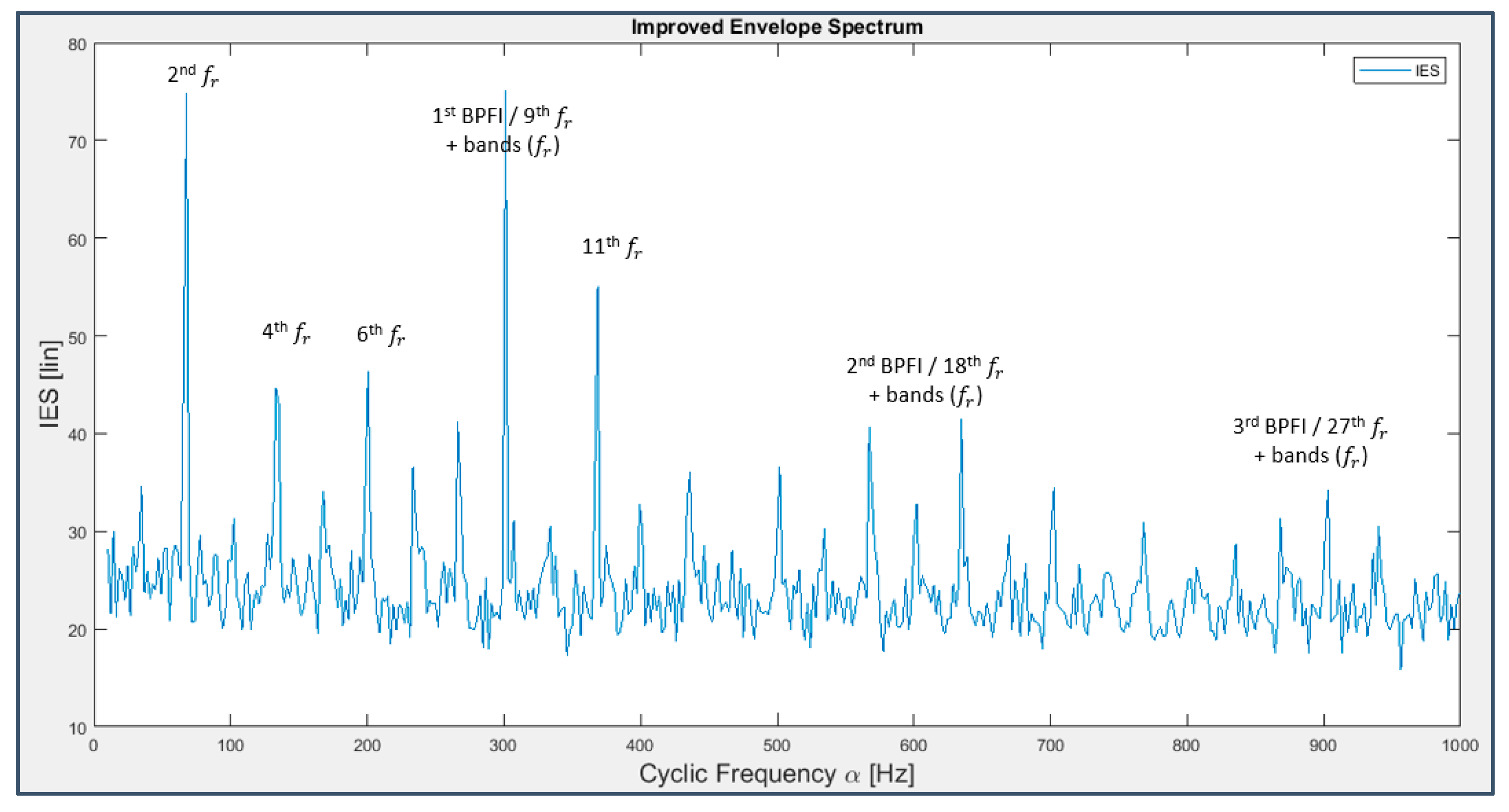
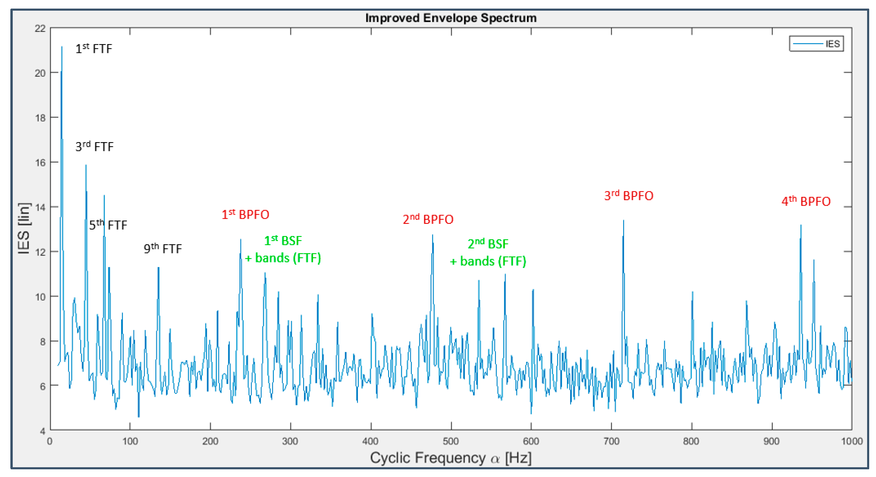
3.2.9. Cyclostationary Analysis

Given that the analysis conducted so far has allowed us to perform the second phase of condition monitoring, namely the fault diagnosis, without taking into consideration the particular nature of the signal in question, for the sake of completeness it is worth trying to apply some techniques specifically formulated for the study of second-order cyclostationary signals, which are the ones actually produced by the damaged bearings. The purpose is twofold: (i) validating the previous conclusions by taking a substantially different point of view, and (ii) testing the efficacy of these tools, which are potentially more powerful but also more complex to understand, interpret and handle.

It is well known that there is a point of connection between stationary and cyclostationary techniques, owing to the mathematical identity between the integral of the Spectral Correlation function made along all the spectral frequencies and the Squared Envelope Spectrum. It seems then reasonable to compute the Improved Envelope Spectrum (IES) in order to verify that it offers information similar to that obtained with the SES and to understand the differences between them, if any.

Three-dimensional chromatic maps displaying Spectral Correlation and Cyclic Spectral Coherence cannot be figured out immediately due to the abundance of information, but seen from above, i.e., projected on the frequency plane, they show a preferential arrangement of the peaks at cyclic frequencies $\alpha$, which correspond to those of faults and their modulating ones (even the harmonics of the shaft rotation frequency and odd harmonics near to those of the BPFI for bearing 3 in Figure 41 and Figure 42 and harmonics of the BPFO, FTF and BSF for bearing 4 in Figure 43 and Figure 44) and at spectral frequencies $f$, which are always exact multiples of 160 Hz or 80 Hz (320 Hz, 3120 Hz, 3760 Hz, 3680 Hz, 3840 Hz, 5280 Hz); these last frequencies were already observed as being related to system periodicities, although it is not possible to surely state their physical origin with the information provided on the dataset.

Coming back to the dependence from a single variable, the IES (Figure 45 and Figure 46), computed as the integral of the Cyclic Spectral Coherence on the spectral frequency band [0 10,000 Hz] (nearly more like an EES than an IES), puts the stress on the same spectral frequencies that represent fault signatures, even if with a bit less emphasis with respect to Figure 37, Figure 38 and Figure 40. This makes a lot of sense because the IES was applied on the raw signal while, in the previous paragraph, the signal was pre-processed via the radical technique of the CPW.

Applying the previous cyclostationary techniques to excerpts of the original signal all along the experiment time duration (omitting the resulting plots for brevity), the fault history can be traced more precisely than it has been before: the inner race fault on bearing 3 occurs almost at the end of the test (33rd–34th day), while the outer race fault on bearing 4 can be detected from day 28 and that on the rolling element is still present from around the 26th day and dominates the other, but it is already less visible in Figure 46, probably due to the progressive smoothing of the fault pit caused by friction.

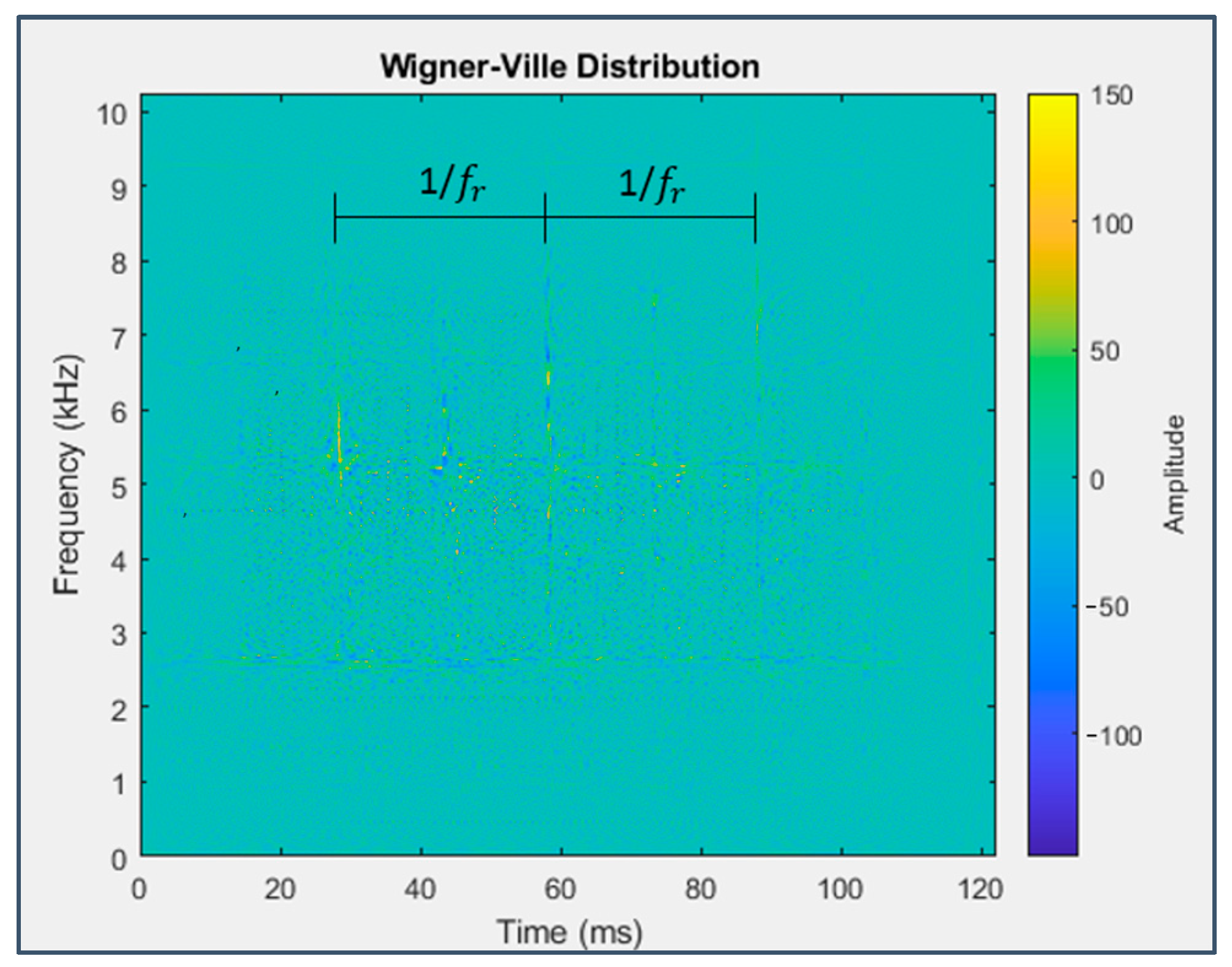
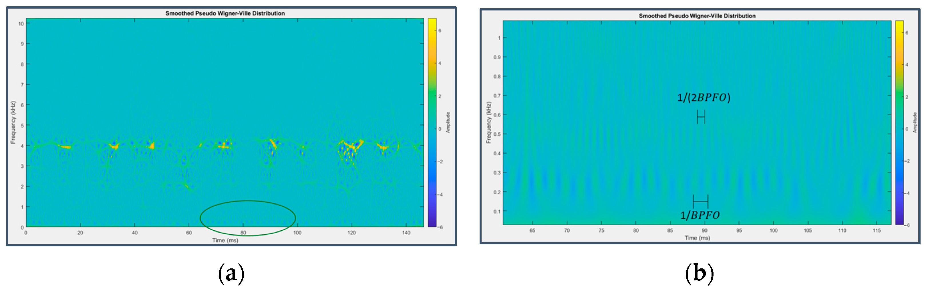
3.2.10. Wigner–Ville Distribution (WVD)

Strictly speaking, WVD has to be ranked among the time-frequency domain techniques, even if it is characterized by a mathematical formulation that is rather similar to that of the cyclostationary techniques and is suitable for the analysis of the same type of signals.

Looking at the respective plots, the presence of cyclic phenomena related to fault development, totally absent in the initial phase, can be detected, albeit more vaguely than before. Figure 47 shows a series of peaks at the spectral frequency of 5280 Hz (still an exact multiple of 160 Hz), spaced from each other by a period (cycle) equal to 30 ms, i.e., the inverse of the shaft rotation frequency f_r. A marked impulsiveness features in Figure 48a at the spectral frequency of 4000 Hz (25 × 160 Hz), and its zoom (Figure 48b) is dominated by a train of alternated chromatic bands at the spectral frequencies of 240 Hz (1.5 × 160 Hz) and 480 Hz (3 × 160 Hz), spaced apart by a time interval equal to the inverse of the BPFO and its double, respectively (about 4 ms and 2 ms).

3.2.11. Comparisons

In this part, in order to recapitulate the obtained results, a list of the 10 fault diagnosis methods previously introduced is reported, where the advantages and disadvantages of each method are described.

• STFT. Advantages: able to detect the higher-order harmonics of the BPFI for bearing 3 and of the BPFO and BSF for bearing 4. Disadvantages: not able to detect the corresponding first-order harmonics.
• PSD. Advantages: able to detect some harmonics of the BPFI for bearing 3 and of the BPFO for bearing 4. Disadvantages: not able to detect the harmonics of the BSF for bearing 4, and presence of frequency lines related to structural resonances.
• SES. Advantages: able to detect the harmonics of the shaft rotation frequency and BPFI for bearing 3 and of the BPFO and BSF for bearing 4. Disadvantages: presence of high noise and masking components.
• TSA + SES. Advantages and disadvantages: exactly the same of SES alone.
• ALP + SES. Advantages and disadvantages: the same of SES alone, with a reduction in part of the background noise.
• Daubechies’ Wavelets + SES. Advantages and disadvantages: the same of SES alone, with a little reduction in noise and masking components.
• FIR filter + SES. Advantages and disadvantages: exactly the same of SES alone.
• CPW + SES. Advantages: able to detect the harmonics of the shaft rotation frequency and BPFI for bearing 3 and of the BPFO and BSF for bearing 4 with very low noise. Disadvantages: reduced amplitude of the response peaks.
• IES. Advantages: able to detect the harmonics of the shaft rotation frequency and BPFI for bearing 3 and of the BPFO and BSF for bearing 4 with relatively low noise. Disadvantages: analysis performed on the raw (i.e., not pre-processed) signal.
• WVD. Advantages: able to detect some harmonics of the shaft rotation frequency for bearing 3 and of the BPFO for bearing 4. Disadvantages: not able to detect the harmonics of the BPFI for bearing 3 and of the BSF for bearing 4.

3.2.12. Diagnostic Accuracy

In this section, the accuracy of the fault diagnosis techniques previously considered is evaluated quantitatively. To this end, we selected the statistical parameter Kurtosis as the diagnostic accuracy index of the specific signal processing technique adopted, which usually denotes the impulsivity of the vibration signal in the time domain. In the present case, Kurtosis is computed in the frequency domain, indicating the impulsivity of the harmonics of the shaft rotation and fault frequencies, i.e., the emerging of the related peaks with respect to noise, and therefore the accuracy of the signal processing method considered.

In

Table 5. Kurtosis of the fault diagnosis techniques considered.

Technique	Bearing	Kurtosis
PSD	3	46.3 (Figure 20)
	4	41.1 (Figure 22)
SES	3	22.7 (Figure 24)
	4	17.5 (Figure 25)
TSA + SES	3	23.0 (Figure 26)
	4	17.8 (Figure 27)
ALP + SES	3	24.2 (Figure 28)
	4	18.2 (Figure 29)
Wavelets + SES	3	22.9 (Figure 30)
	4	17.5 (Figure 31)
FIR Filter + SES	3	51.2 (Figure 34)
	4	38.6 (Figure 36)
CPW + SES	3	86.0 (Figure 38)
	4	81.7 (Figure 40)
IES	3	65.7 (Figure 45)
	4	58.6 (Figure 46)

, the values of Kurtosis computed for the different fault diagnosis techniques previously considered are reported. Signals from both sensor 6 on bearing 3 (last 49 s) and sensor 7 on bearing 4 (last 163 s) are processed within the frequency bandwidth 0–1000 Hz.

These analyses make it explicit that all the employed techniques have produced rather impulsive trends. While PSD shows higher values of Kurtosis than SES, all the combinations of the latter with other preliminary methods lead to a trivial increase in the numbers in the third column. Indeed, the maximum values of Kurtosis are found for the combination of CPW and SES, and for IES methods, and therefore it is confirmed that these techniques are the most effective in the fault diagnosis of the IMS first bearing dataset. It must be stressed that the FIR Filter also exhibits significant values but detects dynamics not directly related to the phenomenon of faults, as mentioned above.

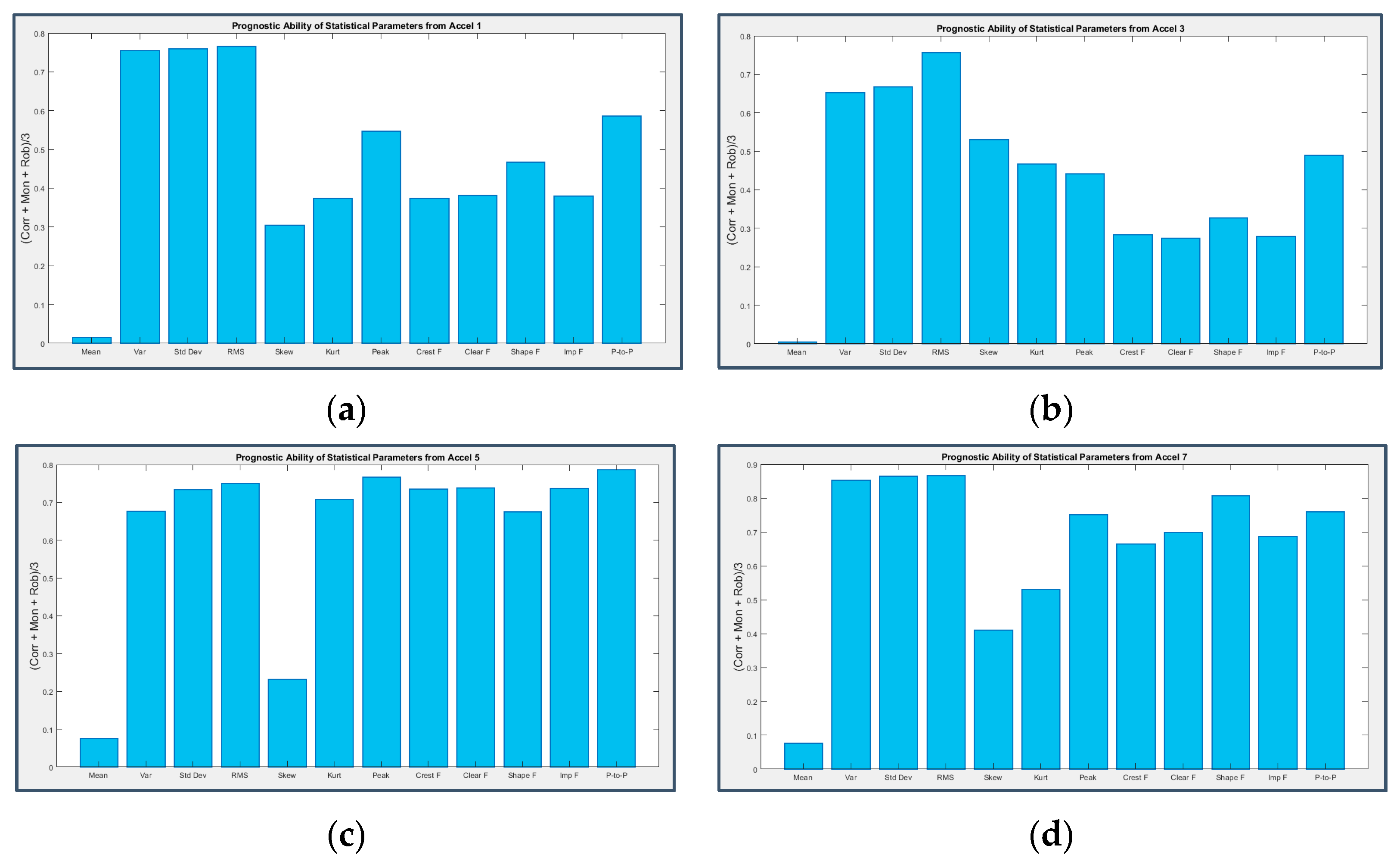
3.3. Fault Prognosis

After fault detection and diagnosis, the third phase required to accomplish the whole condition monitoring of a signal is the fault prognosis, which implies making a prediction about the future signal trends, beyond the end of real data, with a certain level of probabilistic confidence, with the goal of estimating the component’s Remaining Useful Life (RUL). This operation represents the key point to identify the optimal time to replace a mechanical part, in the trade-off between the cost minimization due to the intervention on the system and the cost of the new component, fully exploiting the service life of the one to remove on one hand, and the major cost to bear in case of a catastrophic failure occurs on the other, leading to a harmful stop of production, which is absolutely to be prevented.

Prognosis issues are often carried out making use of advanced data-driven techniques belonging to the domain of AI and specifically of Machine Learning, which are programmatically beyond the scope and the intention of this paper. This section is meant for providing a first glance at that field, identifying the most recommended statistical parameters for prognostic considerations on the IMS dataset.

As stated before, the bearings’ end of life were conventionally determined through a lubricant-based analysis; however, it is still feasible to determine how reliable information extrapolated with statistical operators may be about the behavior of the damaged components if brought to the extreme of degradation.

For this reason, the previously mentioned parameters of Correlation, Monotonicity and Robustness, typical indicators used in health management, have been computed on the statistical tools, similarly to what was conducted in [20], at first on every second of acquisition, then averaging the results on the entire test duration and finally obtaining a single quantity for each statistical parameter and each bearing as the average of the three indexes, in the same way adopted for Hjorth’s parameters and Detectivity.

Histograms depicted in Figure 49 clearly suggest that Mean and Skewness are not proper instruments for prognostic operations, as they were not so useful for fault detection either, while RMS value, Variance, Standard Deviation and Peak-to-Peak prove to be the most reliable quantities to be used as a solid base for future estimations. It is interesting to notice that, as may be expected, the parameters evaluated on the signals coming from the two damaged bearings perform better as prognostic tools than when applied on the healthy components.

4. Discussion

From the analyses previously conducted, the following considerations can be drawn on the efficacy of the involved diagnostic techniques for the study of IMS dataset 1:

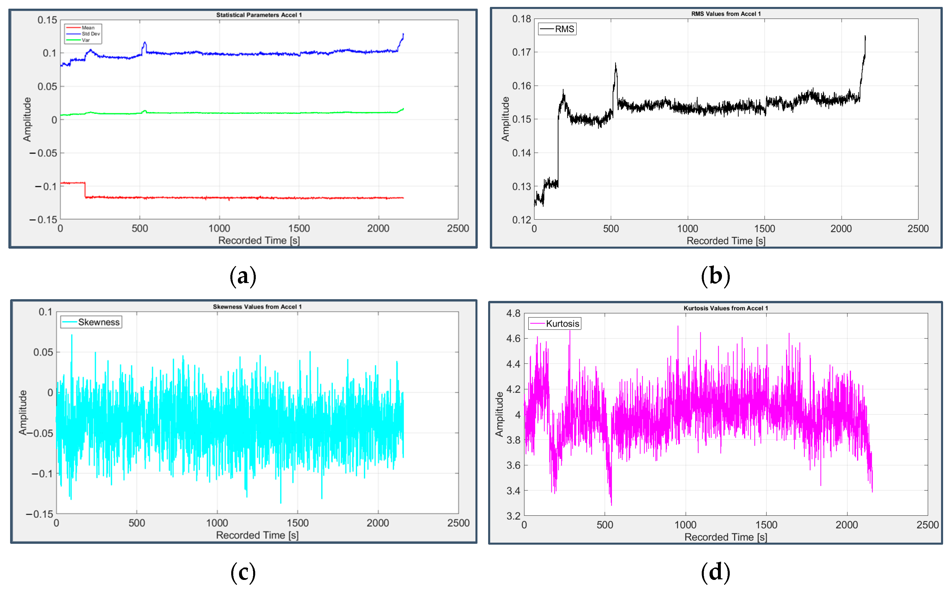
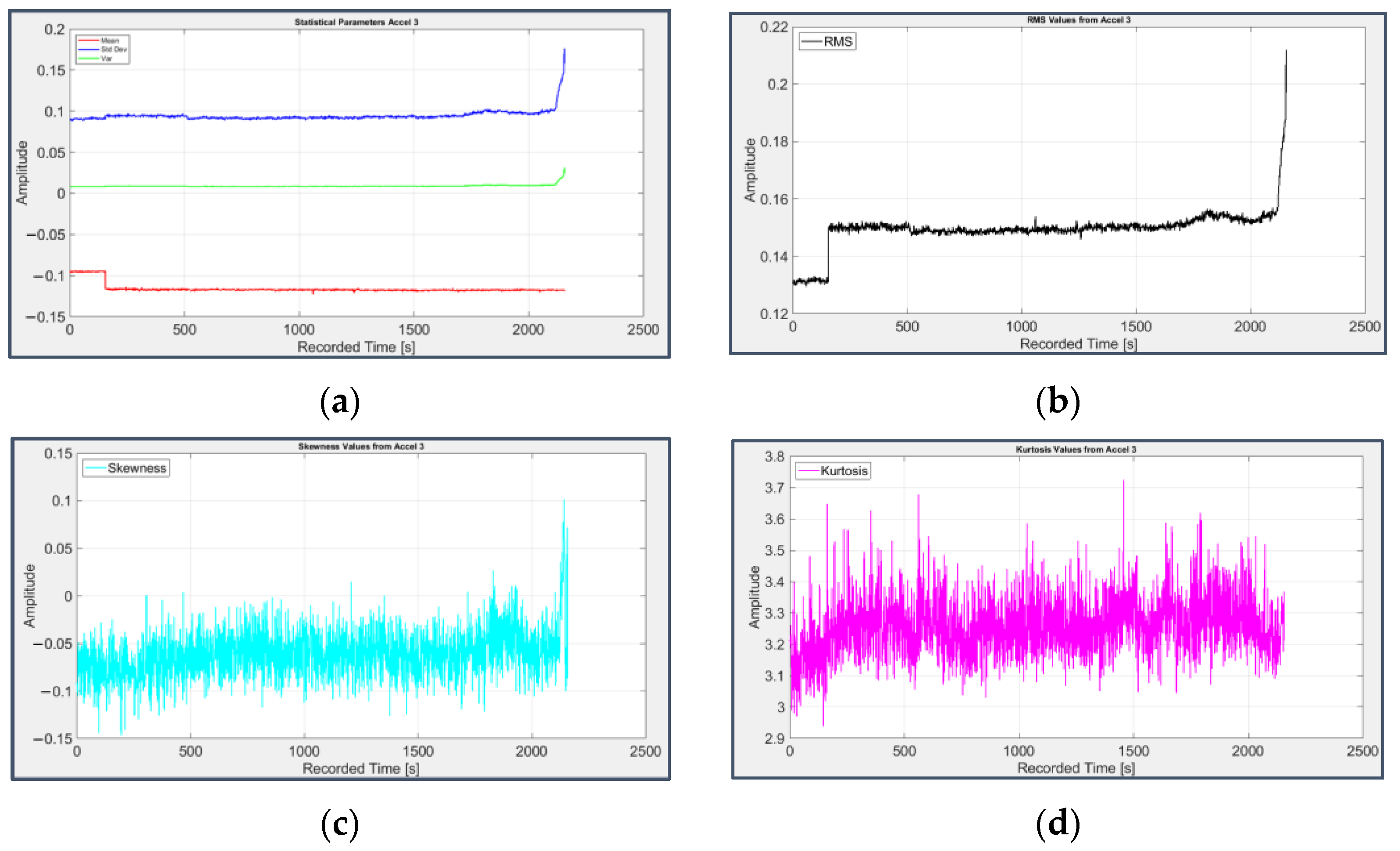
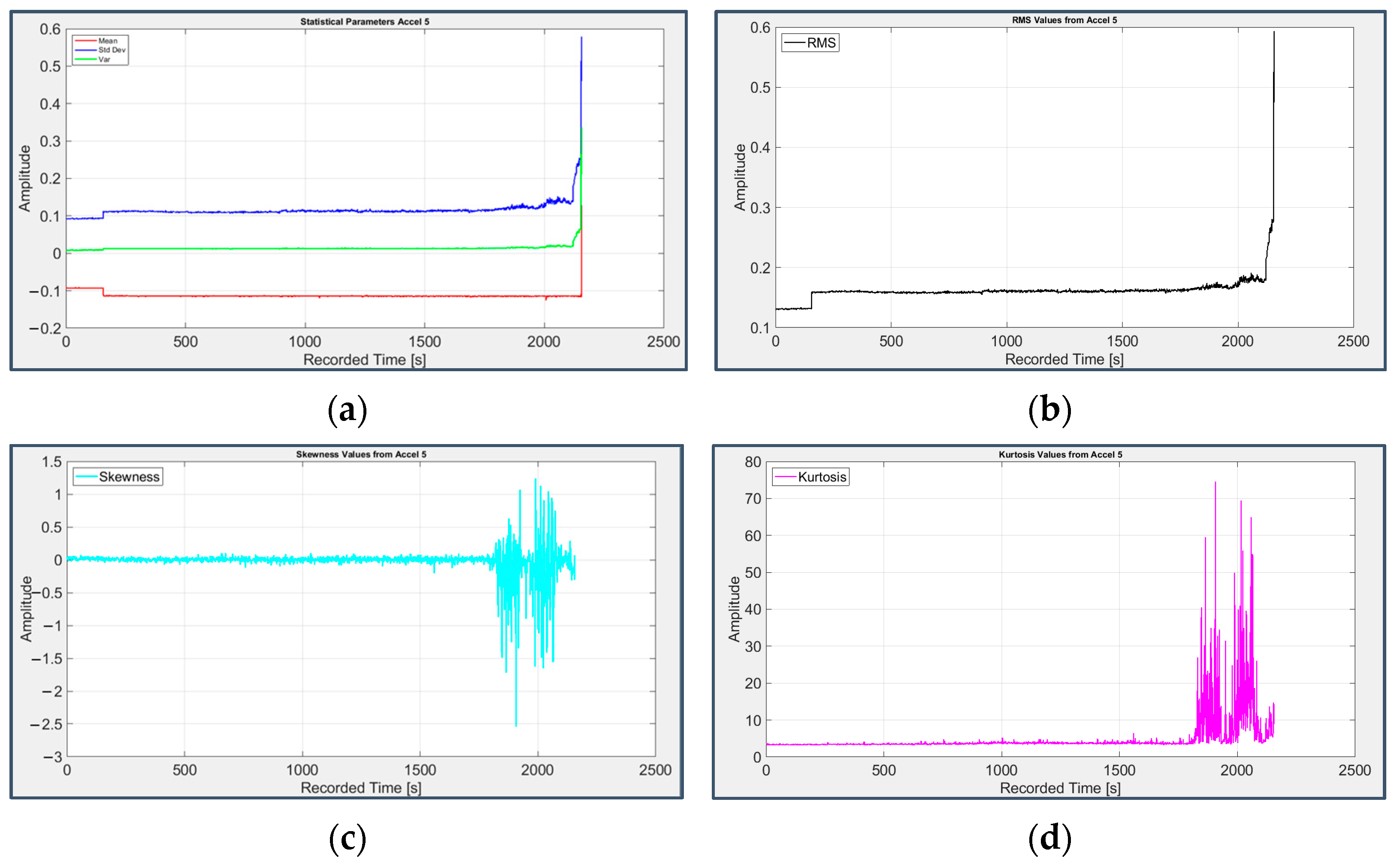
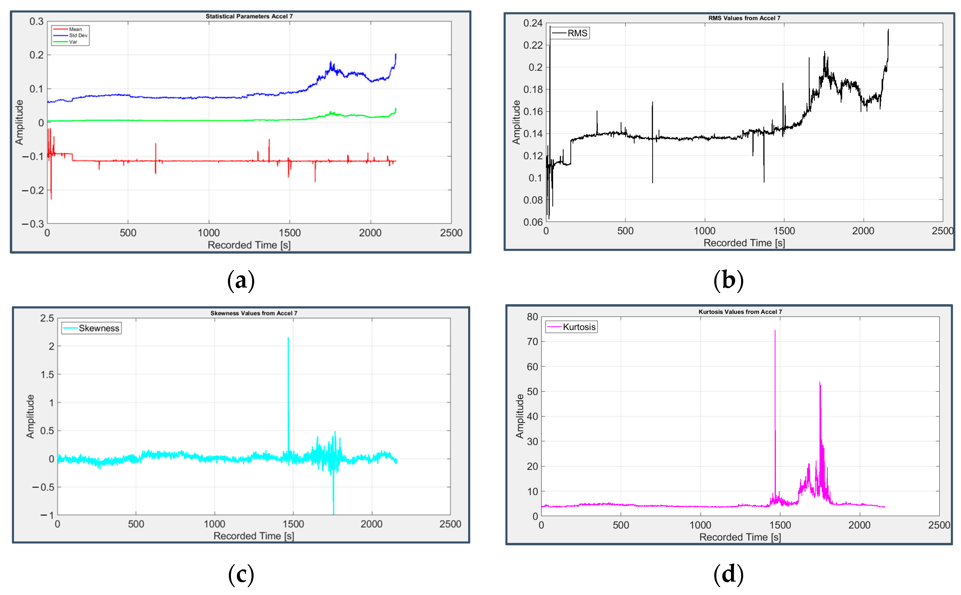
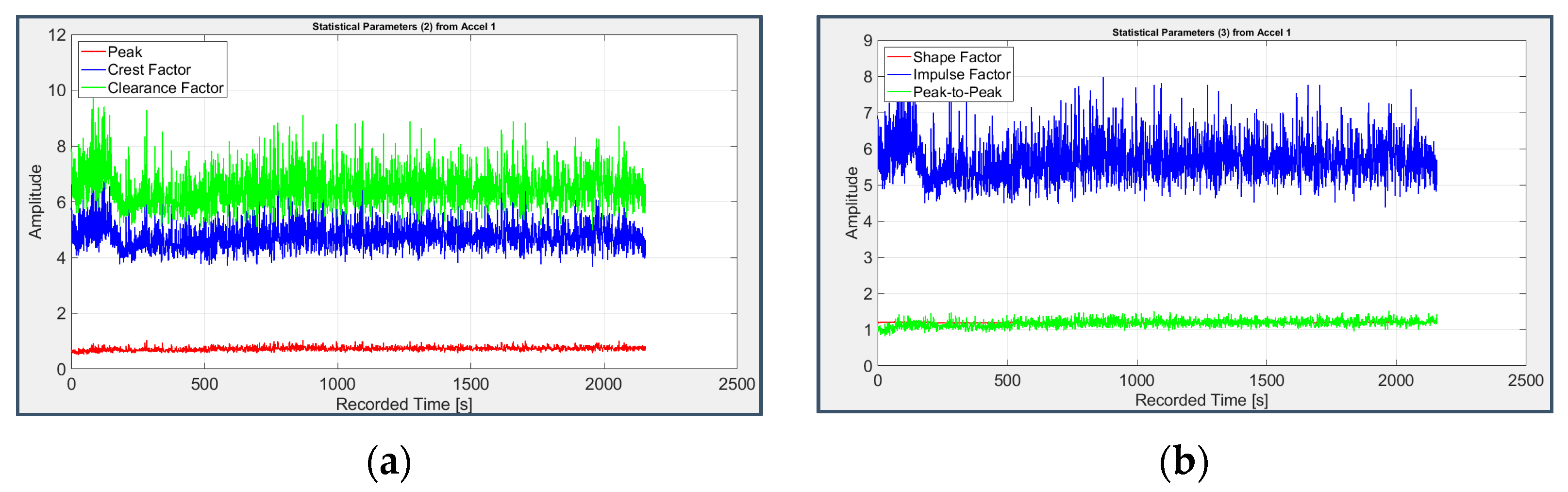
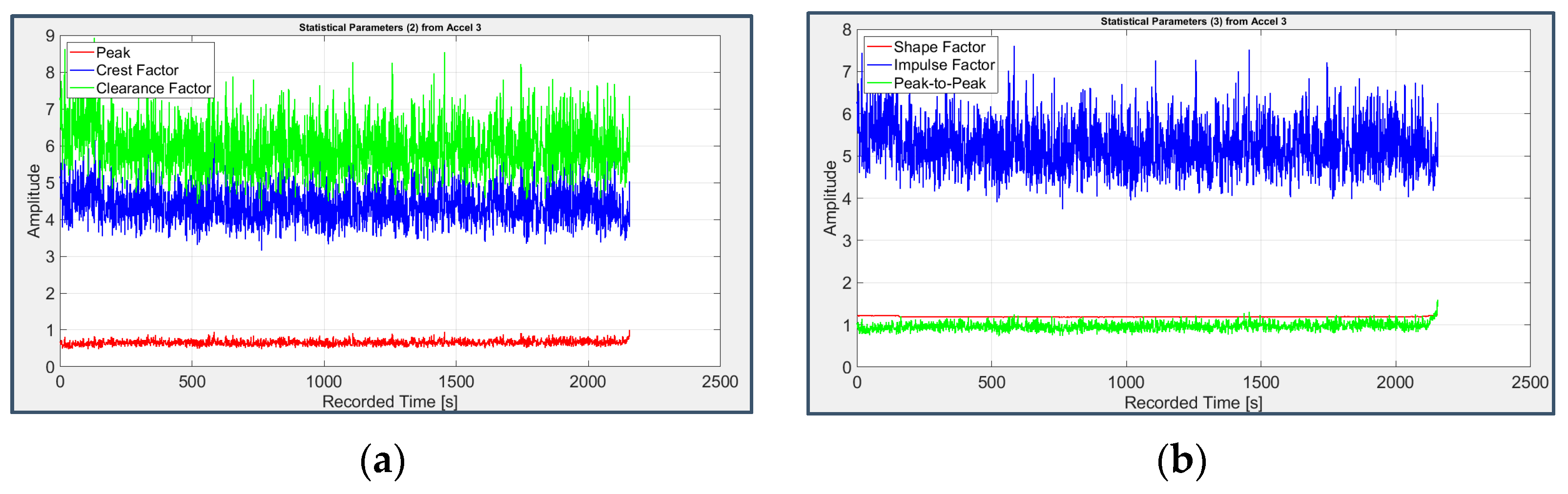
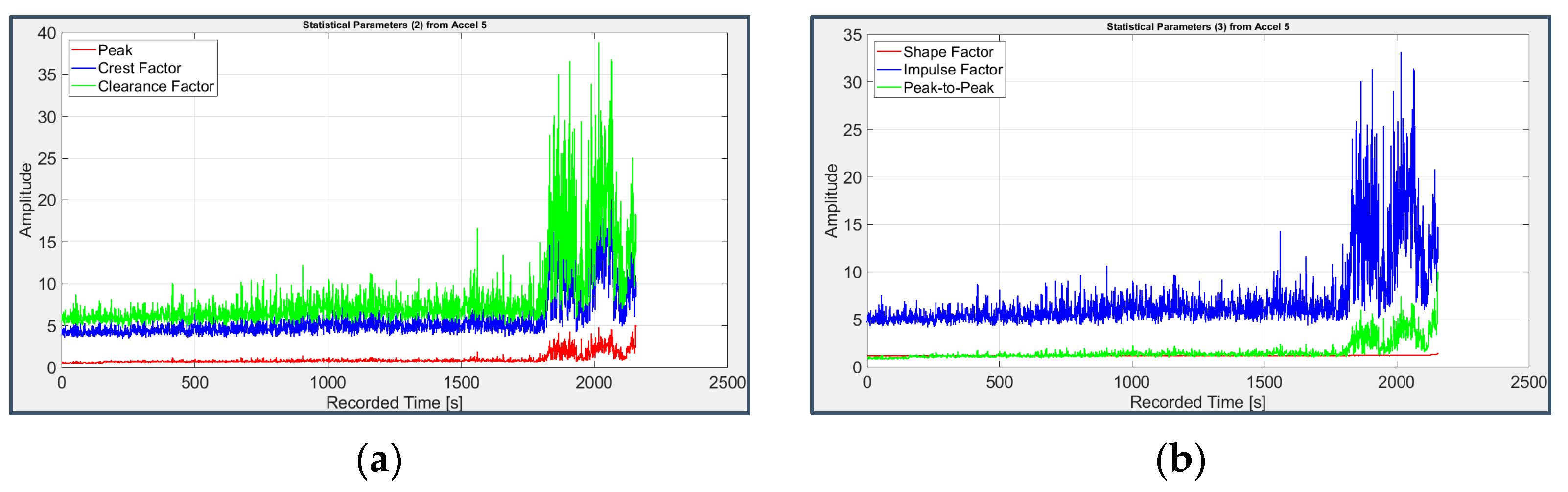
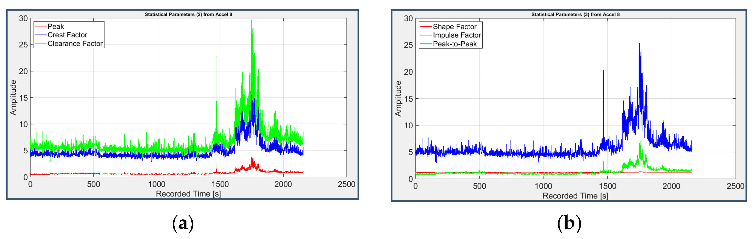
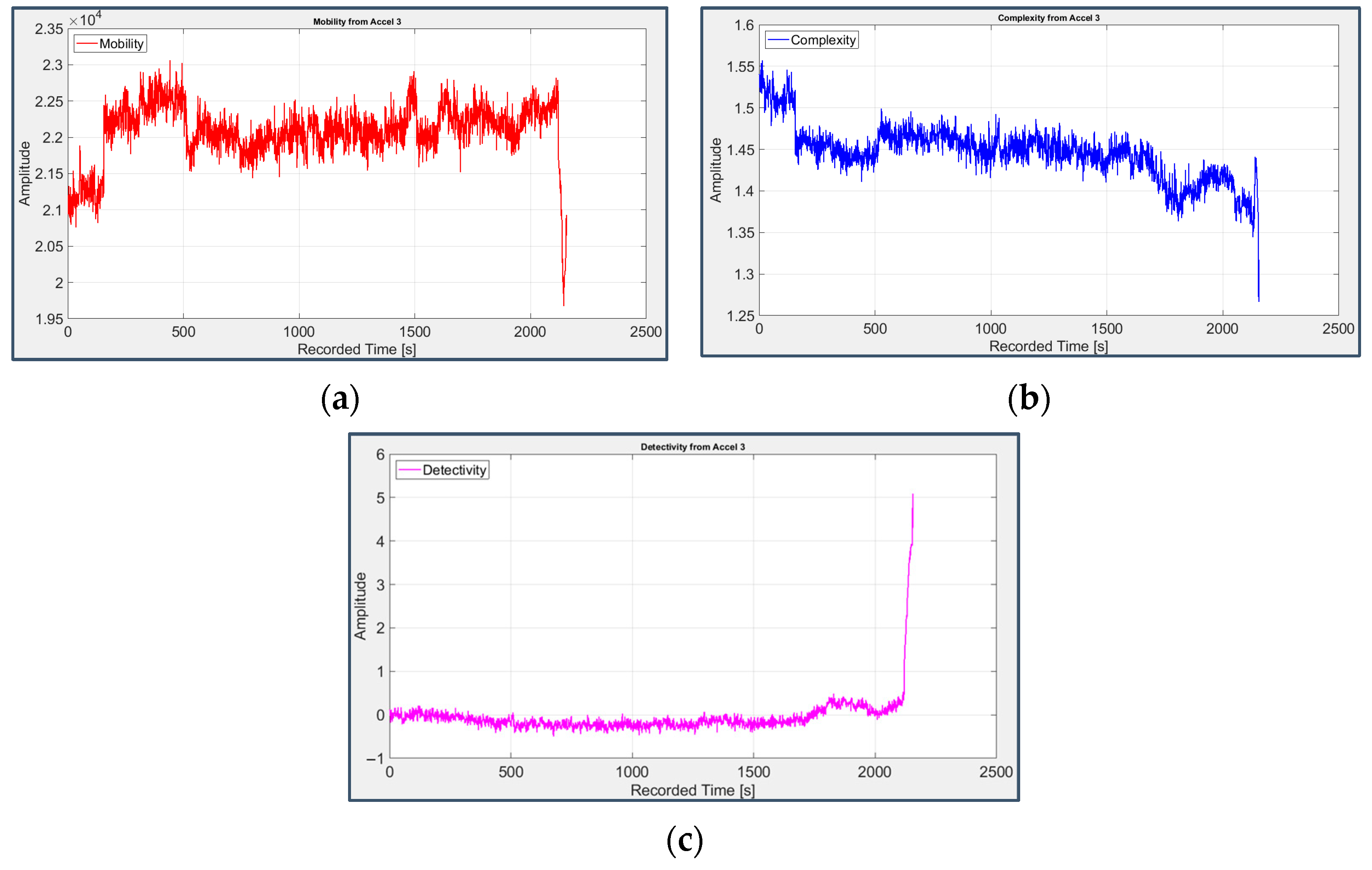
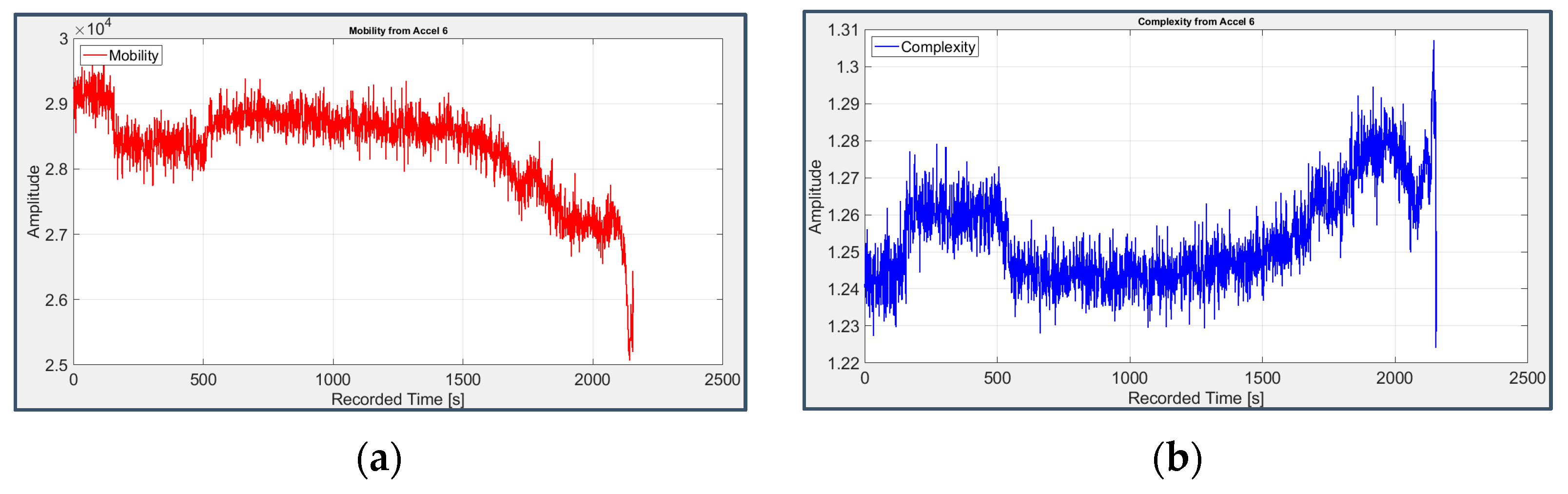
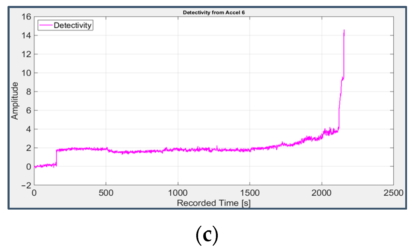
• The initial statistical approach allowed the fault detection phase to be executed, bringing to light the occurrence of different faults on bearings 3 and 4, and suggesting the time excerpts of the signal to focus on in the following analyses: in particular, RMS value, Kurtosis and Detectivity were proven to be the most informative statistical parameters.
• Diagnostic techniques, such as STFT, PSD and SES, even individually, provided a fundamental contribution to identifying the exact nature and temporal location of faults throughout the experiment, also taking advantage of the comparison with faultless signals, at the beginning of the test or coming from healthy bearings; it was then possible to confirm the diagnostic report diffused by the IMS Center itself, which attests the presence of:

  -

  A rather late inner race fault on bearing 3, occurring since day 32, which does not show directly but through the excitation of the spectral harmonics of the shaft rotation frequency; the latter also has modulation effects on the BPFI (even though the interpretation of this fault as located at multiple frequencies of 301 Hz instead of the nominal 297 Hz is still potentially acceptable);

  -

  An outer race fault on bearing 4, detectable for certain from day 28, due to the emergence of various harmonics of the BPFO, without modulating phenomena;

  -

  A rolling element fault on bearing 4, detectable from day 26, with the appearance of the harmonics of the BSF and modulated by those of the cage rotation (FTF), raised themselves by the fault.

On the other hand, since these techniques have been applied directly on the raw (i.e., not pre-processed) signal, they then present high noise and masking components within the amplitude–frequency response pattern, and therefore they must be preceded by suitable signal processing methods to obtain accurate results.

• TSA, ALP and Daubechies’ Wavelets did not prove to be sufficiently useful as signal pre-treatment techniques in combination with SES.
• FIR and adaptive filters based on the Kurtogram were not able to select the frequency band dominated by fault signs.
• The CPW technique turned out to be a very powerful and efficient tool to pre-whiten the signal in combination with SES, by removing all the masking components and noise and therefore highlighting the fault signatures.
• The second-order cyclostationary techniques, especially IES, which are directly applied on the raw signal, were able to correctly detect the harmonics of the fault frequencies for the defective bearings presenting relatively low noise levels.
• It should be underlined that CPW and IES, which were found to be the most useful techniques, were used for the first time in the present work for the diagnostics of the IMS rolling bearing dataset.
• The brief insight made into the prognosis domain, to quantify the suitability of statistical parameters to make predictions on the signal future trends, represents an interesting starting point that may be worthy of being further developed.

5. Conclusions

A comparison among several signal processing techniques for the diagnostics of the first rolling bearing dataset released by NASA IMS Center was carried out. It was found that the combination of Cepstrum Pre-Whitening and Squared Envelope Spectrum provides a very efficient diagnostic method. In particular, CPW turned out to be a powerful tool to pre-whiten the signal, removing all masking components and noise, and therefore highlighting the fault signatures within the SES. Moreover, it was found that also the Improved Envelope Spectrum allows the harmonics of the fault frequencies of the defective bearings to be properly identified. The IES, as a second-order cyclostationary technique, is directly applied on the raw signal, thus providing a response from a different point of view, deeply related to the true nature of the signal under test.

In the Authors’ opinion, the successful application of traditional as well as more advanced and non-conventional vibration signal-based condition monitoring techniques to analyze the first of the three datasets made available by NASA IMS Center can be considered as a positive example of the efficacy of these mathematical tools to accomplish the predictive maintenance of rotating machineries.

To conclude, the Authors’ point of view is that, despite the large and recent diffusion of data-driven approaches, which represent promising methods particularly appreciated for fault prognosis, vibration signal-based techniques still remain essential and irreplaceable in light of the deep and detailed information they provide on the actual nature of the signal; therefore, the best way to perform condition monitoring should be the combined use of classical signal-based and new data-driven techniques.

References

1. Randall, R.B. Vibration-Based Condition Monitoring: Industrial, Aerospace and Automotive Applications, 1st ed.; John Wiley & Sons, Ltd.: Chichester, UK, 2011. [Google Scholar]
2. Andhare, A. Condition Monitoring of Rolling Element Bearings: Vibration Analysis and Diagnostics of Tapered Roller Bearings, Using Time and Frequency Domain Methods, 1st ed.; Lambert Academic Publishing: London, UK, 2010. [Google Scholar]
3. Randall, R.B.; Antoni, J. Rolling element bearing diagnostics—A tutorial. Mech. Syst. Signal Process. 2011, 25, 485–520. [Google Scholar] [CrossRef]
4. Tiboni, M.; Remino, C.; Bussola, R.; Amici, C. A Review on Vibration-Based Condition Monitoring of Rotating Machinery. Appl. Sci. 2022, 12, 972. [Google Scholar] [CrossRef]
5. Sawalhi, N.; Ganeriwala, S. Analysis and Signal Processing of a Gearbox Vibration Signal with a Defective Rolling Element Bearing. Appl. Cond. Monit. 2016, 4, 71–85. [Google Scholar]
6. Pennacchi, P.; Chatterton, S.; Vania, A. Diagnostics of Roller Bearings Faults During Long-Lasting Tests. In Advances in Italian Mechanism Science. IFToMM ITALY 2020. Mechanisms and Machine Science; Springer: Cham, Switzerland, 2021; pp. 687–698. [Google Scholar] [CrossRef]
7. Malla, C.; Panigrahi, I. Review of Condition Monitoring of Rolling Element Bearing Using Vibration Analysis and Other Techniques. J. Vib. Eng. Tech. 2018, 7, 407–414. [Google Scholar] [CrossRef]
8. Zhu, K.; Yue, X.; Sun, D.; Xiao, S.; Hu, X. Rolling Bearing Fault Feature Extraction Using Local Maximum Synchro-squeezing Transform and Global Fuzzy Entropy. Int. J. Acoust. Vib. 2022, 27, 37–44. [Google Scholar] [CrossRef]
9. Senapaty, G.; Rao, S. Vibration based condition monitoring of rotating machinery. MATEC Web Conf. 2018, 144, 01021. [Google Scholar] [CrossRef]
10. Golafshan, R.; Jacobs, G.; Berroth, J. Investigation of Rolling Bearing Condition Monitoring Techniques Based on Long Term Run-to-Failure Vibration Data. Bear. J. Vol. 2018, 3, 107–118. [Google Scholar] [CrossRef]
11. Moshrefzadeh, A. Condition monitoring and intelligent diagnosis of rolling element bearings under constant/variable load and speed conditions. Mech. Syst. Signal Process. 2021, 149, 107–153. [Google Scholar] [CrossRef]
12. Borghesani, P.; Shahriar, R. Cyclostationary analysis with logarithmic variance stabilization. Mech. Syst. Signal Process. 2016, 70–71, 51–72. [Google Scholar] [CrossRef]
13. Gousseau, W.; Antoni, J.; Girardin, F.; Griffaton, J. Analysis of the Rolling Element Bearing Data Set of the Center for Intelligent Maintenance Systems of the University of Cincinnati. CM2016; HAL Open Science: Charenton, France, 2016; Available online: https://hal.science/hal-01715193 (accessed on 10 January 2023).
14. Qiu, H.; Lee, J.; Lin, J. Wavelet filter-based weak signature detection method and its application on rolling element bearing prognostics. J. Sound Vib. 2006, 289, 1066–1090. [Google Scholar] [CrossRef]
15. Zhichao, W.; Hong, X.; Shaomin, Z.; Bo, Y.; Binsen, P.; Jiyu, Z.; Yingying, J. Research on fault diagnosis method of rotating machinery based on EWT-Threshold denoising and teager energy spectrum. In Proceedings of the 30th European Safety and Reliability Conference and the 15th Probabilistic Safety Assessment and Management Conference, Venice, Italy, 1–5 November 2020. [Google Scholar]
16. Cavalaglio Camargo Molano, J.; Strozzi, M.; Rubini, R.; Cocconcelli, M. Analysis of NASA bearing dataset of the University of Cincinnati by means of Hjorth’s parameters. In Proceedings of the International Conference on Structural Engineering Dynamics ICEDyn 2019, Viana do Castelo, Portugal, 24–26 June 2019; Available online: https://hdl.handle.net/11380/1203704 (accessed on 10 January 2023).
17. Jiyu, Z.; Hong, X.; Zhichao, W. Research on identification method of bearing performance degradation in NPP Based on GG clustering. In Proceedings of the 30th European Safety and Reliability Conference and the 15th Probabilistic Safety Assessment and Management Conference, Venice, Italy, 1–5 November 2020. [Google Scholar]
18. Mortada, M.-A.; Yacout, S.; Lakis, A. Diagnosis of rotor bearings using logical analysis of data. J. Qual. Maint. Eng. 2011, 17, 371–397. [Google Scholar] [CrossRef]
19. Hosseinpour, F.; Behzad, M.; Zio, E. Model-based prognostic of the remaining useful life of bearings considering model parameter uncertainty. In Proceedings of the 30th European Safety and Reliability Conference and the 15th Probabilistic Safety Assessment and Management Conference, Venice, Italy, 1–5 November 2020. [Google Scholar]
20. Sim, J.; Kim, S.; Park, H.J.; Choi, J.-H. A Tutorial for feature engineering in the prognostics and health management of gears and bearings. Appl. Sci. 2020, 10, 5639. [Google Scholar] [CrossRef]
21. Wang, J.; Wang, D.; Wang, S.; Li, W.; Song, K. Fault Diagnosis of Bearings Based on Multi-Sensor Information Fusion and 2D Convolutional Neural Network. IEEE Access 2021, 9, 23717–23725. [Google Scholar] [CrossRef]
22. Eren, L.; Ince, T.; Kiranyaz, S. A Generic Intelligent Bearing Fault Diagnosis System Using Compact Adaptive 1D CNN Classifier. J. Signal Process. Syst. 2019, 91, 179–189. [Google Scholar] [CrossRef]
23. Tobon-Mejia, D.A.; Medjaher, K.; Zerhouni, N.; Tripot, G. A data-driven failure prognostics method based on mixture of Gaussian hidden Markov models. IEEE Trans. Reliab. 2012, 61, 491–503. [Google Scholar] [CrossRef] [Green Version]
24. Jianbo, Y. Health condition monitoring of machines based on hidden Markov model and contribution analysis. IEEE Trans. Instrum. Meas. 2012, 61, 2200–2211. [Google Scholar]
25. Tobon-Mejia, D.A.; Medjaher, K.; Zerhouni, N.; Tripot, G. Hidden Markov Models for failure diagnostic and prognostic. In Proceedings of the Prognostics and System Health Management Conference (PHM-Shenzhen), Shenzhen, China, 24–25 May 2011; pp. 1–8. [Google Scholar]
26. Tobon-Mejia, D.A.; Medjaher, K.; Zerhouni, N.; Tripot, G. A Mixture of Gaussians hidden Markov Model for failure diagnostic and prognostic. In Proceedings of the 6th Annual IEEE Conference on Automation Science and Engineering, CASE’10, Toronto, ON, Canada, 21–24 August 2010; pp. 338–343. [Google Scholar]
27. Peng, Y.; Liu, Y.; Cheng, J.; Yang, Y.; He, K.; Wang, G.; Liu, Y. Remaining useful life prediction of rolling bearing using adaptive sparsest narrow-band decomposition and locality preserving projections. Adv. Mech. Eng. 2019, 11, 1–13. [Google Scholar] [CrossRef] [Green Version]
28. Jianbo, Y. Local and nonlocal preserving projection for bearing defect classification and performance assessment. IEEE Trans. Ind. Electron. 2012, 59, 2363–2376. [Google Scholar]
29. Eker, O.F.; Camci, F.; Jennions, I.K. Major challenges in prognostics: Study on benchmarking prognostics datasets. In Proceedings of the European Conference of Prognostics and Health Management Society, Dresden, Germany, 3–5 July 2012. [Google Scholar]
30. Porotsky, S.; Bluvband, Z. Remaining useful life estimation for systems with non-trendability behaviour. In Proceedings of the 2012 IEEE Conference on Prognostics and Health Management, Denver, CO, USA, 18–21 June 2012; pp. 1–6. [Google Scholar]
31. Yacout, S. Logical analysis of maintenance and performance data of physical assets. In Proceedings of the 2012 Proceedings Annual Reliability and Maintainability Symposium, Reno, NV, USA, 23–26 January 2012; pp. 1–6. [Google Scholar]
32. Wang, F.; Zhang, Y.; Zhang, B.; Su, W. Application of Wavelet Packet Sample Entropy in the Forecast of Rolling Element Bearing Fault Trend. In Proceedings of the International Conference on Multimedia and Signal Processing (CMSP 2011), Guilin, China, 14–15 May 2011; pp. 12–16. [Google Scholar]
33. Rolling Element Bearing Datasets. Center for Intelligent Maintenance Systems (IMS), University of Cincinnati, Ohio, USA. 2014. Available online: https://www.kaggle.com/datasets/vinayak123tyagi/bearing-dataset (accessed on 10 January 2023).
34. MATLAB. MATLAB Documentation and Online Guide, 1994–2022; The MathWorks, Inc©: Natick, MA, USA, 2021. [Google Scholar]
35. Vidaurre, C.; Krämer, N.; Blankertz, B.; Schlögl, A. Time Domain Parameters as a feature for EEG-based Brain–Computer Interfaces. Neural. Netw. 2009, 22, 1313–1319. [Google Scholar] [CrossRef]
36. Salgado Patrón, J.; Barrera, C. Robotic arm controlled by a hybrid brain computer interface. ARPN J. Eng. Appl. Sci. 2016, 11, 7313–7321. [Google Scholar]
37. Cocconcelli, M.; Strozzi, M.; Molano, J.C.C.; Rubini, R. Detectivity: A combination of Hjorth’s parameters for condition monitoring of ball bearings. Mech. Syst. Signal Process. 2022, 164, 108247. [Google Scholar] [CrossRef]
38. Antoni, J. Cyclic spectral analysis in practice. Mech. Syst. Signal Process. 2007, 21, 597–630. [Google Scholar] [CrossRef]
39. Peeters, C.; Helsen, J.; Guillaume, P. Signal pre-processing using cepstral editing for vibration-based bearing fault detection. In Proceedings of the International Conference on Noise and Vibration Engineering (ISMA), Leuven, Belgium, 19–21 September 2016. [Google Scholar]
40. Borghesani, P.; Pennacchi, P.; Randall, R.B.; Sawalhi, N.; Ricci, R. Application of cepstrum pre-whitening for the diagnosis of bearing faults under variable speed conditions. Mech. Syst. Signal Process. 2013, 36, 370–384. [Google Scholar] [CrossRef]
Figure 1. IMS test rig layout (from [13]).
Applsci 13 05977 g001
Figure 2. Raw signal and its actual time history for IMS dataset 1 (from [13]).
Applsci 13 05977 g002
Figure 3. Rolling element bearing (from [3]).
Applsci 13 05977 g003
Figure 4. First group of statistical parameters applied to the signal from sensor 1 on bearing 1: (a) Mean (red), Variance (green), Standard Deviation (blue); (b) RMS value; (c) Skewness; (d) Kurtosis.
Applsci 13 05977 g004
Figure 5. First group of statistical parameters applied to the signal from sensor 3 on bearing 2: (a) Mean (red), Variance (green), Standard Deviation (blue); (b) RMS value; (c) Skewness; (d) Kurtosis.
Applsci 13 05977 g005
Figure 6. First group of statistical parameters applied to the signal from sensor 5 on bearing 3: (a) Mean (red), Variance (green), Standard Deviation (blue); (b) RMS value; (c) Skewness; (d) Kurtosis.
Applsci 13 05977 g006
Figure 7. First group of statistical parameters applied to the signal from sensor 7 on bearing 4: (a) Mean (red), Variance (green), Standard Deviation (blue); (b) RMS value; (c) Skewness; (d) Kurtosis.
Applsci 13 05977 g007
Figure 8. Second group of statistical parameters applied to the signal from sensor 1 on bearing 1: (a) Peak (red), Crest Factor (blue), Clearance Factor (green); (b) Shape Factor (red), Impulse Factor (blue), Peak-to-Peak (green).
Applsci 13 05977 g008
Figure 9. Second group of statistical parameters applied to the signal from sensor 3 on bearing 2: (a) Peak (red), Crest Factor (blue), Clearance Factor (green); (b) Shape Factor (red), Impulse Factor (blue), Peak-to-Peak (green).
Applsci 13 05977 g009
Figure 10. Second group of statistical parameters applied to the signal from sensor 5 on bearing 3: (a) Peak (red), Crest Factor (blue), Clearance Factor (green); (b) Shape Factor (red), Impulse Factor (blue), Peak-to-Peak (green).
Applsci 13 05977 g010
Figure 11. Second group of statistical parameters applied to the signal from sensor 7 on bearing 4: (a) Peak (red), Crest Factor (blue), Clearance Factor (green); (b) Shape Factor (red), Impulse Factor (blue), Peak-to-Peak (green).
Applsci 13 05977 g011
Figure 12. Mobility (a), Complexity (b) and Detectivity (c) applied to the signal from sensor 1 on bearing 1.
Applsci 13 05977 g012
Figure 13. Mobility (a), Complexity (b) and Detectivity (c) applied to the signal from sensor 3 on bearing 2.
Applsci 13 05977 g013
Figure 14. Mobility (a), Complexity (b) and Detectivity (c) applied to the signal from sensor 6 on bearing 3.
Applsci 13 05977 g014aApplsci 13 05977 g014b
Figure 15. Mobility (a), Complexity (b) and Detectivity (c) applied to the signal from sensor 8 on bearing 4.
Applsci 13 05977 g015
Figure 16. STFT applied to the signal from sensor 6 on bearing 3 (last 49 s).
Applsci 13 05977 g016
Figure 17. STFT applied to the signal from sensor 6 on bearing 3 (first 49 s).
Applsci 13 05977 g017
Figure 18. STFT applied to the signal from sensor 7 on bearing 4 (last 49 s).
Applsci 13 05977 g018
Figure 19. STFT applied to the signal from sensor 3 on bearing 2 (last 49 s).
Applsci 13 05977 g019
Figure 20. PSD applied to the signal from sensor 6 on bearing 3 (last 49 s) with harmonics of the BPFI drawn in magenta.
Applsci 13 05977 g020
Figure 21. PSD applied to the signal from sensor 7 on bearing 4 (last 163 s) with harmonics of the BPFO drawn in red.
Applsci 13 05977 g021
Figure 22. PSD applied to the signal from sensor 6 on bearing 3 (first 49 s).
Applsci 13 05977 g022
Figure 23. Typical raw signals and envelope signals from local faults in REBs (from [3]).
Applsci 13 05977 g023
Figure 24. SES applied to the signal from sensor 6 on bearing 3 (last 49 s).
Applsci 13 05977 g024
Figure 25. SES applied to the signal from sensor 7 on bearing 4 (last 163 s).
Applsci 13 05977 g025
Figure 26. TSA + SES applied to the signal from sensor 6 on bearing 3 (last 49 s).
Applsci 13 05977 g026
Figure 27. TSA + SES applied to the signal from sensor 7 on bearing 4 (last 163 s).
Applsci 13 05977 g027
Figure 28. ALP + SES applied to the signal from sensor 6 on bearing 3 (last 49 s).
Applsci 13 05977 g028
Figure 29. ALP + SES applied to the signal from sensor 7 on bearing 4 (last 163 s).
Applsci 13 05977 g029
Figure 30. Wavelets + SES applied to the signal from sensor 6 on bearing 3 (last 49 s).
Applsci 13 05977 g030
Figure 31. Wavelets + SES applied to the signal from sensor 7 on bearing 4 (last 163 s).
Applsci 13 05977 g031
Figure 32. Kurtogram applied to the signal from sensor 6 on bearing 3 (last 49 s) (a) and to the signal from sensor 7 on bearing 4 (last 163 s) (b).
Applsci 13 05977 g032
Figure 33. Signal (blue) and its envelope (brown) from sensor 6 on bearing 3 (last 49 s) before (above) and after (below) the application of Kurtogram.
Applsci 13 05977 g033
Figure 34. Signal (blue) and its envelope (brown) from sensor 7 on bearing 4 (last 163 s) before (above) and after (below) the application of Kurtogram.
Applsci 13 05977 g034
Figure 35. FIR filter + SES applied to the signal from sensor 6 on bearing 3 (last 49 s) with harmonics of the BPFI drawn in magenta.
Applsci 13 05977 g035
Figure 36. FIR filter + SES applied to the signal from sensor 7 on bearing 4 (last 163 s) with harmonics of the BPFO drawn in red.
Applsci 13 05977 g036
Figure 37. CPW + SES applied to the signal from sensor 5 on bearing 3 (last 49 s) with harmonics of the BPFI drawn in magenta (fundamental frequency set to 301 Hz instead of 297 Hz).
Applsci 13 05977 g037
Figure 38. CPW + SES applied to the signal from sensor 6 on bearing 3 (last 49 s) with harmonics of the BPFI drawn in magenta (fundamental frequency set to 301 Hz instead of 297 Hz).
Applsci 13 05977 g038
Figure 39. CPW + SES applied to the signal from sensor 7 on bearing 4 (last 163 s) with harmonics of the BPFO drawn in red and of the BSF in green (fundamental frequency set to 282 Hz instead of 278 Hz).
Applsci 13 05977 g039
Figure 40. CPW + SES applied to the signal from sensor 6 on bearing 3 (first 49 s).
Applsci 13 05977 g040
Figure 41. Spectral Correlation applied to the signal from sensor 6 on bearing 3 (last 49 s) seen from ¾ view (a) and from above (b).
Applsci 13 05977 g041
Figure 42. Cyclic Spectral Coherence applied to the signal from sensor 6 on bearing 3 (last 49 s) seen from ¾ view (a) and from above (b).
Applsci 13 05977 g042
Figure 43. Spectral Correlation applied to the signal from sensor 7 on bearing 4 (last 163 s) seen from ¾ view (a) and from above (b).
Applsci 13 05977 g043
Figure 44. Cyclic Spectral Coherence applied to the signal from sensor 7 on bearing 4 (last 163 s) seen from ¾ view (a) and from above (b).
Applsci 13 05977 g044
Figure 45. IES applied to the signal from sensor 6 on bearing 3 (last 49 s).
Applsci 13 05977 g045
Figure 46. IES applied to the signal from sensor 7 on bearing 4 (last 163 s).
Applsci 13 05977 g046
Figure 47. WVD applied to the signal from sensor 6 on bearing 3 (last 122 milliseconds).
Applsci 13 05977 g047
Figure 48. Smoothed WVD applied to the signal from sensor 7 on bearing 4 (last 147 milliseconds) (a) and its zoomed view (b).
Applsci 13 05977 g048
Figure 49. Average of Correlation, Monotonicity and Robustness computed on the statistical parameters applied to the signal from sensor 1 on bearing 1 (a), sensor 3 on bearing 2 (b), sensor 5 on bearing 3 (c) and sensor 7 on bearing 4 (d).
Applsci 13 05977 g049