1. Introduction
Model predictive control (MPC) is a successful technique with increasing industrial applications [
1]. Nevertheless, the computational requirements that involve a centralized control MPC are, in some cases, unfeasible from a practical point of view due to the large-scale nature of the actual engineering infrastructure. Therefore, distributed model predictive control (DMPC) appears as a possible solution to these problems since a complex problem can always be seen as a set of coupled simpler problems, with a clear structure that represents the global one [
2]. In addition, DMPC allows the exploitation of this structure to formulate control laws based on local information and some communication between the agents to achieve global performance and stability. In this case, negotiation among agents is a typical approach. The critical task of solving the negotiation problem in multi-agent DMPC systems comes from designing distributed control protocols based on local information from each agent and its neighbors.
Consequently, the main concern of this negotiation problem is achieving global decisions based on local information. Therefore, strategies that allow agents to change their local decisions online according to changes in the environment or the behavior of other agents to achieve a joint agreement on a global interest is a priority concern. Negotiation to achieve consensus is focused on addressing this problem. An interesting approach is using deep neural networks as a negotiation manager trained in the machine learning method, which offers many advantages and motivates the development of many algorithms for decision making and control, studying all the properties of stability, convergence, and feasibility.
Within artificial intelligence, machine learning techniques have proven to be a powerful tool when using knowledge extracted from data for supervision and the control of complex processes [
3,
4,
5,
6,
7]. Technological advances and data availability have boosted this methodology. Deep learning is another field that uses the large amount of data provided by intelligent sensors. This learning is based on neural networks that capture complex behavior, such as [
8], where deep learning-based models as soft-sensors to forecast WWTP key features have been developed.
Among them, there is one approach, reinforcement learning (RL) [
9] in which an RL agent learns by interacting with the environment in order to determine, based on a policy, what action to take given an environment state, aiming at the maximization of the expected cumulative reward. Ultimately, the RL agent learns the policy to follow when the environment is in a certain state, adapting to variations. In other words, reinforcement learning has as its main objective the training of an RL agent to complete a task in an uncertain environment which it gets to know through the states that the environment assumes due to the actions [
10,
11].
Valuable surveys about the RL algorithms and their applications can be found in [
9,
12]. Several online model-free value-function-based reinforcement learning algorithms that use the expected cumulative reward criterion (Q-learning, Sarsa, and actor–critic methods) are described. Further information can also be found in [
13,
14,
15]. However, several policy search and policy gradient algorithms have been proposed in [
16,
17].
Many traditional reinforcement learning algorithms have been designed to solve problems in the discrete domain. However, real-world problems are often continuous, making the learning process to select a good or even an optimal policy quite a complex problem. Two RL algorithms that address continuous problems are the deep deterministic policy gradient (DDPG), which uses a deterministic policy, and policy gradient (PG), which assumes a stochastic policy. Despite the significant advances over the last few years, many issues still need to improve the ability of reinforcement learning methods in complex and continuous domains that can be tackled. Furthermore, classical RL algorithms require a large amount of data to obtain suitable policies. Therefore, applying RL to complex problems is not straightforward, as the combination of reinforcement learning algorithms with function approximation is currently an active field of research. A detailed description of RL methodologies in continuous state and action spaces is given in [
18].
Recently, in the literature, research works have been published showing that, in particular, RL based on neural network schemes combined with other techniques can be used successfully in the control and monitoring of continuous processes. In [
11,
19,
20,
21] strategies for wind turbine pitch control using RL, lookup tables, and neural networks are present. Specifically, in [
11], controlling the direct angle of the wind turbine blades is considered, some hybrid control configurations are proposed. Neuro-estimators improving the controllers, together with the application of some of these techniques in a terrestrial turbine model, are shown. Other control solutions with RL algorithms and without the use of models can be found in [
22], among others. In cooperative control, advances have also used RL. Thus, in [
7], a cooperative wind farm control with deep reinforcement learning and knowledge-assisted learning is proposed with excellent results. In addition, in [
23], a novel proposal is made for high-level control. RL based on RNAs is used for high-level agent negotiation within a distributed model predictive control (DMPC) scheme implemented in the lower layers to control a system level composed of eight interconnected tanks. Negotiation agent approaches based on reinforcement learning have advantages over other approaches, such as genetic algorithms that require multiple tests before arriving at the best strategy [
24] or heuristic approaches in which the negotiation agent does not go through a learning process [
25].
Negotiation approaches based on reinforcement learning often employ the Q-learning algorithm [
26], based on the value function, which predicts the reward that an action will have given a state. This approach is the case in [
27], in which a negotiation agent is proposed based on a Q-learning algorithm that computes the value of one or more variables shared between two MPC agents. On the other hand, there are those based on policies, a topic addressed in this work, which directly predict the action itself [
28]. One of these algorithms is the Policy Gradient (PG) [
17], which directly parameterizes a policy by tracing the direction of the ascending gradient [
16]. In addition, PG employs a deep neural network as a policy approximation function and works in sizeable continuous state and action spaces.
Local MPCs of a DMPC control make decisions based on local objectives. For this reason, consensus between local decisions is necessary to achieve global objectives to improve global index performance. In particular, in this paper, a negotiation agent based on RL manages the negotiation processes among agents of local MPCs to improve a global behavior index of a plant composed of eight interconnected tanks. Given this, the PG-DMPC algorithm within a deep neural network trained by the Policy Gradient (PG) algorithm [
29] is proposed and implemented in the upper-level control layer within the control architecture. Therefore, the decision to implement the PG algorithm as a negotiation agent is based on the following advantages: not requiring knowledge of the model, the ability to adapt to handle the uncertainty of the environment, the convergence of the algorithm is assured, and few and easy understanding of tuning parameters.
The remainder of this paper is organized as follows: The problem statement in
Section 2.
Section 3 presents the RL method, the PG-DMPC algorithm, and DMPC from the low-level control layer. Moreover,
Section 4 shows the case study, negotiation framework, the training of the negotiation agent, and performance indexes.
Section 5 presents the results. Finally,
Section 6 provides conclusions and direction for future work.
Notation
and are, respectively, the sets of non-negative integers and positive real numbers. refers to an n-dimension Euclidean space. The scalar product of vectors a, b is denoted as or a · b. Given sets , , the Cartesian product is . If is a family of sets indexed by , then the Cartesian product is . Moreover, the Minkowski sum is . The set subtraction operation is symbolized by ∖. The image of a set under a linear mapping .
2. Problem Statement
In implementing DMPC methodologies, local decisions must follow a global control objective to maintain the performance and stability of the system. In this paper, we propose reinforcement learning (RL) in the upper-level negotiation layer of a DMPC control system in search of consensus to achieve global decisions. It requires an upper-level agent negotiator to provide a final solution for each DMPC agent of the lower level in which several control actions are available.
A PG-DMPC (policy gradient-DMPC) algorithm is proposed to carry out negotiation. A deep neural network trained by the policy gradient [
29] algorithm has as inputs local decisions of a multi-agent FL-DMPC (fuzzy logic DMPC) [
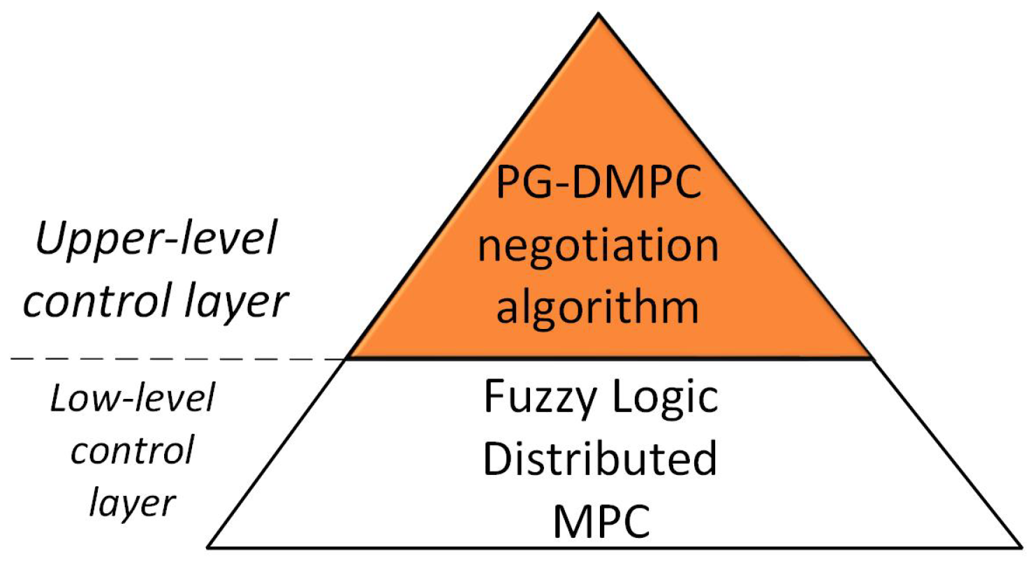
30]. Hence, it provides negotiation coefficients applied to the consensus of the global decisions through its pairwise local decisions to achieve the global goal and stability requirements of the FL-DMPC multi-agent control in the following control architecture (
Figure 1).
At each time instant t, a local decision is the control sequence defined as follows:
where
is the instant control action vector, and
is the prediction horizon of the local MPC controllers in the lower layer. The agent
i of the MPC with
of
N agents have local decisions
of
M pairwise negotiations in the FL-DMPC lower layer. To achieve a global decision
, it is proposed to agree as follows:
where
is the output of the deep neural network considered, like the negotiation coefficients weighing local decisions
, to achieve the control objective.
3. Methodology
Given a problem to be solved by the RL method, the environment is modelled as a Markov decision process with state space S, action space A, state transition function , with and , t as the time step, and a reward function . The training of an agent consists of the interaction of the agent with the environment, for which the agent sends an action to the environment, and it sends back a state and a reward as a qualifier of the according to the environment objectives. Consequently, each episode training generates an episode experience composed of the sequence with where T is the time horizon.
The PG algorithm selects
based on a stochastic policy
that assigns states to actions
. For this task, the algorithm uses a deep neural network as an approximation function of the stochastic policy
. The parameter of the policy optimization
is performed through the ascent optimization method of the gradient. This optimization aims to maximize for each state in the episode training for
, the discounted future reward,
where
is a discount factor, and
is the reward received at
t time step. Therefore, the objective function is
The score function allows optimization to be achieved without requiring the dynamic model of the system, optimizing the gradient of the logarithm of which expresses the probability that the agent selects given a .
The estimate of the discounted future reward
made by the Monte Carlo method has a high variance, leading to unstable learning updates, slow convergence, and thus slow learning of the optimal policy. The baseline method takes from
a value given from a baseline function
to address the variance in the estimate,
where
is called the advantage function. Consequently, the objective function becomes,
The exploration policy used by PG is based on a categorical distribution, where is a discrete probability distribution that describes the probability that the policy can take action a of a set k actions, with , given a state s, with the probability of each action listed separately and is the sum of the probabilities of all the actions equal to zero, .
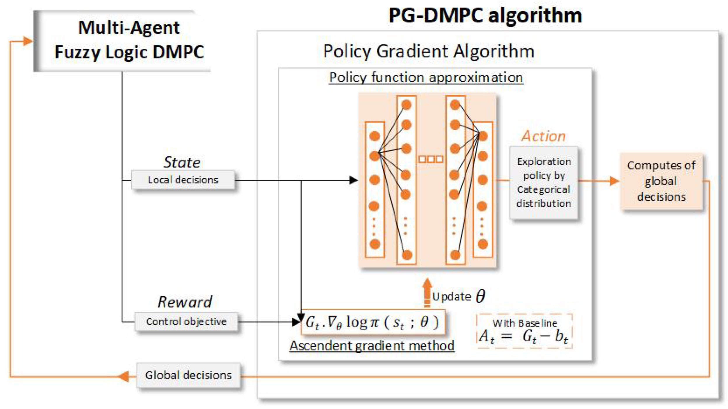
Figure 2 shows the policy gradient algorithm for the negotiating agent training. The optimization of deep neural networks is based on the input data collected at training by a categorical distribution exploration policy. Model knowledge is not necessary, only local decisions as the
state and control objectives as the
reward, a consequence of the
action of the previous
t time step employed to agree among the local decisions and obtain the global decisions of the agents.
3.1. PG-DMPC Algorithm
This section details the PG-DMPC algorithm implemented as a negotiating agent required for the upper layer of a distributed MPC control system. The aim of the upper layer PG-DMPC algorithm is to achieve a consensus among all candidate control sequences for each agent to obtain the final control action implemented.
In order to reach consensus, the deep neural network receives the available control sequences for each agent as state ,
where
,
N is the number of agents,
, and
is the total number of pairwise fuzzy negotiations in the lower layer performed by agent
i. The total number of control sequences received by the PG-DMPC upper level is defined as
. The states
, where
S is a compact subspace
.
The action
where
is a compact set,
are some coefficients weighting the control sequences to compute a suitable final control sequence
to be applied in the plant for agent
i, this procedure being the way to achieve consensus among agents in the upper layer. Particularly, the action vector is defined as
, where
,
. Note that for agent
i, the number of coefficients provided is
because the last one is obtained as the complement to 1 in order to reduce the computational load, and provided that
due to normalization when training the deep neural network,
Finally, the reward provided by the environment at each time step is defined in
Section 4.2.1 because it depends on the particular case study and its global control objective.
Considering states and actions defined above, Algorithm 1 developed negotiation in this paper is described:
| Algorithm 1 Proposed PG-DMPC negotiation algorithm for multiples agents |
At each time step t for each agent i: - 1.
The states are taken from the environment (low-level control layer) by the RL upper layer (deep neural network) defined by non-linear function . - 2.
The deep neural network takes the states as inputs in order to provide the actions which are the negotiation coefficients , for , , as outputs, The deep neural network outputs satisfy because it is a constraint considered at training for normalization. - 3.
The final control sequence is obtained, considering the actions provided by , . - 4.
The control sequences for each agent are aggregated to . is computed and compared with the global cost from the previous time t. Otherwise, the previous t control sequences that check stability, , are applied. Hence, the global cost function is
with the weighting matrices and and the terminal cost matrix , and the global state and input references is calculated by a procedure to remove offset based on [ 30].
|
The proposed PG-DMPC negotiation algorithm is performed in the upper-level control layer from the control architecture, (
Figure 1), where the low-level control layer is based on fuzzy logic DMPC and detailed in the next section.
3.2. Distributed MPC
The low-level control layer is a DMPC in which agent
negotiates with its neighbours in a pairwise manner. Local models are defined as:
where
denotes the time instant;
,
, and
are, respectively, the state, inputl and disturbance vectors of each subsystem
, constrained in the convex sets containing the origin in their interior
,
, respectively; and
,
and
are matrices of proper dimensions and can be seen in [
30].
The vector
represents the coupling with other subsystems
j belonging to the set of neighbors
, i.e,
where
is the input vector of subsystem
, and matrix
models the input coupling between
i y
j. Moreover,
is bounded in a convex set
due to the system constraints.
The linear discrete-time state-space model is
where
and
are the state vector and the input vector respectively,
is the disturbance vector, and
,
, and
are the corresponding matrices of the global system.
The low-level control layer performs the FL-DMPC algorithm for multiple agents. Specifically, fuzzy-based negotiations are made in pairs considering the couplings with their neighboring subsystems, which are assumed to hold their current trajectories. To this end, it a shifted sequence of agent
i is used, which is defined by adding
on the sequence chosen at the previous time step
:
To make the paper self-contained, a brief description of the FL-DMPC algorithm [
30] is presented here (Algorithm 2):
| Algorithm 2 Multi-agent FL-DMPC algorithm |
At each time step t for each agent i - 1.
Firstly, agent i measures its local state and disturbance . - 2.
Agent i calculates its shifted trajectory and sends it to its neighbors. - 3.
Agent i minimizes its cost function considering that neighbor applies its shifted trajectory . It is assumed that the rest of the neighboring subsystems follows their current control trajectories . Specifically, agent i solves
subject to
Constraints
where set is imposed as the terminal state constraint of agent i. Details regarding the calculation are given in [ 30].
|
- 4.
Agent i again optimizes its cost maintaining its optimal input sequence to send to find the input sequence wished for its neighbors . Here, it is also assumed that subsystems l follow their current trajectories. To this end, agent i solves
subject to
- 5.
Agent i sends to agent j and receives . - 6.
For each agent , the triple of possible inputs is . Since the wished control sequence is computed by neighbor j without considering state constraints of agent i, it is needed to check whether state constraint satisfaction of agent i holds after applying . Otherwise, it is excluded from the fuzzification process. Afterwards, fuzzy negotiation is applied to compute the final sequence . Similarly, is computed. - 7.
A resulting pairwise fuzzy negotiation sequence is defined based on and , assuming that the rest of subsystem follows their pre-defined trajectories. - 8.
Agent i sends its cost for the fuzzy and stabilizing control inputs to its neighbours and vice versa. Let us define ; if the condition
holds, then stability is guaranteed, and thus, is sent to the upper control layer. Otherwise, is sent.
|
Hence, the cost function
is
with
being a semi-positive definite matrix,
,
being positive-definite matrices, and
and
being the state and input references calculated by a procedure to remove offset based on [
30].
4. Case Study
This section describes the coupled eight-tank plant based on the quadruple tank process in which the proposed PG-DMPC algorithm was implemented together with the previously detailed low-level control layer.
4.1. Plant Description and Control Objective
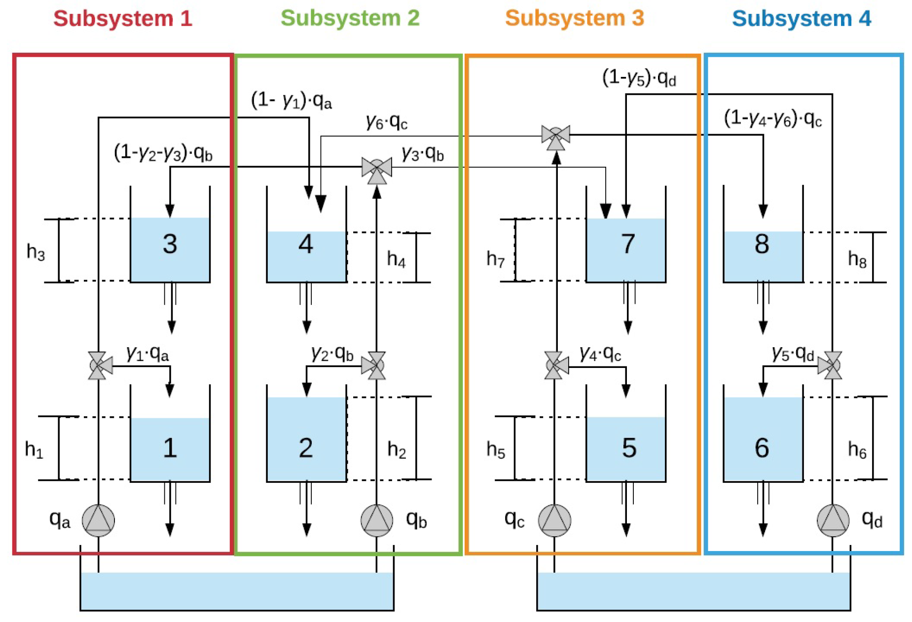
The eight-coupled tanks plant comprises eight interconnected tanks (
Figure 3) with four upper tanks (3, 4, 7, and 8) that discharge into the lower ones (1, 2, 5, and 6), which in turn, discharge into sinking tanks. The plant is controlled by four pumps whose flows are divided through six three-way valves
with
manually operated.
The system is divided into s subsystems with : Tanks 1 and 3 are part of Subsystem 1; Tanks 2 and 4 form Subsystem 2; Tanks 5 and 7 belong to Subsystem 3; and the rest of the tanks form Subsystem 4. The level of Tank with , being the controlled variables the levels , , , and renamed as, , , , and for each agent. The manipulated variable is the flow given by the pump of each Subsystem s. The tank level operating point is established, for as , , , , , , , (units: meters). In addition, the operating point of the flow of the pumps as , , , (units: m3/h).
The aggregated state vector and input state vector are defined as
The disturbance state vector is defined as .
The control objective is to solve a tracking problem to reach the reference ,
, where
is the target level of the controlled variable
.
For the upper tank levels, the objective is to keep the operating point despite the disturbance affecting the system. Additionally, the state and input vectors are constrained by
The linear state space models of the global system and subsystems are detailed in [
30].
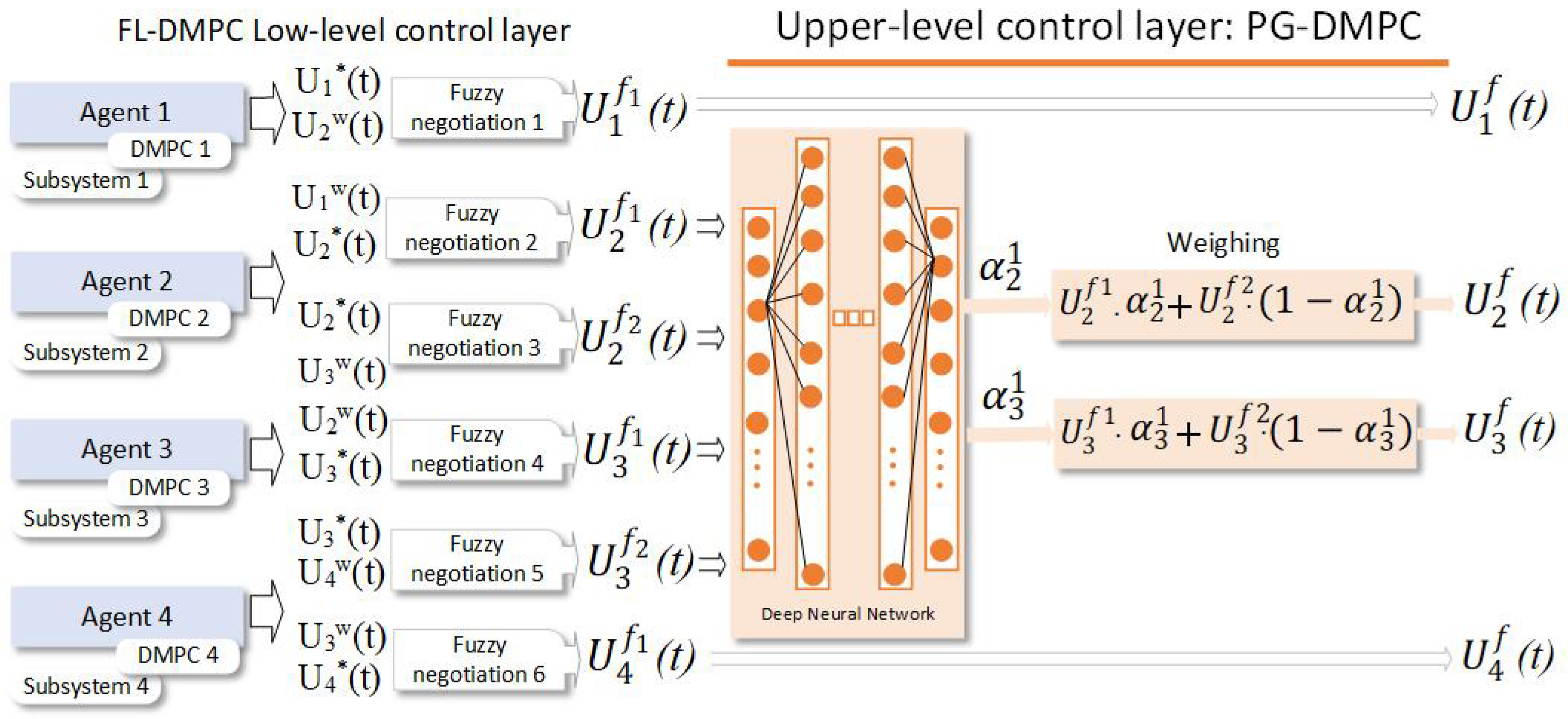
4.2. Negotiation Framework
In this case study, there are four agents. Subsystems 1 and 4 have only one neighbour, Subsystems 2 and 3, respectively, because coupling only exists with them. On the other hand, Subsystems 2 and 3 have two neighbours each. Then, the low-level control layer FL-DMPC provides agent
i the following control sequences
,
,
, and
, obtained by performing pairwise negotiation among agents. In particular,
, and
in (Equation (
1)).
Due to the particular configuration of the eight coupled tanks system, negotiation is not required in the upper layer for Subsystems 1 and 4, and therefore
and
. Negotiation is only needed for Agents 2 and 3, and the state is defined as:
The actions
provided by the deep neural network are:
where
and
. Note that only one weighting coefficient is obtained for each subsystem because the other ones are directly obtained from:
Therefore, considering that the final sequence for each agent is , with the prediction horizon for each local MPC controller and manipulated variable, , to be applied to the system is selected as the first value of the sequences, usually an MPC framework:
, , ,
Figure 4 displays the implemented PG-DMPC algorithm within the control architecture performed in the case study, where PG-DMPC receives local decisions from a FL-DMPC and gives global decisions according to the control objective.
4.2.1. Reward
The PG algorithm optimizes weights
of the deep neural network
used as an approximation function of the stochastic policy
in order to maximize the discounted future reward
(Equation (
2)). The
reward function is critical for the proper working of the RL, and it is defined heuristically as:
where
is the tracking square error, and
is the error threshold for each subsystem. Note that a positive reward corresponds to a desired situation and negative rewards penalties for the RL.
The maximum reward is given when the tracking error does not exceed the threshold value for any subsystem and the weighting coefficient provided by the deep neural network belongs to
. A small penalty is given when any error exceeds the threshold, but still,
and
. Finally, a large penalty defined by
is added if
or
in order to obtain normalized values for the coefficients:
4.2.2. Discrete Action Framework
Discretization is the process of transferring continuous functions, models, variables, and equations to discrete counterparts. In our case, the actions of the trading agent are discrete values, which in Equations (
20) and (
21) give a discrete weight to the continuous sequences for consensus. More specifically, the discretization is carried out as
, whit
. A discrete action framework is employed to obtain a shorter training time, simpler calculations, a lower computational cost, and faster convergence. According to discrete stochastic policy, each output of the deep neural network is the probability of assigning a combination of discrete values of
and
given a specific state in the inputs.
4.3. Training
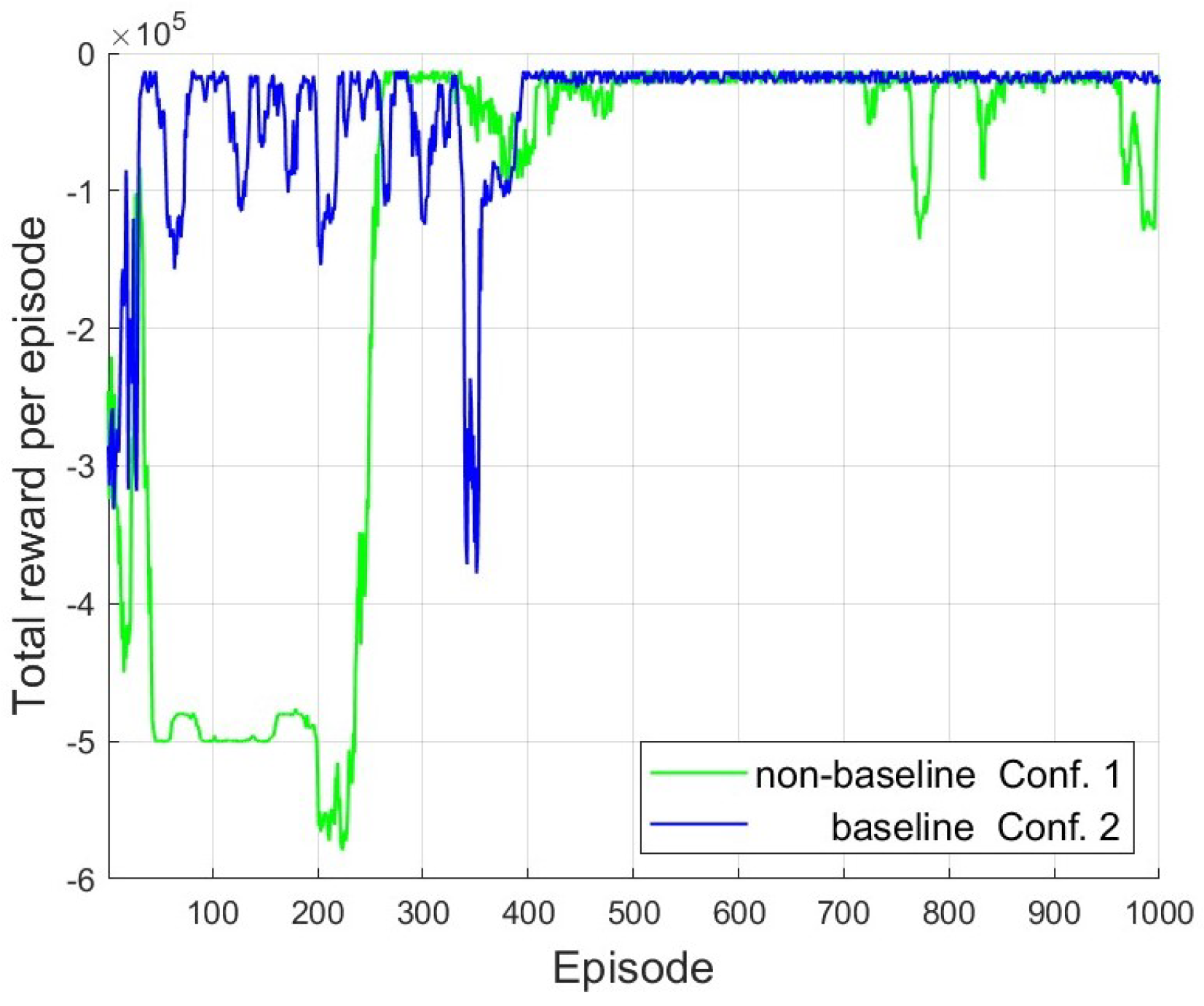
This section compares the influence of the baseline method with two approaches, the convergence velocity and stability, during the search for the optimal policy.
Table 1 shows the two PG configurations compared and trained.
Policy and baseline networks employed as approximation functions are set up to a 0.01 fixed learning rate using the Adam optimizer. The policy deep neural network consists of three fully connected hidden layers, whereas the baseline network uses one fully connected hidden layer.
Training and results are obtained using the MATLAB reinforcement learning toolbox. The two configurations trained for 1000 episodes with the time horizon and the simulation of the environment with sample time . Consequently, each is an RL training time step. The initial randomization of levels taken from the interval is required and performed. As a remark, although the agents trained with the exploratory policy based on categorical distribution, their policies during validation follow greedy exploration, which selects the action with maximum likelihood.
Figure 5 displays the non-use and use of the baseline method under the categorical distribution exploration policy. Baseline and non-baseline in policy convergence have quite a similar approach time to the high rewards zone. Despite this, the baseline case sets more stability and a faster approach to the high-reward zone.
4.4. Performance Indexes
In order to evaluate the proposal, the following performance indexes were established.
MPC global cost function,
where
is detailed in Equation (
7).
Sum of the integrals of squared errors of controlled levels,
with
The sum of the squared differences of the controlled levels
is,
The sum of the pumping energies
for each pump
s as the sum of the average of pumping energy over the prediction horizon is proportional to water flows provided by the pumps:
with
with
for all performance indexes.
5. Results
Results of the proposed PG-DMPC are presented in this section. The objective of the PG-DMPC algorithm is to provide consensus among local decisions from an FL-DMPC algorithm to achieve control objectives. The proposal PG-DMPC is compared with fuzzy DMPC (FL) [
30], DMPC using a cooperative game [
31], and the centralized MPC. FL and Coop. The game was also implemented in the upper layer. Furthermore, the influence of the baseline method is evaluated. Three validation cases (
Table 2) were employed to demonstrate the proper performance of the proposal under the different initial, reference state vectors and disturbance states. The sampling time used in simulations is
s.
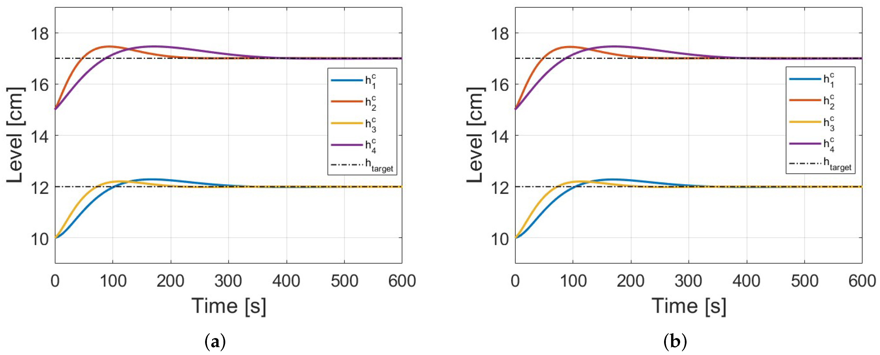
Case 1: The reference vector is the same as the one used for training, and the state vector of the operating point was considered as the initial state vector, .
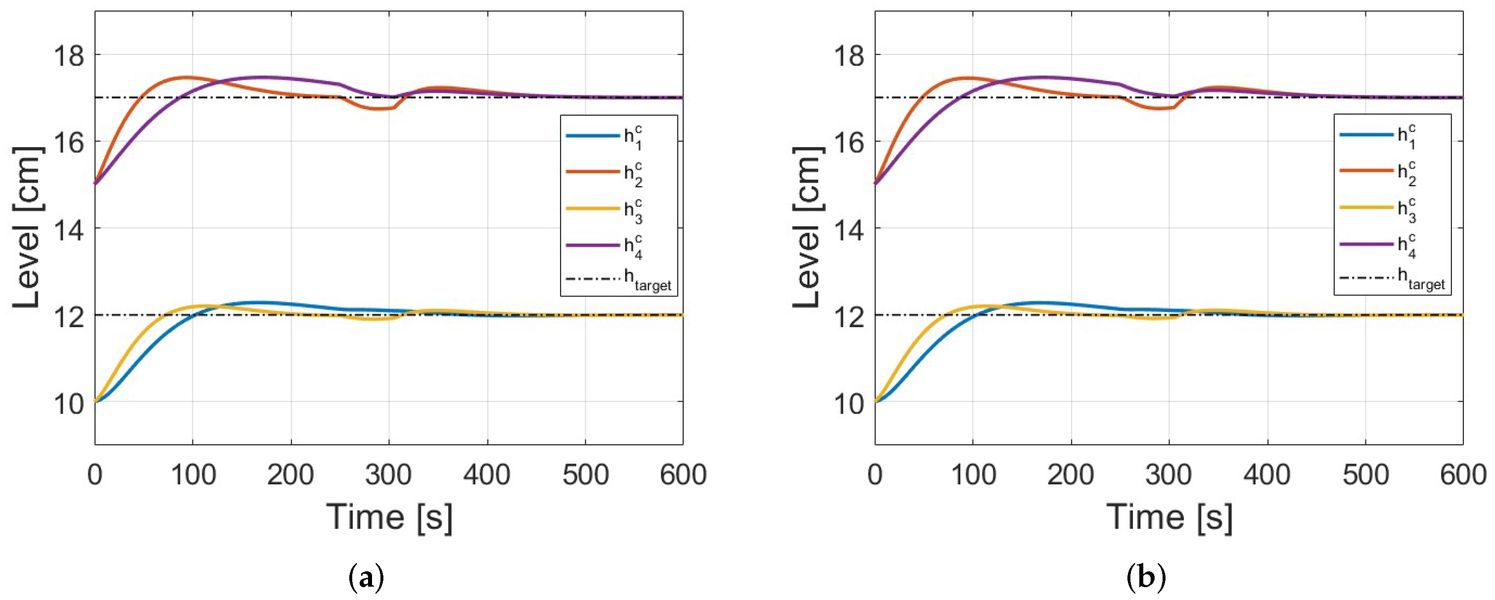
Case 2: The reference vector and the initial state vector are the same as those used in Case 1, but for this case, the disturbances were included.
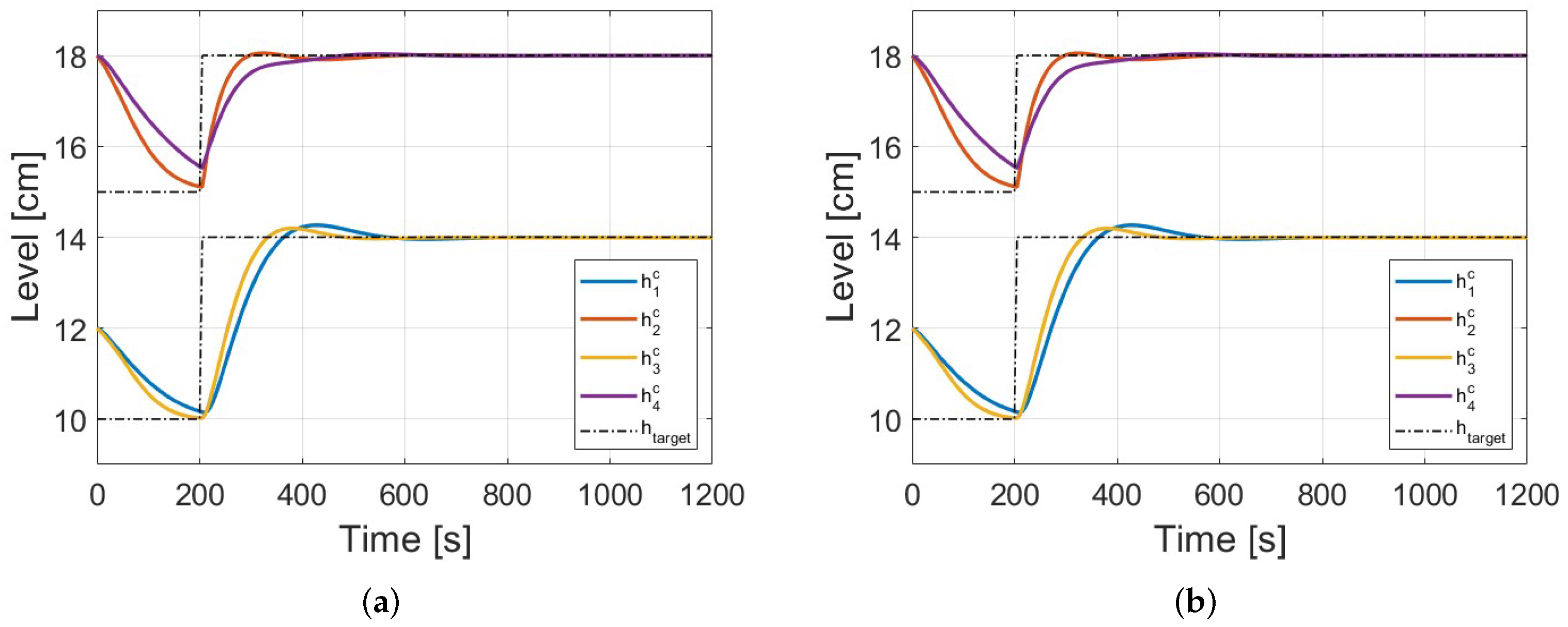
Case 3: The reference vector changes at from the operation point as initial reference vector to with , , , . The initial state vector was taken from . Note that the initial state vector is taken out of the interval for initial state vectors during training.
Table 3,
Table 4 and
Table 5 show the performance of the proposal and the techniques considered in Cases 1, 2, and 3, respectively. In the same order as the validation cases,
Figure 6,
Figure 7 and
Figure 8 portray the evolution of the state vectors until the reference vector is reached by Conf. 1 and Conf. 2.
Table 3,
Table 4 and
Table 5 show that the centralized control has the best results because it has the availability of full plant information for prediction. For validation Case 1, Coop game offers better results in Pe, ISE, and e. Both configurations of the PG-DMPC show an advantage in
over the FL, while
ISE and
e display very close values to FL. (
Table 3).
In validation Case 2, Coop. game shows better
than PG-DMPC and FL techniques. In this case, the worst
are given by PG-DMPC. On the other hand, these three techniques show
ISE and
e are very close to each other. Although the measure disturbance was added, an acceptable response was raised by PG-DMPC (
Table 4).
Finally, in Case 3, the Coop game and FL show better
values. At the same time, the worst of
ISE and
e are given by FL. The two PG-DMPC configurations display similarly in the four indices. The PG-DMPC agent has an acceptable response and is comparable to the other techniques even though it was not trained for reference tracking (
Table 5).
In addition,
Table 6 shows the compliance of the stability evaluation according to Step 4 of Algorithm 1 (see
Section 2). For each configuration and validation case, the percentage of total time that cost
decreases without using the backup sequence
is shown in the table. Both configurations show similar stability, highlighting the stability in Case 2 under Conf. 2.


