Article

Random Orthogonal Search with Triangular and Quadratic Distributions (TROS and QROS): Parameterless Algorithms for Global Optimization

by
Bruce Kwong-Bun Tong
1,2,*,
Chi Wan Sung
3 and
Wing Shing Wong
2
1
Department of Electronic Engineering and Computer Science, Hong Kong Metropolitan University, Hong Kong, China
2
Department of Information Engineering, The Chinese University of Hong Kong, Hong Kong, China
3
Department of Electrical Engineering, City University of Hong Kong, Hong Kong, China
*
Author to whom correspondence should be addressed.
Appl. Sci. 2023, 13(3), 1391; https://doi.org/10.3390/app13031391
Submission received: 13 December 2022 / Revised: 6 January 2023 / Accepted: 7 January 2023 / Published: 20 January 2023
(This article belongs to the Special Issue Evolutionary Computation: Theories, Techniques, and Applications)

Abstract

:
In this paper, the behavior and performance of Pure Random Orthogonal Search (PROS), a parameter-free evolutionary algorithm (EA) that outperforms many existing EAs on the well-known benchmark functions with finite-time budget, are analyzed. The sufficient conditions to converge to the global optimum are also determined. In addition, we propose two modifications to PROS, namely Triangular-Distributed Random Orthogonal Search (TROS) and Quadratic-Distributed Random Orthogonal Search (QROS). With our local search mechanism, both modified algorithms improve the convergence rates and the errors of the obtained solutions significantly on the benchmark functions while preserving the advantages of PROS: parameterless, excellent computational efficiency, ease of applying to all kinds of applications, and high performance with finite-time search budget. The experimental results show that both TROS and QROS are competitive in comparison to several classic metaheuristic optimization algorithms.

1. Introduction

Black-box optimization refers to optimizing an objective function in the absence of prior knowledge of the function. The only knowledge of the objective function is the observed outputs of the given inputs. Metaheuristics such as evolutionary computation (EC) techniques and evolutionary algorithms (EAs) are widely employed for black-box optimization of various fields across science and engineering [1,2,3] due to their certain primary advantages over the traditional techniques (such as Newton’s method and gradient descent) including high robustness in solving complex real-world problems, and domain knowledge and regularity (e.g., convexity, continuity, differentiability) of the functions to be optimized are generally not required [4].
However, these algorithms often require a large number of function evaluations to evolve or update the candidate solutions in order for errors reduced to a satisfactory level [5]. For many real-world problems, evaluating the objective function is often costly. These function evaluations may involve conducting computational intensive numerical simulations or expensive physical experiments [6,7,8,9] When only a limited number of objective function evaluations is affordable, EC’s trial and error approach becomes unattractive.
Moreover, EC techniques are commonly recognized as heuristic search algorithms because their theoretical analysis often lags behind the development of the algorithms [4,10]. Their performance is often sensitive to the problem-dependent hyper-parameters [11]. Various approaches have been suggested to overcome these drawbacks. For example, building an inexpensive surrogate model for evaluation so as to reduce the number of objective function evaluations [5,12], and automatic or self-adaptive tuning of the hyper-parameters [11,13,14].
In this paper, we propose two algorithms for expensive black-box optimization. The two algorithms are modified from Pure Random Orthogonal Search (PROS) [15]. PROS is a (1 + 1) Evolutionary Strategy ((1 + 1) ES), a kind of EA, that has only one parent in the population and generates one child in each generation that competes with its parent. The finite-time performance of PROS is promising and outperforms several existing EC techniques on most benchmark functions [15]. Unlike those well known EAs, PROS is free of parameters and thus the tuning of parameters is not required. To the best of our knowledge, there were no mathematical analyses on the behaviour and performance of the algorithm reported in the literature. In this paper, we aim to fill this gap. The major contributions of this research work are summarized as follows:
1.
The behavior and performance analysis of PROS, which are not available in [15], are provided here.
2.
Two effective novel (1 + 1) ES based on PROS, namely TROS and QROS, are proposed and they outperform PROS on a set of benchmark problems.
3.
The performance of TROS and QROS are found competitive with three well-known optimization algorithms (GA, PSO and DE) on a set of benchmark problems.

Problem Formulation

In this paper, we restrict attention to global optimization of expensive black-box functions. The goal of global optimization is to find x * which is a global minimum of f,
x * = arg min x Ω f ( x )
where f : R D R is a scalar-valued objective function defined on the decision space Ω R D and x = ( x 1 , x 2 , . . . , x D ) represents a vector of decision variables with D dimensions.
We have made the following assumptions.
Assumption 1.
f has a single global optimum f * = min x Ω f ( x ) .
Assumption 2.
f can be evaluated at all points of Ω in an arbitrary order.
Assumption 3.
The slope of f is bounded with a Lipschitz constant L such that
| f ( x 1 ) f ( x 2 ) | L x 1 x 2 , x 1 , x 2 Ω ,
where L > 0 and · denotes the Euclidean norm.
It has to be noted that although f is assumed a Lipschitz function, the corresponding Libschitz constant L is unknown to an optimization algorithm.

2. Analysis of the Pure Random Orthogonal Search (PROS) Algorithm

The PROS algorithm was originally proposed by Plevris et al. in [15]. We describe it with our revised notation as follows:
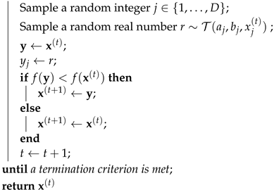
Initially, a candidate solution vector x ( 0 ) is generated randomly from Ω (lines 1 and 2). Then, for each iteration t, j is chosen randomly from 1 to D (line 4) and a real number r is drawn randomly with uniform distribution within the search space of the j-th decision variable (line 5). A new candidate solution vector y is obtained by replacing the value of the j-th decision variable of the current best solution vector x ( t ) with r (lines 6 and 7). The new candidate solution vector y is evaluated and the new best solution vector x ( t + 1 ) is then updated based on the comparison result between f ( y ) and f ( x ( t ) ) . If f ( y ) is smaller, y is accepted as the new best solution vector. Otherwise, y is rejected (lines 8 to 12). The iteration counter t is updated and the search process is repeated until a termination criterion is met (lines 13 and 14). Finally, the best solution vector found by the algorithm is returned as the final result (line 15).
In the following analysis, we assume the algorithm runs continuously until the global optimum is found (defined below of this section). It is because we are interested in analyzing its ultimate performance. In practice, it may take an infinitely long time to reach the global optimum. Therefore, other termination criteria are usually adopted. For example, the algorithm stops when no improvement is made after a certain number of iterations or when a pre-defined maximum number of iterations is reached.
The error of the algorithm after running for t iterations is given by
e t = f ( x ( t ) ) f ( x * ) .
Here, x ( t ) is the solution vector found by the algorithm in the t-th iteration and is also the best solution vector found by the algorithm after t iterations. It is because the values of the solution vectors found by PROS is monotonically non-increasing. That is,
f ( x ( t ) ) f ( x ( t 1 ) ) f ( x ( 0 ) ) ,
Consider the pseudo code from line 8 to line 12 of Algorithm 1. In the t-th iteration, when a better solution y is found, it will be assigned to x ( t + 1 ) . In this case, f ( x ( t + 1 ) ) < f ( x ( t ) ) . When no better solution is found in the t-th iteration, x ( t ) will be assigned to x ( t + 1 ) . In this case, f ( x ( t + 1 ) ) = f ( x ( t ) ) . Combining the two conditions, f ( x ( t + 1 ) ) f ( x ( t ) ) and the inequalities then follow.
Algorithm 1: Pure Random Orthogonal Search (PROS)
input: nil
output: the best solution vector x ( t ) found by the algorithm
t 0
Initialize x ( t ) = ( x 1 , x 2 , , x D ) randomly from
Ω = [ a 1 , b 1 ] × [ a 2 , b 2 ] × × [ a D , b D ]
repeat

   Applsci 13 01391 i001
Definition 1.
(Region of Global Optimum). It is said that a candidate solution vector x is in the region of global optimum R ϵ if the error of x is not larger than ϵ. That is,
R ϵ = { x : x Ω and f ( x ) f * ϵ } ,
where ϵ is a small positive real number denoting the tolerance of error.
Definition 2.
(Convergence Time). The convergence time T of an algorithm is defined to be the first time t when
x ( t ) R ϵ .

2.1. One-Dimensional Functions

In this section, we study the performance of PROS on one-dimensional functions defined on the domain Ω = [ a , b ] . Since we are interested in the case where ϵ is small, we assume that 2 ϵ L < b a .
Lemma 1.
For any ϵ > 0 , the region of the global minimum contains an interval of minimum length ϵ L for all one-dimensional functions.
Proof. 
Let x * = ( x 1 * ) be the global optimum, x l = ( x 1 l ) R ϵ be a point on the left of x * and x r = ( x 1 r ) R ϵ be a point on the right of x * . We are going to find a sufficient condition to ensure that [ x 1 l , x 1 r ] is in the region of global optimum. Since f is a Lipschitz function, the interval [ x 1 l , x 1 * ] belongs to R ϵ if x 1 l satisfies
f ( x l ) f ( x * ) L x l x * = L ( x 1 * x 1 l ) ϵ ,
or equivalently, x 1 l x 1 * ϵ L . We want to make x 1 l as small as possible, so we let
x 1 l = max { a , x 1 * ϵ L } .
Similarly, the interval [ x 1 * , x 1 r ] belongs to R ϵ if
x 1 r = min { b , x 1 * + ϵ L } .
Since we have assumed 2 ϵ L < b a , it is impossible that x 1 l = a and x 1 r = b hold simultaneously. Therefore, at least one of the intervals has length ϵ L . Hence, the length of the region of global optimum is at least ϵ L . □
Theorem 1.
The expected convergence time of PROS for one-dimensional functions is bounded above by L ( b a ) ϵ .
Proof. 
Let l be the length of the region of global optimum, R ϵ . The probability that a point chosen uniformly at random falls in R ϵ is given by
p = l b a ϵ L ( b a ) .
The convergence time T is geometrically distributed with parameter p. Its expected value is given by
E [ T ] = 1 p L ( b a ) ϵ .
Corollary 1.
PROS converges in probability to the region of global optimum for all one-dimensional functions, i.e.,
lim t P { x ( t ) R ϵ } = 1 , ϵ > 0 .
Proof. 
For any realization { x ( t ) : t = 0 , 1 , 2 , } , f ( x ( t ) ) is monotonically non-increasing in t. If x ( t ) R ϵ , then x ( t + τ ) R ϵ for all non-negative integer τ . Therefore, P { x ( t ) R ϵ } is monotonically non-decreasing in t. Since the sequence is bounded above by 1, it is convergent.
Given any ϵ > 0 , the expected convergence time is bounded according to Theorem 1. If lim t P { x ( t ) R ϵ } was non-zero, then the expected convergence time would be unbounded, which leads to a contradiction. □

2.2. Multi-Dimensional Functions

In this section, we study the performance of PROS on D-dimensional functions with domain Ω = [ a 1 , b 1 ] × [ a 2 , b 2 ] × × [ a D , b D ] , where D > 1 . In particular, we focus on the class of totally separable functions as defined below. For notation simplicity, define x i ( x 1 , x 2 , , x i 1 , x i + 1 , , x D ) .
Definition 3.
(Partially Separable Function). A function f ( x ) is partially separable with coordinate i if arg min x i f ( x i , x i ) is independent of x i .
An example of partially separable functions with coordinate i = 1 is:
f ( x ) = x 1 2 + i = 2 D 1 ( x i x i + 1 ) 2 .
Definition 4.
(Totally Separable Function). A function f ( x ) is totally separable if it is partially separable with every of the D coordinates.
An example of totally separable functions is:
f ( x ) = i = 1 D ( x i 2 + 1 ) .
In each iteration, PROS minimizes f in one of the random coordinate i. As f is totally separable, each coordinate i can be minimized independently. The following result shows that PROS converges to the region of global optimum in probability.
Theorem 2.
PROS converges in probability to the region of global optimum for all totally separable functions, i.e.,
lim t P { x ( t ) R ϵ } = 1 , ϵ > 0 .
Proof. 
Since f is Lipschitz, given any x i , we have
| f ( x i , x i ) f ( x ˜ i , x i ) | L | x i x ˜ i | .
Therefore, f can be regarded as a one-dimensional Lipschitz function in x i with the same constant L. As shown in the previous subsection, there is an interval V ϵ i of minimum length ϵ i L such that for all x i V ϵ i ,
| f ( x i , x i ) f ( x i * , x i ) | ϵ i .
Note that V ϵ i is independent of x i . Under PROS, it is clear that
lim t P { x i ( t ) V ϵ i } = 1 , ϵ i > 0 .
Since f is Lipschitz, it is a continuous function. Given any ϵ > 0 , there exists sufficiently small positive ϵ i ’s such that when x i ( t ) V ϵ i for all i, we must have x ( t ) R ϵ . The statement then follows from
P { x ( t ) R ϵ } P { x i ( t ) V ϵ i , i } = i = 1 D P { x i ( t ) V ϵ i } .
The expected convergence time can be obtained for the following subclass of totally separable functions.
Definition 5.
(Additively Separable Function). A function f is additively separable if f ( x ) can be written in the form of f 1 ( x 1 ) + f 2 ( x 2 ) + + f D ( x D ) , where x = ( x 1 , x 2 , , x D ) and f 1 , f 2 , , f D are one-dimensional functions.
An example of additively separable functions is the sum-of-spheres function:
f s p h e r e ( x ) = i = 1 D x i 2 .
For the optimization of D-dimensional additively separable functions, it is equivalent to optimize D one-dimensional functions independently, i.e.,
min x Ω f ( x ) = i = 1 D min x i [ a i , b i ] f i ( x i ) .
Theorem 3.
The expected convergence time of PROS for D-dimensional additively separable functions is bounded above by
E [ T ] D 2 L ϵ i = 1 D ( b i a i ) .
Proof. 
A point x = ( x 1 , x 2 , , x D ) belongs to R ϵ if
i = 1 D ( f i ( x i ) f i * ) ϵ ,
where f i * is the global minimum of the i-th one-dimensional function. Then,
f i ( x i ) f i * ϵ D , for i { 1 , , D }
is a sufficient condition for x R ϵ .
Let S i be the iteration time PROS enters the region for x i as stated in (1). Under PROS, at each iteration t, the coordinate to be optimized is chosen uniformly at random. As in the proof of Theorem 1, S i is a geometric random variable with parameter
p i 1 D ϵ / D L ( b i a i ) = ϵ D 2 L ( b i a i ) .
Note that S i ’s are not independent. We bound the convergence time T as follows:
T max { S 1 , , S D } S 1 + + S D .
Hence,
E [ T ] i = 1 D E [ S i ] = i = 1 D 1 p i D 2 L ϵ i = 1 D ( b i a i ) .

3. Modified PROS with Local Search Mechanism

Although the PROS algorithm converges to the global optimum, provided that the sufficient conditions are satisfied, it converges slowly when compared with other well-known EC algorithms [15]. The major reason is PROS simply performs uniform orthogonal search in every iteration with no local search mechanism. The probability of finding an improved solution (defined in the below subsection) diminishes as it moves closer to the global optimum. Consider the situation that in the t-th iteration, x ( t ) is already very close to x * but has not yet fallen into in the region of global optimum. There is a high chance that x ( t + 1 ) would reach the region of the global optimum if a narrow-range local search is performed in the ( t + 1 ) -th iteration. However, with uniform orthogonal search, the chance to reach the global optimum is relatively low, thus making it converge slowly. One may consider using a sampling policy other than uniform to perform local search.

3.1. Triangular-Distributed Random Orthogonal Search (TROS)

In this section, we present our first proposed algorithm called Triangular-Distributed Random Orthogonal Search (TROS). The TROS algorithm (Algorithm 2) is presented as follows:
Algorithm 2: Triangular-Distributed Random Orthogonal Search (TROS)
input: nil
output: the best solution vector x ( t ) found by the algorithm
t 0
Initialize x ( t ) = ( x 1 , x 2 , , x D ) randomly from
  Ω = [ a 1 , b 1 ] × [ a 2 , b 2 ] × × [ a D , b D ]
repeat

   Applsci 13 01391 i002
Compared with PROS, TROS has one change in line 5 of Algorithm 1. Instead of sampling the next point of the j-th decision variable using uniform distribution, the triangular distribution T is used in the TROS algorithm. The probability density function of the triangular distribution T ( a , b , c ) is
f T ( x ) = 2 b a x a c a , a < x c 2 b a b x b c , c < x < b 0 , x a or x b
where a, b and c are the parameters of the distribution that represents the lower limit of x, upper limit of x and mode of x, respectively. The triangular distribution is illustrated in Figure 1.
In each iteration of TROS, the next point is sampled using the triangular distribution with the settings a = a j , b = b j , c = x j ( t ) where j { 1 , 2 , , D } is the randomly chosen decision variable for the current iteration, a j and b j are the lower bound and upper bound of the j-th decision variable, and x j ( t ) is the value of the j-th decision variable of the current best solution vector. With this distribution, there is a higher chance to draw a sample that is near to the current position x j ( t ) than is far from the current position. As a result, the algorithm performs exploitation (that is, encourages local search) on the j-th decision variable.

3.2. Quadratic-Distributed Random Orthogonal Search (QROS)

In this section, we present our second proposed algorithm called Quadratic-Distributed Random Orthogonal Search (QROS). The QROS algorithm (Algorithm 3) is presented as follows:
Algorithm 3: Quadratic-Distributed Random Orthogonal Search (QROS)
input: nil
output: the best solution vector x ( t ) found by the algorithm
t 0
Initialize x ( t ) = ( x 1 , x 2 , , x D ) randomly from
  Ω = [ a 1 , b 1 ] × [ a 2 , b 2 ] × × [ a D , b D ]
repeat

   Applsci 13 01391 i003
Compared with TROS, QROS has one change in line 5 of Algorithm 2. The value of the j-th decision variable is sampled using the quadratic distribution Q . The probability density function of the quadratic distribution Q ( a , b , c ) is
f Q ( x ) = α Q ( x a ) 2 , a < x c β Q ( x b ) 2 , c < x < b 0 , x a or x b
where α Q = 3 ( b a ) ( c a ) 2 , β Q = 3 ( b a ) ( c b ) 2 , a, b and c are the lower limit of x, upper limit of x and mode of x, respectively. The quadratic distribution is illustrated in Figure 1.
In each iteration of QROS, the next point is sampled using the quadratic distribution with the settings a = a j , b = b j , c = x j ( t ) where j { 1 , 2 , , D } is the randomly chosen decision variable for the current iteration, a j and b j are the lower bound and upper bound of the j-th decision variable, and x j ( t ) is the value of the j-th decision variable of the current best solution vector. With this distribution, there is a higher chance to draw a sample that is near to the current position x j ( t ) than is far from the current position. Compared with TROS, QROS encourages exploitation even more than TROS.
It has to be noted that both TROS and QROS are still “parameter-free” algorithms, as a and b are fixed boundaries, and c is determined based on the current best solution vector. With a simple modification, both TROS and QROS are able to improve the convergence speed of PROS and keep the major properties of PROS: parameterless, excellent computational efficiency, easy to apply to all kinds of applications, and high performance with finite-time search budget.

3.3. Analysis of the Modified Algorithms

In this subsection, we are going to explain the motivation and analyze the performance of the two algorithms. Sampling using uniform distribution can be considered as performing global search on a decision variable, while sampling using the triangular distribution and the quadratic distribution can be considered as performing local search on a decision variable.
Definition 6.
(Improved Solution). The candidate solution vector x ( t + 1 ) found by the algorithm is said to be improved if its error is less than the error of the current best solution. That is,
f ( x ( t + 1 ) ) f ( x * ) < f ( x ( t ) ) f ( x * )
or simply
f ( x ( t + 1 ) ) < f ( x ( t ) )
where t denotes the current iteration.
For continuous (or Lipschitz) unimodal functions defined on a bounded domain, finding an improved solution vector always lead to the convergence to the global optimum. However, it may not be true for multimodal functions. Therefore, we are not interested in simply finding an improved solution vector. Here, we define a restrictive subset of improved solution vectors.
Definition 7.
(Tame Solution). The candidate solution vector x ( t + 1 ) found by the algorithm is said to be a t a m e solution if the errors of all points in between the line containing the candidate solution and the optimum solution are all less than the error of the current best solution. That is,
f ( α x ( t + 1 ) + ( 1 α ) x * ) < f ( x ( t ) ) , α [ 0 , 1 ]
where t denotes the current iteration.
A local optimum in a multimodal function is not considered as a t a m e solution if there exists a high hill in between the local optimum and the global optimum. The purpose of defining t a m e solution is when a t a m e solution is found, it does not only mean the solution is improved but also implies one could apply some simple techniques to converge to the global optimum. Therefore, we are interested in knowing the probability of finding a t a m e solution by each of the algorithms.
We define following terms for the analysis of the performance of the proposed algorithms. Let x ( t ) = ( x 1 ( t ) , x 2 ( t ) , , x D ( t ) ) be the current best solution vector, and j { 1 , , D } be the chosen decision variable of the current iteration. Given x j ( t ) = ( x 1 ( t ) , , x j 1 ( t ) , x j + 1 ( t ) , , x D ( t ) ) , assume f ( x j ( t ) , x j ) has a unique global minimum and is denoted as x j * . That is,
f ( x j ( t ) , x j * ) f ( x j ( t ) , x j ) , x j [ a j , b j ] .
Let R j be the set of values of the j-th decision variable that belong to improved solution vectors. That is,
R j = { x j | f ( x j ( t ) , x j ) < f ( x j ( t ) , x j ( t ) ) , x j [ a j , b j ] } .
Let S j be the set of values of the j-th decision variable that belong to t a m e solution vectors. That is,
S j = { x j | ( α x j + ( 1 α ) x j * ) R j , α [ 0 , 1 ] , x j [ a j , b j ] } .
Let x j l be the smallest x j value and x j r be the largest x j value of the t a m e solutions, respectively. That is,
x j l = inf S j
and
x j r = sup S j .
Let l j be the length of the interval S j . That is,
l j = x j r x j l .
By Lemma 1, l j is non-negative and is bounded below by
l j e L
where e is the error of f ( x j ( t ) , x j ( t ) ) with respect to f ( x j ( t ) , x j * ) . That is,
e = f ( x j ( t ) , x j ( t ) ) f ( x j ( t ) , x j * ) .
Figure 2 shows two examples of multimodal functions with the corresponding set of t a m e solutions denoted by S j .
Definition 8.
(Probability of T a m e Convergence). The probability of t a m e convergence is defined as the probability of an algorithm with sampling policy π to find a t a m e solution in its next iteration, given the current best solution vector. That is,
P { x j ( t + 1 ) S j | x ( t ) , x j ( t + 1 ) π x ( t ) } .
Lemma 2.
The probability of t a m e convergence of PROS is l j b j a j .
Proof. 
Let P j U be the probability that a t a m e solution is found by sampling using uniform distribution on the j-th decision variable in the ( t + 1 ) -th iteration, given the best solution vector in the t-th iteration. Then
P j U = P { x j ( t + 1 ) S j | x j ( t ) , x j ( t + 1 ) U ( a j , b j ) } = l j b j a j .
Theorem 4.
The probability of t a m e convergence of TROS is l j b j a j ( l j + 2 v j u j + l j + v j ) when x j ( t ) < x j * and is l j b j a j ( l j + 2 q j q j + l j + r j ) when x j ( t ) > x j * where u j = x j l x j ( t ) , v j = b j x j r , q j = x j l a j and r j = x j ( t ) x j r .
Proof. 
Let P j T be the probability that a t a m e solution is found by sampling using the triangular distribution on the j-th decision variable in the ( t + 1 ) -th iteration, given the best solution vector in the t-th iteration. That is,
P j T = P { x j ( t + 1 ) S j | x j ( t ) , x j ( t + 1 ) T ( a j , b j , x j ( t ) ) } .
For case 1, x j ( t ) < x j * :
P j T = l j 2 ( 2 b j a j v j u j + l j + v j + 2 b j a j l j + v j u j + l j + v j )
= l j b j a j ( l j + 2 v j u j + l j + v j ) .
Similarly, for case 2, x j ( t ) > x j * :
P j T = l j 2 ( 2 b j a j q j q j + l j + r j + 2 b j a j l j + q j q j + l j + r j )
= l j b j a j ( l j + 2 q j q j + l j + r j ) .
Corollary 2.
The conditions that TROS has a higher probability of t a m e convergence than that of PROS, the same probability as that of PROS, and a lower probability than that of PROS are as follows, respectively.
For case 1, x j ( t ) < x j * :
P j T > P j U , v j > u j = P j U , v j = u j < P j U , v j < u j .
For case 2, x j ( t ) > x j * :
P j T > P j U , q j > r j = P j U , q j = r j < P j U , q j < r j .
Corollary 3.
The probability of t a m e convergence of TROS is higher than or equal to that of PROS for all convex functions.
Proof. 
For convex functions, u j = 0 (for case 1) and r j = 0 (for case 2). An example convex function is shown in Figure 3.
For case 1, x j ( t ) < x j * :
P j T = l j b j a j ( l j + 2 v j u j + l j + v j )
= P j U ( 1 + v j l j + v j )
P j T > P j U , v j > 0 = P j U , v j = 0 .
Similarly, for case 2, x j ( t ) > x j * :
P j T = l j b j a j ( l j + 2 q j q j + l j + r j )
= P j U ( 1 + q j q j + l j )
P j T > P j U , q j > 0 = P j U , q j = 0 .
Therefore, for convex functions, P j T can never be less than P j U . □
Theorem 5.
The probability of t a m e convergence of QROS is l j b j a j ( l j + v j ) ( l j + 2 v j ) + v j 2 ( u j + l j + v j ) 2 when x j ( t ) < x j * and is l j b j a j ( q j + l j ) ( 2 q j + l j ) + q j 2 ( q j + l j + r j ) 2 when x j ( t ) > x j * where u j = x j l x j ( t ) , v j = b j x j r , q j = x j l a j and r j = x j ( t ) x j r .
Proof. 
Let P j Q be the probability that a t a m e solution is found by sampling using the quadratic distribution on the j-th decision variable in the ( t + 1 ) -th iteration, given the best solution vector in the t-th iteration. That is,
P j Q = P { x j ( t + 1 ) S j | x j ( t ) , x j ( t + 1 ) Q ( a j , b j , x j ( t ) ) } .
For case 1, x j ( t ) < x j * :
P j Q = x j l x j r f Q ( x ) d x
= x j l x j r 3 ( x b j ) 2 ( b j a j ) ( x j ( t ) b j ) 2 d x
= l j b j a j ( l j + v j ) ( l j + 2 v j ) + v j 2 ( u j + l j + v j ) 2 .
Similarly, for case 2, x j ( t ) > x j * :
P j Q = x j l x j r f Q ( x ) d x
= x j l x j r 3 ( x a j ) 2 ( b j a j ) ( x j ( t ) a j ) 2 d x
= l j b j a j ( q j + l j ) ( 2 q j + l j ) + q j 2 ( q j + l j + r j ) 2 .
Corollary 4.
The probability of t a m e convergence of QROS is higher than or equal to that of TROS and PROS for all convex functions.
Proof. 
For convex functions, u j = 0 (for case 1) and r j = 0 (for case 2).
For case 1, x j ( t ) < x * :
p j Q = l j b j a j ( l j + v j ) ( l j + 2 v j ) + v j 2 ( u j + l j + v j ) 2
= P j U ( 1 + v j l j + v j P j T + v j 2 ( l j + v j ) 2 )
> P j T > P j U , v j > 0 = P j T = P j U , v j = 0 .
For case 2, x j ( t ) > x * :
P j Q = l j b j a j ( q j + l j ) ( 2 q j + l j ) + q j 2 ( q j + l j + r j ) 2
= P j U ( 1 + q j q j + l j P j T + q j 2 ( q j + l j ) 2 )
> P j T > P j U , q j > 0 = P j T = P j U , q j = 0 .
Therefore, for convex functions, P j Q can never be less than P j T and P j U . □
The probability density function of distributions U , T and Q are characterized by a degree-0, degree-1 and degree-2 polynomials, respectively. From Corollary 4, the increment in the probablity of t a m e convergence diminishes as the degree of the polynomial increases. We expect sampling using an even higher degree distribution (e.g., cubic distribution with the mode narrower than Q and T ) would give higher probability of t a m e convergence, but the gain diminishes as the degree grows.

4. Experiments

In order to evaluate the merits of the two modified algorithms (TROS and QROS), a set of benchmark test problems is selected from the literature [15,16,17] and shown in Table 1. The benchmark problems include unimodal and highly multimodal functions, convex and non-convex functions, and separable and non-separable functions. TROS and QROS were compared with the original PROS algorithm and three well-known and widely used EC algorithms for optimization: genetic algorithm (GA) [18], particle swarm optimization (PSO) [19] and differential evolution (DE) [20]. PROS, TROS and QROS were implemented in Java by the authors. GA, PSO and DE were run using pymoo, an open source framework for multi-objective optimization in Python, version 0.6.0 [21]. The code for the benchmark problems running on pymoo were revised by the authors (for experiments of shifted search space). The hyper-parameters of GA, PSO and DE are selected using the default values from the pymoo package (they are the typical values suggested in the literature).
The experiments were carried out on a 3.20 GHz computer with 16GB RAM under a Windows 10 platform. Multiple runs were conducted for each problem by each algorithm with a different seed for the generation of random numbers for each run. For fair comparison, all algorithms end with the same maximum number of objective function evaluations. We follow the experimental settings of the PROS paper [15] for the population size and the maximum number of objective function evaluations. In order to increase the reliability of the statistical results, the number of runs was increased to 100, 100 and 30 for 5D, 10D, and 50D problems, respectively (instead of 10 for all dimensions in [15]). The settings are summarized in Table 2.

4.1. Experiment I: Basic Benchmark Problems

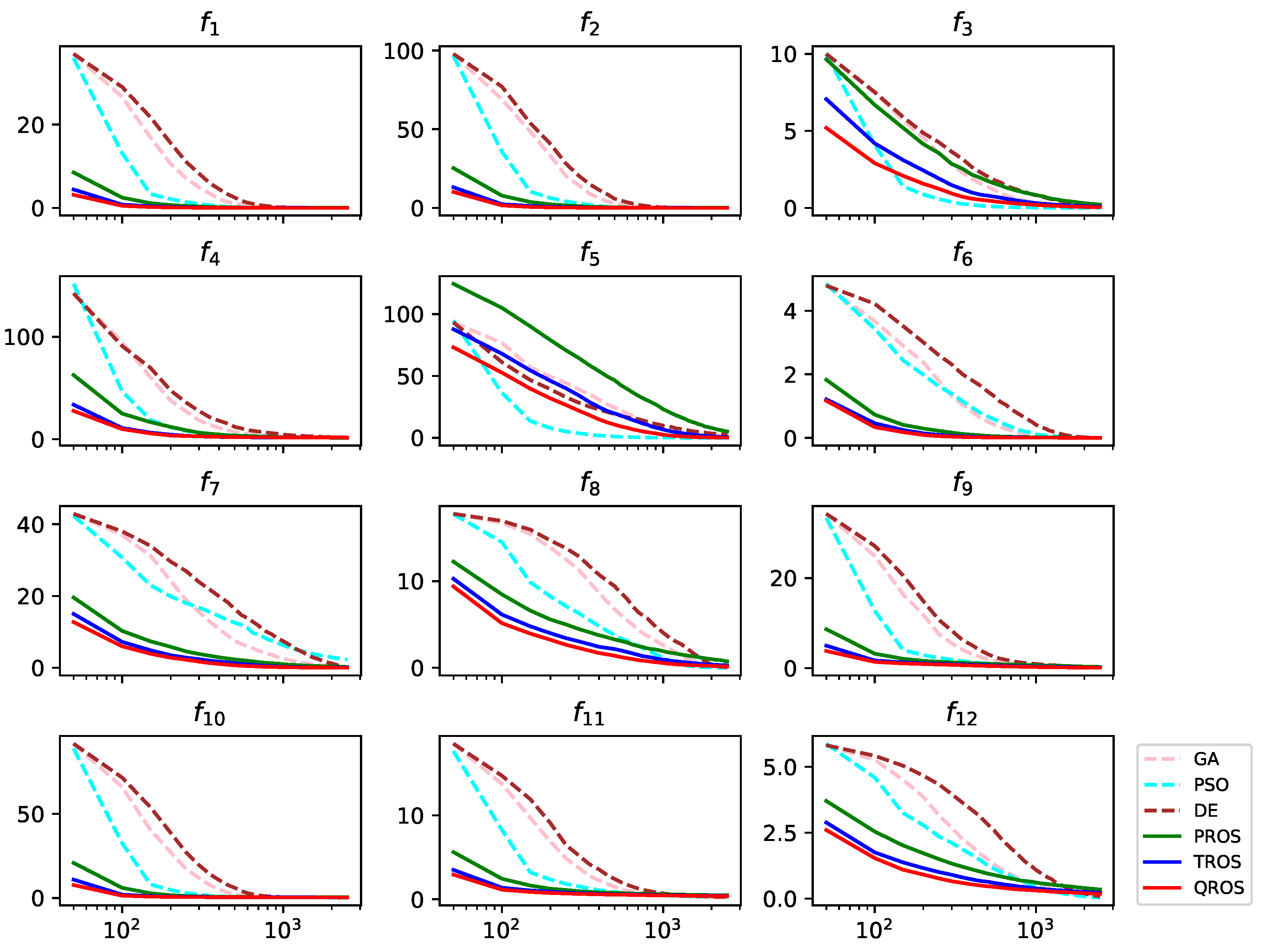
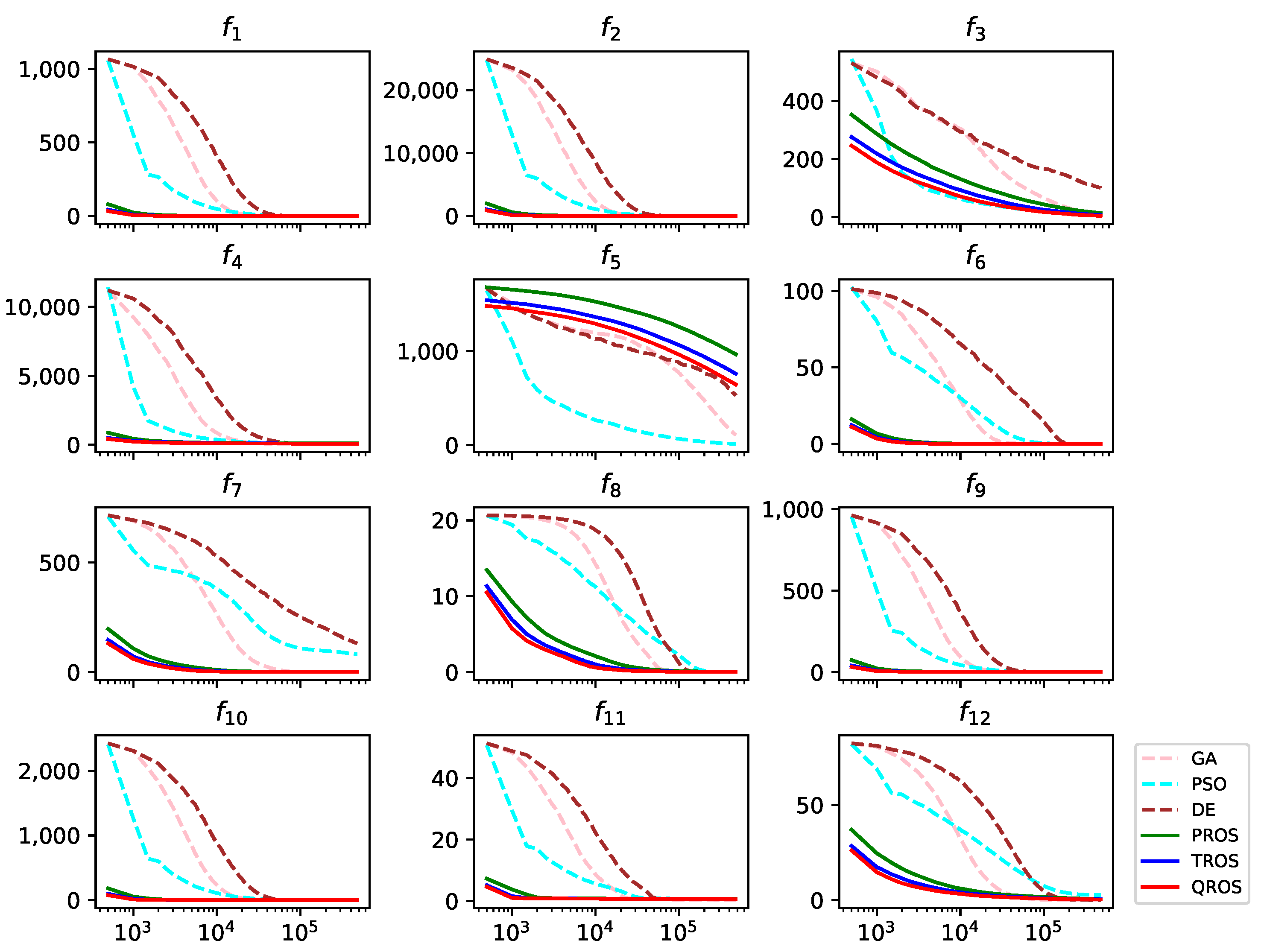
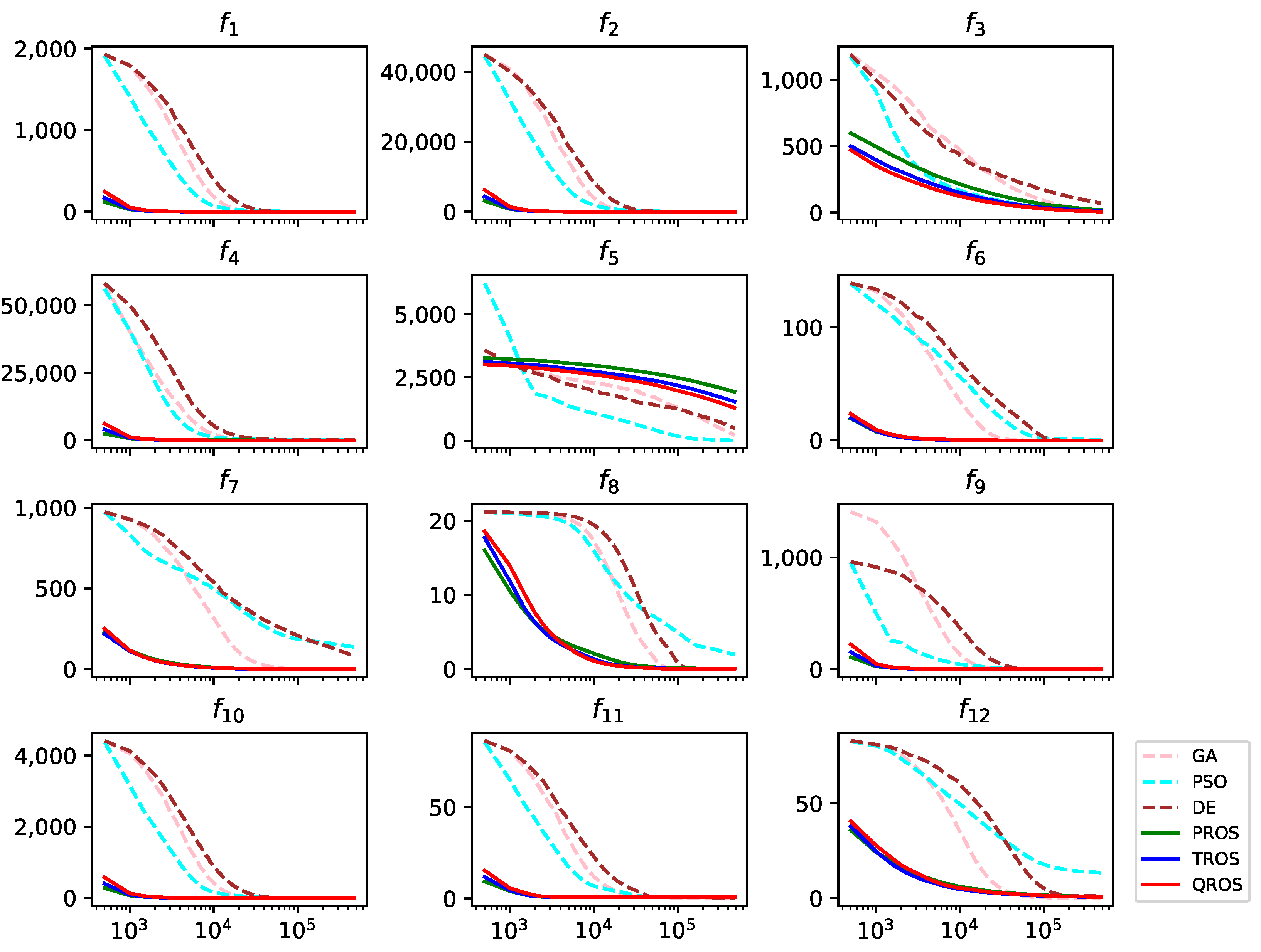
Figure 4 shows the experimental results of the mean error for 100 independent runs of each of the algorithms on each benchmark problem for dimension D = 5 . The x-axes are the number of objective function evaluations (in log scale) and the y-axes are the average error of the algorithm after certain objective function evaluations. As shown in the figure, QROS converged faster than the other five algorithms except on f 3 and f 5 where PSO converged the fastest. TROS and PROS had similar trends as QROS on the benchmark functions: they converged faster than GA, PSO and DE on most benchmark functions except on f 3 and f 5 . Figure 5 and Figure 6 show the experimental results for dimension D = 10 and D = 50 , respectively. Similar to the results for D = 5 , QROS converged faster than the other five algorithms except on f 3 (for 10D) and f 5 (for 10D and 50D) where PSO converged the fastest.
Table 3 shows the mean of the errors of the final solution vectors returned by PROS, TROS and QROS for 100 independent runs of on each benchmark problem for dimension D = 5 . The mean errors represent the medium to long term performance of the algorithms. The best results (the smallest mean final errors) for each benchmark problem are highlighted in bold font. The corresponding standard deviations are placed next with parenthesis. Owing to limited space, the results of GA, PSO and DE are not shown here, as they have been reported in [15] already. As seen from the table, QROS had the smallest mean final errors on most of the benchmark problems. Similar results can be seen from Table 4 and Table 5 which show the means of the final errors for dimension D = 10 and D = 50 , respectively. In general, QROS and TROS are more efficient in reducing the mean final errors on most benchmark problems when compared with PROS.

4.2. Experiment II: Random Shifted Benchmark Problems

One may notice that both TROS and QROS are in favor of objective functions with the global optimum located at the center of the search space. For example, the global optimum of f 1 , f 2 , f 3 , f 5 , f 6 , f 7 , f 8 , f 9 , f 12 is ( 0 , 0 , , 0 ) . In order to test the effectiveness of TROS and QROS in a general case, another experiment was conducted. The same set of benchmark problems were used in this experiment, but the search space was shifted so that the global optimum may be located anywhere within the bounded search space. A random point o = ( o 1 , o 2 , , o D ) is drawn uniformly from Ω = [ a 1 x 1 * , b 1 x 1 * ] × [ a 2 x 2 * , b 2 x 2 * ] × × [ a D x D * , b D x D * ] for each benchmark function for each run where a i , b i , x i * are the lower limit, upper limit and the optimum value of the i-th decision variable in the original search space of the benchmark function being optimized and i { 1 , 2 , , D } . The shifted search space becomes Ω = [ a 1 o 1 , b 1 o 1 ] × [ a 2 o 2 , b 2 o 2 ] × × [ a D o D , b D o D ] . It has to be noted that the benchmark problems are carefully chosen in this experiment to ensure for each benchmark problem, x * is still the global optimum in the shifted search space but x * is not necessarily be located at the center of the new search space.
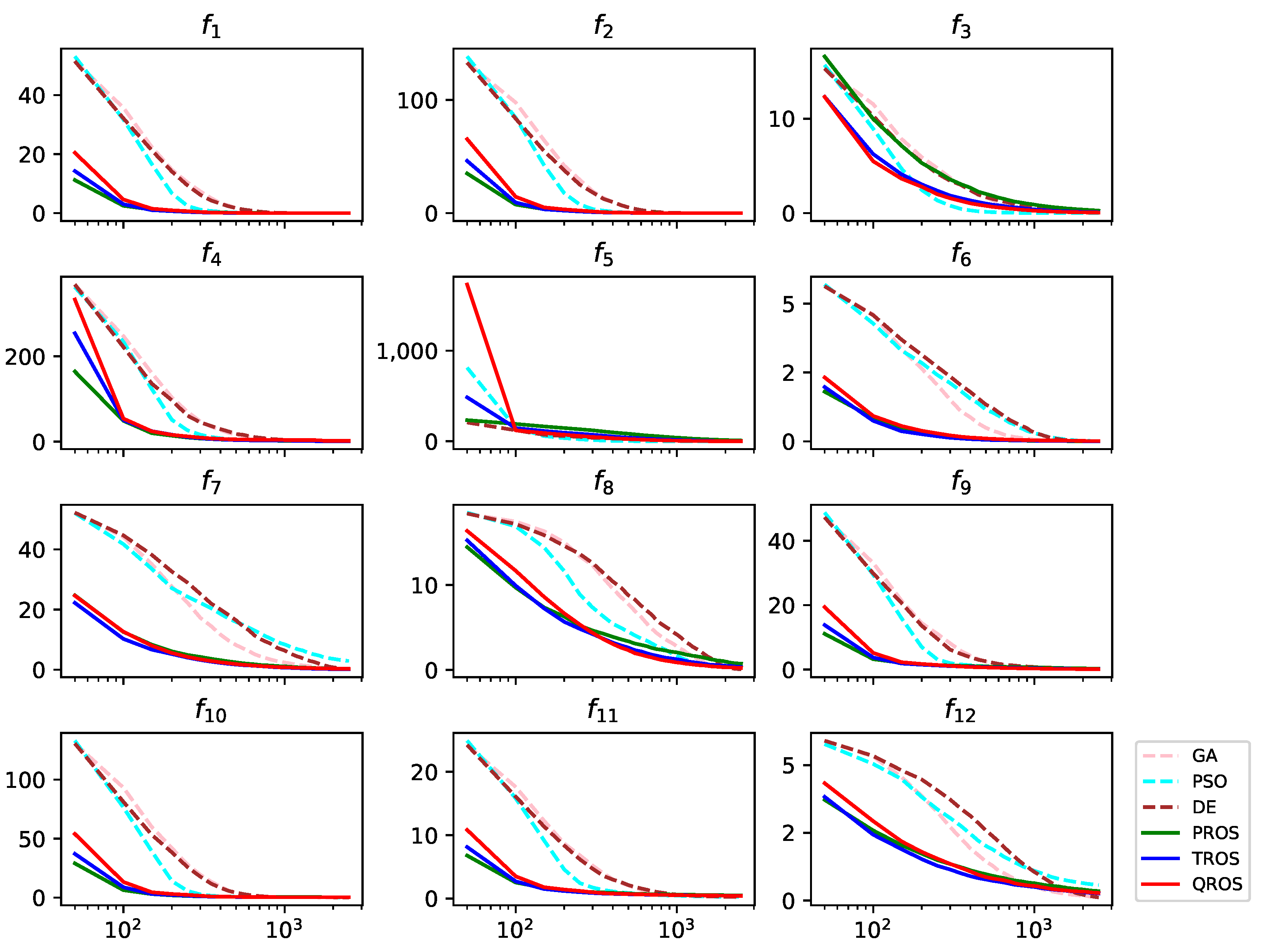
Figure 7, Figure 8 and Figure 9 show the experimental results of the mean error of each of the algorithms on each benchmark problem for dimension D = 5 , D = 10 and D = 50 , respectively. Similar to the non-shifted experiments, PROS, TROS and QROS converged faster than GA, PSO and DE on most benchmark problems except on f 5 when D = 50 . When only considering the three random orthogonal search algorithms, PROS usually converged quickly initially, then TROS surpassed PROS, followed by QROS surpassed TROS on most of the benchmark problems.
Table 6, Table 7 and Table 8 show the statistical results of the final error of each of the algorithms on each benchmark problem for dimension D = 5 , D = 10 and D = 50 , respectively. Similar to the non-shifted experiments, both QROS and TROS often improve the mean final errors. The performance of QROS and TROS are quite promising on the shifted benchmark functions.

5. Future Work

In our future work, we plan to extend the algorithms in two directions. The first one is to allow switching between various sampling polices (e.g., uniform, triangular, quadratic) in an adaptive way. This is particular useful for black-box optimization where the form of the function is unknown to the optimization algorithm. One could learn the best sampling policy for that particular function and adapt gradually from the results of previous function evaluations. The second direction is to gradually rotate the objective function based on the current best solution set [22,23]. By doing so, a complex function would be transformed to a simpler convex function in the small area of concern. Any simple techniques such as TROS and QROS would quickly converge to the global optimum if it is in the area of concern. We are interested in investigating the convergence of TROS and QROS with the addition of transformation techniques.

6. Conclusions

In this paper, we perform an analysis of PROS. PROS is a parameterless EA that outperforms several well-known optimization algorithms on benchmark functions when the search budget is limited. It is attractive for expensive optimizing problems. However, to the best of our knowledge, there is no mathematical analysis of the performance and behavior of PROS reported in the literature. In this paper, we fill this gap.
Moreover, we propose TROS and QROS, which preserve the advantages of PROS and outperform it. We perform an analysis of t a m e convergence for PROS, TROS and QROS. We conduct two sets of experiments to evaluate the performance of TROS and QROS. We increase the number of runs compared to those conducted in [15] in order to increase the reliability of the statistical results. Experimental results illustrate that TROS and QROS outperform PROS to a large extent. Both TROS and QROS converge quickly on the benchmark problems. Although GA, PSO and DE usually have better performance in terms of smaller error in the final solution when a considerable amount of objective function evaluation is given, the performances of QROS and TROS are not much inferior to that of GA, PSO and DE. In fact, QROS and TROS are even sensible choices when we consider the computational complexity.

Author Contributions

Conceptualization, B.K.-B.T., C.W.S. and W.S.W.; methodology, B.K.-B.T. and W.S.W.; software, B.K.-B.T.; validation, B.K.-B.T.; formal analysis, B.K.-B.T., C.W.S. and W.S.W.; investigation, B.K.-B.T.; resources, B.K.-B.T.; data curation, B.K.-B.T.; writing—original draft preparation, B.K.-B.T.; writing—review and editing, B.K.-B.T., C.W.S. and W.S.W.; visualization, B.K.-B.T.; supervision, W.S.W.; project adminstration, B.K.-B.T.; funding acquisition, B.K.-B.T. All authors have read and agreed to the published version of the manuscript.

Funding

The APC was partially funded by Hong Kong Metropolitan University.

Institutional Review Board Statement

Not applicable.

Informed Consent Statement

Not applicable.

Data Availability Statement

Data are available from the authors upon reasonable request.

Conflicts of Interest

The authors declare no conflict of interest.

References

  1. Cao, Y.; Zhang, H.; Li, W.; Zhou, M.; Zhang, Y.; Chaovalitwongse, W.A. Comprehensive Learning Particle Swarm Optimization Algorithm With Local Search for Multimodal Functions. IEEE Trans. Evol. Comput. 2019, 23, 718–731. [Google Scholar] [CrossRef]
  2. Kang, Q.; Song, X.; Zhou, M.; Li, L. A Collaborative Resource Allocation Strategy for Decomposition-Based Multiobjective Evolutionary Algorithms. IEEE Trans. Syst. Man Cybern. Syst. 2019, 49, 2416–2423. [Google Scholar] [CrossRef]
  3. Liu, J.; Liu, Y.; Jin, Y.; Li, F. A Decision Variable Assortment-Based Evolutionary Algorithm for Dominance Robust Multiobjective Optimization. IEEE Trans. Syst. Man Cybern. Syst. 2022, 52, 3360–3375. [Google Scholar] [CrossRef]
  4. Sarker, R.A.; Kamruzzaman, J.; Newton, C.S. Evolutionary Optimization (Evopt): A Brief Review And Analysis. Int. J. Comput. Intell. Appl. 2003, 3, 311–330. [Google Scholar] [CrossRef]
  5. Tian, J.; Tan, Y.; Zeng, J.; Sun, C.; Jin, Y. Multiobjective Infill Criterion Driven Gaussian Process-Assisted Particle Swarm Optimization of High-Dimensional Expensive Problems. IEEE Trans. Evol. Comput. 2019, 23, 459–472. [Google Scholar] [CrossRef]
  6. Jin, Y.; Wang, H.; Chugh, T.; Guo, D.; Miettinen, K. Data-Driven Evolutionary Optimization: An Overview and Case Studies. IEEE Trans. Evol. Comput. 2019, 23, 442–458. [Google Scholar] [CrossRef]
  7. Yang, C.; Ding, J.; Jin, Y.; Chai, T. Offline Data-Driven Multiobjective Optimization: Knowledge Transfer Between Surrogates and Generation of Final Solutions. IEEE Trans. Evol. Comput. 2020, 24, 409–423. [Google Scholar] [CrossRef] [Green Version]
  8. Liu, Y.; Liu, J.; Jin, Y. Surrogate-Assisted Multipopulation Particle Swarm Optimizer for High-Dimensional Expensive Optimization. IEEE Trans. Syst. Man Cybern. Syst. 2022, 52, 4671–4684. [Google Scholar] [CrossRef]
  9. Zhou, Y.; He, X.; Chen, Z.; Jiang, S. A Neighborhood Regression Optimization Algorithm for Computationally Expensive Optimization Problems. IEEE Trans. Cybern. 2022, 52, 3018–3031. [Google Scholar] [CrossRef] [PubMed]
  10. Gutjahr, W.J. Convergence Analysis of Metaheuristics. In Matheuristics: Hybridizing Metaheuristics and Mathematical Programming; Maniezzo, V., Stützle, T., Voß, S., Eds.; Springer: Boston, MA, USA, 2010; pp. 159–187. [Google Scholar] [CrossRef]
  11. Zamani, S.; Hemmati, H. A Cost-Effective Approach for Hyper-Parameter Tuning in Search-based Test Case Generation. In Proceedings of the 2020 IEEE International Conference on Software Maintenance and Evolution (ICSME), Adelaide, Australia, 28 September–2 October 2020; pp. 418–429. [Google Scholar] [CrossRef]
  12. Gu, Q.; Wang, Q.; Xiong, N.N.; Jiang, S.; Chen, L. Surrogate-assisted Evolutionary Algorithm for Expensive Constrained Multi-objective Discrete Optimization Problems. Complex Intell. Syst. 2022, 8, 2699–2718. [Google Scholar] [CrossRef]
  13. Sarker, R.A.; Elsayed, S.M.; Ray, T. Differential Evolution With Dynamic Parameters Selection for Optimization Problems. IEEE Trans. Evol. Comput. 2014, 18, 689–707. [Google Scholar] [CrossRef]
  14. Karafotias, G.; Hoogendoorn, M.; Eiben, A.E. Parameter Control in Evolutionary Algorithms: Trends and Challenges. IEEE Trans. Evol. Comput. 2015, 19, 167–187. [Google Scholar] [CrossRef]
  15. Plevris, V.; Bakas, N.P.; Solorzano, G. Pure Random Orthogonal Search (PROS): A Plain and Elegant Parameterless Algorithm for Global Optimization. Appl. Sci. 2021, 11, 5053. [Google Scholar] [CrossRef]
  16. Vesterstrom, J.; Thomsen, R. A Comparative Study of Differential Evolution, Particle Swarm Optimization, and Evolutionary Algorithms on Numerical Benchmark Problems. In Proceedings of the 2004 Congress on Evolutionary Computation (IEEE Cat. No.04TH8753), Portland, OR, USA, 19–23 June 2004; Volume 2, pp. 1980–1987. [Google Scholar] [CrossRef]
  17. Omidvar, M.N.; Li, X.; Tang, K. Designing Benchmark Problems for Large-scale Continuous Optimization. Inf. Sci. 2015, 316, 419–436. [Google Scholar] [CrossRef]
  18. Holland, J.H. Adaptation in Natural and Artificial Systems; The University of Michigan Press: Ann Arbor, MI, USA, 1975. [Google Scholar]
  19. Kennedy, J.; Eberhart, R. Particle Swarm Optimization. In Proceedings of the ICNN’95—International Conference on Neural Networks, Perth, Australia, 27 November–1 December 1995; Volume 4, pp. 1942–1948. [Google Scholar] [CrossRef]
  20. Storn, R.; Price, K. Differential Evolution—A Simple and Efficient Heuristic for global Optimization over Continuous Spaces. J. Glob. Optim. 1997, 11, 341–359. [Google Scholar] [CrossRef]
  21. Blank, J.; Deb, K. Pymoo: Multi-Objective Optimization in Python. IEEE Access 2020, 8, 89497–89509. [Google Scholar] [CrossRef]
  22. Hansen, N. Adaptive Encoding: How to Render Search Coordinate System Invariant. In Parallel Problem Solving from Nature—PPSN X; Rudolph, G., Jansen, T., Beume, N., Lucas, S., Poloni, C., Eds.; Springer: Berlin/Heidelberg, Germany, 2008; pp. 205–214. [Google Scholar] [CrossRef] [Green Version]
  23. Loshchilov, I.; Schoenauer, M.; Sebag, M. Adaptive Coordinate Descent. In Proceedings of the 13th Annual Conference on Genetic and Evolutionary Computation, GECCO ’11, Dublin, Ireland, 12–16 July 2011; pp. 885–892. [Google Scholar] [CrossRef]
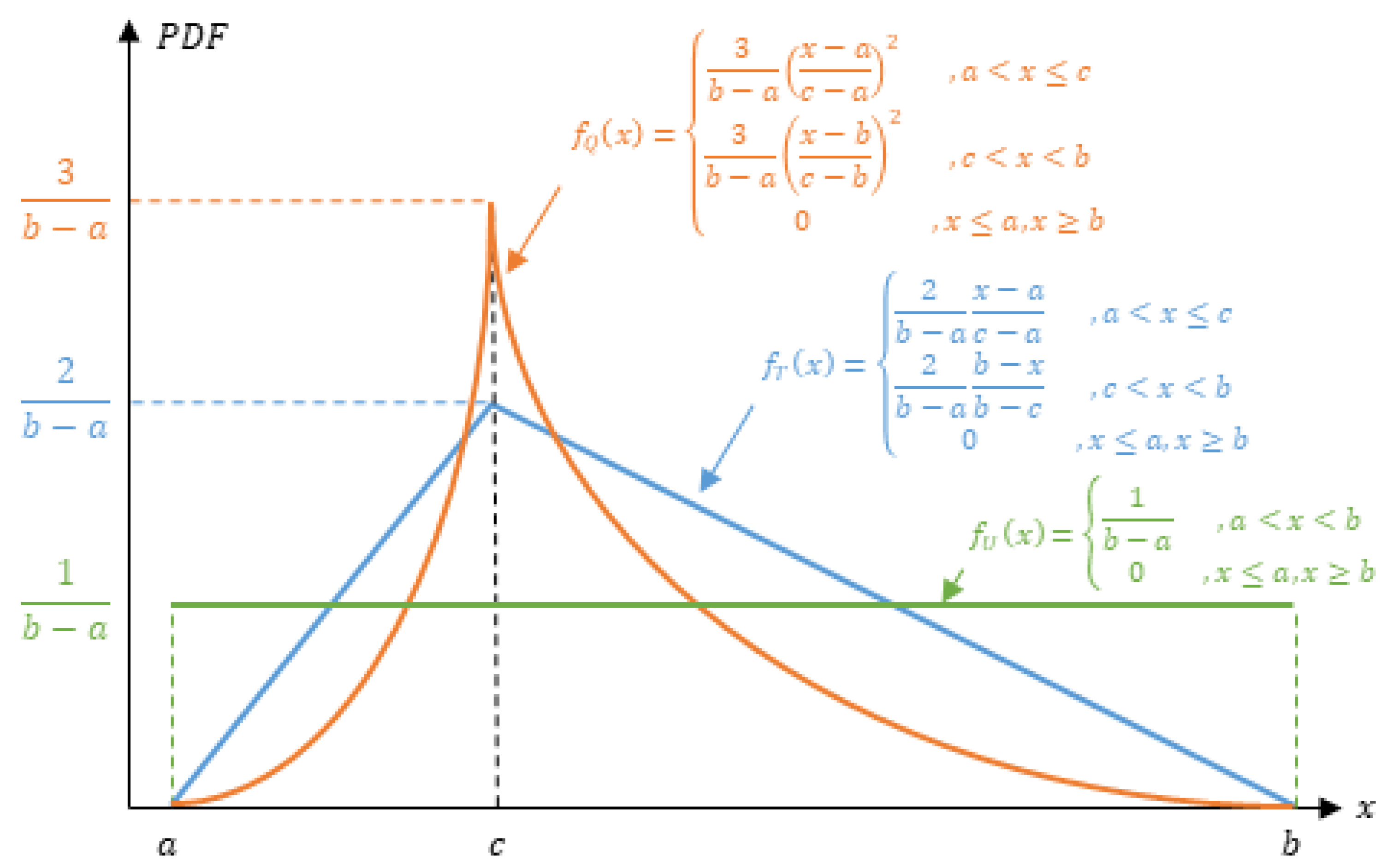
Figure 1. The probability density function of the triangular distribution T ( a , b , c ) , the quadratic distribution Q ( a , b , c ) , and uniform distribution U ( a , b ) .
Applsci 13 01391 g001
Figure 2. Left: an example function where x ( t ) < x j * . Right: another example function where x ( t ) > x j * . The set of t a m e solutions is denoted as S j .
Applsci 13 01391 g002
Figure 3. An example convex function. Left: for case 1, x j ( t ) < x j * , u j = 0 . Right: case 2, x j ( t ) > x j * , r j = 0 .
Applsci 13 01391 g003
Figure 4. The convergence curve of 100 runs on 5D benchmark functions.
Applsci 13 01391 g004
Figure 5. The convergence curve of 100 runs on 10D benchmark functions.
Applsci 13 01391 g005
Figure 6. The convergence curve of 30 runs on 50D benchmark functions.
Applsci 13 01391 g006
Figure 7. The convergence curve of 100 runs on 5D benchmark functions with shifted global optimum.
Applsci 13 01391 g007
Figure 8. The convergence curve of 100 runs on 10D benchmark functions with shifted global optimum.
Applsci 13 01391 g008
Figure 9. The convergence curve of 30 runs on 50D benchmark functions with shifted global optimum.
Applsci 13 01391 g009
Table 1. Benchmark test problems. (Unimodal functions: f 1 f 5 ; multimodal functions: f 6 f 12 ; convex functions: f 1 f 2 , f 5 ; non-convex functions: f 3 f 4 , f 6 f 12 ; separable functions: f 1 f 2 , f 6 f 7 , f 12 ; non-separable functions: f 3 f 5 , f 8 f 11 ).
No.FunctionFormulation and Global OptimumSearch Space
f 1 Sphere i = 1 D x i 2 [ 10 , 10 ] D
x * = ( 0 , 0 , , 0 ) , f ( x * ) = 0
f 2 Ellipsoid i = 1 D i x i 2 [ 10 , 10 ] D
x * = ( 0 , 0 , , 0 ) , f ( x * ) = 0
f 3 Schwefel 1.2 i = 1 D ( j = 1 i x j ) 2 [ 5.12 , 5.12 ] D
x * = ( 0 , 0 , , 0 ) , f ( x * ) = 0
f 4 Rosenbrock i = 1 D 1 [ 100 ( x i + 1 x i 2 ) 2 + ( x i 1 ) 2 ] [ 2.048 , 2.048 ] D
x * = ( 1 , 1 , , 1 ) , f ( x * ) = 0
f 5 Zakharov i = 1 D x i 2 + ( 1 2 i = 1 D i x i ) 2 + ( 1 2 i = 1 D i x i ) 4 [ 10 , 10 ] D
x * = ( 0 , 0 , , 0 ) , f ( x * ) = 0
f 6 Alpine 1 i = 1 D | x i sin ( x i ) + 0.1 x i | [ 10 , 10 ] D
x * = ( 0 , 0 , , 0 ) , f ( x * ) = 0
f 7 Rastrigin 10 D + i = 1 D [ x i 2 10 cos ( 2 π x i ) ] [ 5.12 , 5.12 ] D
x * = ( 0 , 0 , , 0 ) , f ( x * ) = 0
f 8 Ackley 20 + exp ( 1 ) 20 exp ( 0.2 1 D i = 1 D x i 2 ) [ 32.768 , 32.768 ] D
exp ( 1 D i = 1 D cos ( 2 π x i ) )
x * = ( 0 , 0 , , 0 ) , f ( x * ) = 0
f 9 Griewank i = 1 D x i 2 4000 i = 1 D cos ( x i i ) + 1 [ 600 , 600 ] D
x * = ( 0 , 0 , , 0 ) , f ( x * ) = 0
f 10 HGBat | ( i = 1 D x i 2 ) 2 ( i = 1 D x i ) 2 | 1 / 2 + [ 15 , 15 ] D
( 0.5 i = 1 D x i 2 + i = 1 D x i ) / D + 0.5
x * = ( 1 , 1 , , 1 ) , f ( x * ) = 0
f 11 HappyCat | i = 1 D x i 2 D | 1 / 4 + [ 20 , 20 ] D
( 0.5 i = 1 D x i 2 + i = 1 D x i ) / D + 0.5
x * = ( 1 , 1 , , 1 ) , f ( x * ) = 0
f 12 Weierstrass i = 1 D [ k = 0 20 0.5 k cos ( 2 π 3 k ( x i + 0.5 ) ) [ 0.5 , 0.5 ] D
D k = 0 20 0.5 k cos ( π 3 k ) ]
x * = ( 0 , 0 , , 0 ) , f ( x * ) = 0
Table 2. Settings of the numerical experiments.
Settings D = 5 D = 10 D = 50
Population Size 10 D 50100500
Max. No. of Generations ( 20 D 50 ) 50150950
Max. No. of Objective 10 D ( 20 D 50 ) 250015,000475,000
Function Evaluations
No. of Runs 10010030
Table 3. Statistical results of 100 runs on 5D benchmark functions.
fPROSTROSQROS
f 1 4.65e-03 (4.85e-03)1.06e-03 (8.88e-04)4.13e-04 (4.54e-04)
f 2 1.38e-02 (1.68e-02)3.13e-03 (2.65e-03)1.21e-03 (1.33e-03)
f 3 2.17e-01 (1.80e-01)7.61e-02 (5.05e-02)4.32e-02 (2.99e-02)
f 4 1.34e+00 (1.17e+00)1.48e+00 (1.16e+00)1.55e+00 (1.17e+00)
f 5 5.13e+00 (6.46e+00)5.33e-01 (8.45e-01)1.28e-01 (1.81e-01)
f 6 4.81e-03 (3.68e-03)2.38e-03 (9.69e-04)1.62e-03 (7.19e-04)
f 7 2.41e-01 (2.49e-01)5.30e-02 (4.49e-02)2.91e-02 (3.01e-02)
f 8 7.48e-01 (4.80e-01)2.81e-01 (1.65e-01)1.53e-01 (8.95e-02)
f 9 2.69e-01 (1.41e-01)1.33e-01 (6.76e-02)8.98e-02 (3.69e-02)
f 10 4.01e-01 (1.40e-01)3.34e-01 (1.24e-01)2.83e-01 (1.26e-01)
f 11 4.67e-01 (1.34e-01)4.05e-01 (1.20e-01)3.72e-01 (9.48e-02)
f 12 3.49e-01 (1.04e-01)2.22e-01 (6.44e-02)1.77e-01 (4.67e-02)
Table 4. Statistical results of 100 runs on 10D benchmark functions.
fPROSTROSQROS
f 1 8.62e-04 (7.26e-04)2.38e-04 (1.85e-04)1.03e-04 (7.51e-05)
f 2 4.45e-03 (3.33e-03)1.34e-03 (1.23e-03)5.68e-04 (4.63e-04)
f 3 6.84e-01 (3.62e-01)2.52e-01 (1.35e-01)1.35e-01 (7.28e-02)
f 4 3.40e+00 (3.28e+00)3.72e+00 (2.99e+00)4.53e+00 (2.91e+00)
f 5 4.69e+01 (2.47e+01)1.40e+01 (9.29e+00)6.26e+00 (4.77e+00)
f 6 3.10e-03 (9.52e-04)1.70e-03 (5.30e-04)1.10e-03 (3.52e-04)
f 7 4.48e-02 (3.77e-02)1.24e-02 (9.46e-03)5.24e-03 (3.56e-03)
f 8 1.61e-01 (8.23e-02)7.13e-02 (3.00e-02)4.32e-02 (1.55e-02)
f 9 1.78e-01 (6.53e-02)9.15e-02 (3.68e-02)6.77e-02 (2.74e-02)
f 10 4.73e-01 (2.46e-01)4.35e-01 (1.97e-01)4.31e-01 (1.99e-01)
f 11 4.90e-01 (1.65e-01)4.30e-01 (1.49e-01)3.76e-01 (1.17e-01)
f 12 3.40e-01 (8.16e-02)2.20e-01 (4.97e-02)1.68e-01 (3.85e-02)
Table 5. Statistical results of 30 runs on 50D benchmark functions.
fPROSTROSQROS
f 1 1.12e-04 (3.30e-05)2.82e-05 (7.60e-06)1.24e-05 (4.68e-06)
f 2 2.86e-03 (9.68e-04)7.25e-04 (2.22e-04)3.29e-04 (1.32e-04)
f 3 1.34e+01 (3.13e+00)6.45e+00 (1.57e+00)3.75e+00 (8.21e-01)
f 4 8.06e+01 (3.80e+01)6.05e+01 (3.41e+01)5.48e+01 (2.46e+01)
f 5 9.66e+02 (1.63e+02)7.58e+02 (1.51e+02)6.44e+02 (1.36e+02)
f 6 2.46e-03 (3.48e-04)1.32e-03 (1.93e-04)8.85e-04 (1.26e-04)
f 7 5.81e-03 (1.72e-03)1.32e-03 (2.79e-04)6.25e-04 (1.60e-04)
f 8 2.06e-02 (3.28e-03)9.90e-03 (1.13e-03)6.49e-03 (9.52e-04)
f 9 2.63e-02 (1.51e-02)1.17e-02 (1.01e-02)1.39e-02 (1.77e-02)
f 10 5.99e-01 (2.48e-01)5.80e-01 (2.25e-01)5.66e-01 (2.27e-01)
f 11 6.51e-01 (1.28e-01)6.17e-01 (1.11e-01)6.21e-01 (1.08e-01)
f 12 5.34e-01 (4.80e-02)3.43e-01 (2.93e-02)2.61e-01 (2.84e-02)
Table 6. Statistical results of 100 runs on 5D benchmark functions with shifted global optimum.
fPROSTROSQROS
f 1 4.31e-03 (4.38e-03)1.67e-03 (3.92e-03)1.15e-03 (5.90e-03)
f 2 1.24e-02 (1.20e-02)4.41e-03 (7.05e-03)2.60e-03 (9.36e-03)
f 3 2.64e-01 (2.23e-01)9.43e-02 (8.36e-02)5.54e-02 (4.39e-02)
f 4 1.38e+00 (3.51e+00)9.47e-01 (3.44e+00)1.82e+00 (1.12e+01)
f 5 7.76e+00 (1.24e+01)8.39e-01 (1.16e+00)2.60e-01 (4.88e-01)
f 6 4.62e-03 (2.28e-03)6.57e-03 (9.53e-03)1.21e-02 (1.96e-02)
f 7 2.23e-01 (2.23e-01)1.39e-01 (3.07e-01)2.97e-01 (5.00e-01)
f 8 7.34e-01 (4.52e-01)3.27e-01 (2.86e-01)2.34e-01 (3.01e-01)
f 9 2.94e-01 (1.97e-01)1.54e-01 (7.26e-02)1.18e-01 (1.06e-01)
f 10 3.90e-01 (1.68e-01)3.18e-01 (1.22e-01)3.13e-01 (1.38e-01)
f 11 4.82e-01 (1.21e-01)4.28e-01 (1.43e-01)4.15e-01 (1.93e-01)
f 12 3.47e-01 (1.03e-01)2.64e-01 (1.33e-01)2.79e-01 (2.32e-01)
Table 7. Statistical results of 100 runs on 10D benchmark functions with shifted global optimum.
fPROSTROSQROS
f 1 8.71e-04 (5.89e-04)2.55e-04 (1.99e-04)1.64e-04 (2.97e-04)
f 2 4.64e-03 (3.58e-03)1.33e-03 (1.18e-03)9.91e-04 (2.60e-03)
f 3 7.99e-01 (4.64e-01)2.78e-01 (1.76e-01)1.62e-01 (9.67e-02)
f 4 1.35e+00 (6.26e+00)8.60e-01 (2.81e+00)8.20e-01 (2.68e+00)
f 5 6.23e+01 (4.86e+01)1.80e+01 (1.70e+01)7.34e+00 (7.04e+00)
f 6 3.12e-03 (9.80e-04)2.38e-03 (2.74e-03)6.05e-03 (9.72e-03)
f 7 4.53e-02 (3.06e-02)6.38e-02 (2.58e-01)2.65e-01 (5.19e-01)
f 8 1.64e-01 (7.02e-02)8.10e-02 (3.39e-02)6.33e-02 (1.06e-01)
f 9 1.85e-01 (6.35e-02)9.56e-02 (3.76e-02)7.97e-02 (3.49e-02)
f 10 3.84e-01 (2.06e-01)3.61e-01 (1.80e-01)3.37e-01 (1.96e-01)
f 11 4.50e-01 (1.46e-01)4.51e-01 (2.05e-01)4.45e-01 (1.92e-01)
f 12 3.31e-01 (7.39e-02)2.52e-01 (9.44e-02)3.03e-01 (2.26e-01)
Table 8. Statistical results of 30 runs on 50D benchmark functions with shifted global optimum.
fPROSTROSQROS
f 1 1.13e-04 (2.63e-05)2.88e-05 (1.00e-05)1.30e-05 (4.43e-06)
f 2 2.90e-03 (7.79e-04)7.43e-04 (3.28e-04)3.31e-04 (1.23e-04)
f 3 1.78e+01 (4.20e+00)8.55e+00 (1.75e+00)5.46e+00 (1.20e+00)
f 4 2.02e+01 (3.98e+01)2.59e+00 (8.90e+00)3.84e+00 (1.35e+01)
f 5 1.93e+03 (4.23e+02)1.55e+03 (3.24e+02)1.30e+03 (2.85e+02)
f 6 2.62e-03 (3.48e-04)1.69e-03 (5.51e-04)3.19e-03 (2.83e-03)
f 7 5.89e-03 (1.37e-03)1.58e-03 (4.07e-04)2.99e-01 (5.23e-01)
f 8 2.09e-02 (2.66e-03)9.85e-03 (1.31e-03)6.68e-03 (1.06e-03)
f 9 2.77e-02 (1.27e-02)1.92e-02 (1.70e-02)5.13e-02 (4.70e-02)
f 10 3.68e-01 (1.11e-01)3.70e-01 (1.55e-01)3.32e-01 (9.46e-02)
f 11 5.82e-01 (1.11e-01)5.74e-01 (9.44e-02)6.06e-01 (1.34e-01)
f 12 5.51e-01 (4.15e-02)3.93e-01 (1.21e-01)5.14e-01 (2.79e-01)
Disclaimer/Publisher’s Note: The statements, opinions and data contained in all publications are solely those of the individual author(s) and contributor(s) and not of MDPI and/or the editor(s). MDPI and/or the editor(s) disclaim responsibility for any injury to people or property resulting from any ideas, methods, instructions or products referred to in the content.