Article

Optimization on Linkage System for Vehicle Wipers by the Method of Differential Evolution

1
Department of Vehicle Engineering, National Pingtung University of Science and Technology, Pingtung 912, Taiwan
2
Department of Mathematics, National Cheng-Kung University, Tainan City 701, Taiwan
*
Author to whom correspondence should be addressed.
Appl. Sci. 2023, 13(1), 332; https://doi.org/10.3390/app13010332
Submission received: 30 November 2022 / Revised: 19 December 2022 / Accepted: 23 December 2022 / Published: 27 December 2022
(This article belongs to the Special Issue Evolutionary Computation: Theories, Techniques, and Applications)

Abstract

:
We consider an optimization problem on the maximal magnitude of angular acceleration of the output-links of a commercially available center-driven linkage system (CDLS) for vehicle wipers on windshield. The purpose of this optimization is to improve the steadiness of a linkage system without weakening its normal function. Thus this optimization problem is considered under the assumptions that the frame of the fixed links of linkage system is unchanged and that the input-link rotates at the same constant angular speed with its length unchanged. To meet the usual requirements for vehicle wipers on windshield, this optimization problem must be solved subject to 10 specific constraints. We expect that optimizing the maximal magnitude of angular acceleration of the output-links of a linkage system would also be helpful for reducing the amplitudes of sound waves of wiper noise. We establish the motion model of CDLS and then justify this model with ADAMS. We use a “Differential Evolution” type method to search for the minimum of an objective function subject to 10 constraints for this optimization problem. Our optimization computation shows that the maximal magnitude of angular acceleration of both output-links of this linkage system can be reduced by more than 10%.

1. Introduction

Linkage systems are widely used on vehicles. Research on the design of linkage systems is important for vehicle industry development. In this article, we consider the linkage systems for vehicle wipers. Our goal is to improve the steadiness of a linkage system for vehicle wipers without weakening its normal function. This improvement on the steadiness of a linkage system for vehicle wipers could reduce the possible material fatigue of a linkage system. Besides, this improvement could also be helpful for reducing the unpleasant rubber wiper noise on vehicle windshield.
The linkage systems considered in this article are the center driven linkage systems (CDLS). A center driven linkage system is a composition of two crank-rocker linkage systems driven by a single central input-link. A crank-rocker linkage system is shown in the following Figure 1.
In Figure 1, the link OB is a fixed link with length q . The link OA, with length s , may rotates full 360 degrees and is called the “crank” of this linkage system. Usually the crank is driven by a motor. The link BC, with length p , may only moves on a limited circular sector and is called the “rocker” of this linkage system. The link AC usually has the longest length l and acts as the transfer link of this linkage system. Generally the Grashof law
s + l < p + q
for crank-rocker system must be satisfied. See [1] for more discussions on linkage systems.
To improve the steadiness of a linkage system without weakening its normal function, we will consider an optimization problem on the maximal magnitude of angular acceleration of the output-links of a CDLS under the assumptions that the frame of the fixed links of linkage system is unchanged and that the input link rotates at the same (constant) angular speed with its length unchanged. To meet the usual requirements for vehicle wipers on windshield, this optimization problem must be solved subject to 10 specific constraints.
To tackle this optimization problem, we will use a Differential Evolution type search method. The usual stages of a DE search algorithm is shown in the following Figure 2.
The method of Differential Evolution (DE) was introduced by Storn and Price in 1995 [2,3,4]. In this DE search method, two important parameters F (the scale factor) and C R (the crossover ratio), for the mutation and crossover operations of DE, can be selected respectively from the interval [ 0 , 1 ] . These parameters are important both for controlling the diversity of “generation population” and for controlling the convergence rate of DE.
The space complexity of DE is usually relatively low, when compared with the highly efficient “restart covariance matrix adaptation evolution strategies (restart CMA-ES)”. Besides, the control parameters F (the scale factor) and C R (the crossover ratio) can be adjusted to improve the performance of the DE algorithm easily without causing serious computational burden. Moreover, the introduction of mutation operator by “difference vectors” in DE obviously speed up the computational convergence of DE.
Because of its simplicity and its experimental efficiency, this DE search method soon has become very popular. Since then, various variants of DE were presented. For examples, there are DE using “Trigonometric Mutation” [5]; “opposition-based learning” DE [6,7,8,9]; DEGL with Neighborhood-Based Mutation [10]; SADE (DE with parameters adjusted through self-adaptive learning) [11,12,13,14]. See [15,16,17] for more information on the various variants of DE.
Though various complicated types of DE methods were presented, research articles on the theoretical analysis of DE are rare. Most of the variants of DE mentioned above were presented only with experimental studies. For classical DE algorithms, “weak convergence” for most objective functions were proved under reasonable assumptions in [18,19,20]. The theoretical analysis of the DE search methods in [18,19,20] provides the foundation for the convergence of the DE type search method adopted in this article.
Our objective function for this optimization problem is defined to be the sum of the maximal absolute values of angular acceleration of the output-links of this linkage system:
f ( r 3 , r 4 , r 5 , r 6 ) = max 0 θ 2 2 π | α 4 ( r 3 , r 4 , θ 2 ) | + max 0 θ 2 2 π | α 6 ( r 5 , r 6 , θ 2 ) | .
This optimization problem must be solved subject to 10 specific constraints. These constraints are from the usual requirements for vehicle wipers on windshield. This objective function is a function of the connecting-links and the output-links respectively on the driver side and on the passenger side of CDLS. Details of this objective function will be discussed in Section 2.
We assume that the input link of this CDLS rotates at a constant speed with angular velocity of 1 rad/s. Our optimization computation for this linkage system shows that the maximal magnitude of the angular acceleration of the output-link on the driver side of this CDLS can be reduced by 10.69%. Besides, our optimization computation for this linkage system shows that the maximal magnitude of the angular acceleration of the output-link on the passenger side of this CDLS can be reduced by 12.10%. Interestingly, our algorithm takes only 30 seconds to finish its searching process for the minimum of the objective function for this optimization problem subject to 10 specific constraints.
This improvement on the steadiness of a linkage system for vehicle wipers is related to our earlier work [21] on the vibration frequencies of rubber wiper on convex windshield. We expect that improvement on the steadiness of a linkage system for vehicle wipers would be helpful for reducing the amplitudes of sound waves of wiper noise around each reversal of the motion of rubber wipers on windshield.
Optimization problems on the “expectation output function” of a linkage system were considered before by some people using Genetic Algorithms on MATLAB. See, for example [22].

2. Materials and Methods

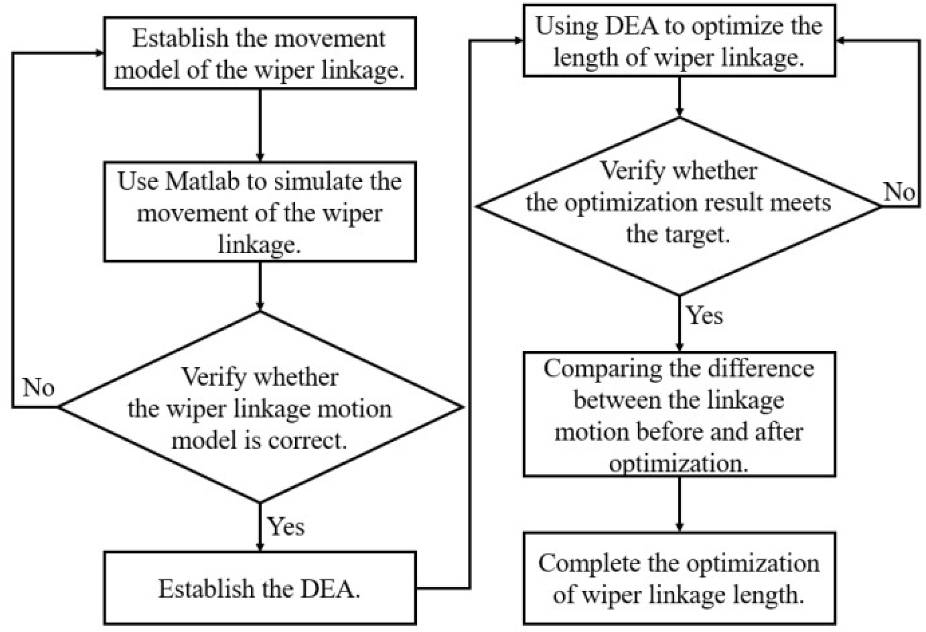
A flowchart of our method is shown in Figure 3. In this section, we will discuss a kinematic model of CDLS. On the basis of this model, mathematical formulas for the angles, the angular velocities, the values of angular acceleration, and the transmission angle of various parts of a CDLS will be established. Numerical simulations of the motion of a CDLS will be performed on MATLAB based on these mathematical formulas. The objective function is defined as follows:
f ( r 3 , r 4 , r 5 , r 6 ) = max 0 θ 2 2 π | α 4 ( r 3 , r 4 , θ 2 ) | + max 0 θ 2 2 π | α 6 ( r 5 , r 6 , θ 2 ) |
in which α 4 and α 6 are the values of angular acceleration of the output-links respectively on the driver side and on the passenger side of a CDLS. We will discuss the mathematical formulas for α 4 and for α 6 in Section 2.1, where we discuss the motion model of CDLS. We assume that the input link of CDLS rotates at a constant speed with angular velocity of 1 rad/s.
We will discuss a method of Differential Evolution (DE) in Section 2.2. Then, in Section 2.3, we will use the method of DE to search for the minimum of the objective function f = max 0 θ 2 2 π | α 4 | + max 0 θ 2 2 π | α 6 | subject to 10 specific constraints.

2.1. Establishing the Wiper Linkage Motion Model

In Figure 4, the structure of a Center Driven Linkage System (CDLS) is illustrated. A simplified planar model of CDLS is shown in Figure 5. On this planar model, we choose A and AD respectively as the origin and the x-axis of our Cartesian (x, y) coordinate system.
We will use mm as the length unit for the link components of a CDLS. We will use radian as the unit for the angles in the following discussions on CDLS.
The linkage, consisting of Link AB, Link BC, Link DC and Link AD, is responsible for driving the wiper on the driver side of CDLS. Link AD is a fixed link. Link AB is the input-link that receives power to drive the links BC and DC. Link BC and Link DC are respectively the connecting link and the output link on the driver side of CDLS. The angle μ 4 between CB and CD is usually called the transmission angle on the driver side of CDLS [23]. The transmission angle μ 4 changes as the input-link AB rotates. The mechanism is most efficient (with the effective torque maximized) when the transmission angle is π/2 (rad). Usually the transmission angle is required to move in the range from 40° to 140° [23].
The linkage, consisting of Link AB, Link BE, Link FE and Link AF is responsible for driving the wiper on the passenger side of CDLS. Link AF is a fixed link. Link AB is the input-link that receives power to drive the links BE and FE. Link BE and Link FE are respectively the connecting link and the output link on the passenger side of CDLS. The angle μ 6 between EB and EF is usually called the transmission angle on the passenger side of CDLS. The mechanism is most efficient (with the effective torque maximized) when the transmission angle is π/2 (rad).
The lengths of the links AB, BC, CD and AD are respectively denoted by r 2 , r 3 , r 4 and r 1 . The angle between AB and AD, the angle between BC and AD, and the angle between DC and AD are respectively denoted by θ 2 , θ 3 , and θ 4 . See Figure 5. The lengths of the links BE, FE and AF are respectively denoted by r 5 , r 6 and r 11 . The angle between BE and AD, the angle between FE and AD, and the angle between AF and AD are respectively denoted by θ 5 , θ 6 , and θ 1 . See Figure 5.
In the following paragraphs, we will discuss some mathematical formulas for this planar model.

2.1.1. Motion of the Driver Side Linkage of CDLS

Using the vector loop method, we have, in view of Figure 5, the following equality:
A B + B C + C D + D A = 0
Expressing this vector equality in terms of (x, y) coordinates, we have the following relations:
r 2 cos θ 2 + r 3 cos θ 3 r 4 cos θ 4 r 1 = 0
and
r 2 sin θ 2 + r 3 sin θ 3 r 4 sin θ 4 = 0
in which θ 2 is the input variable (of the input link AB) and θ 4 is the unknown output (of the output link DC) to be determined. Using the Equations (2) and (3), we may obtain the following relation without θ 3 :
A cos θ 4 + B sin θ 4 + C = 0
in which A = 2 r 2 r 4 cos θ 2 + 2 r 1 r 4 , B = 2 r 2 r 4 sin θ 2 and C = r 2 2 + r 4 2 + r 1 2 r 3 2 2 r 1 r 2 cos θ 2 .
Let
β = tan ( θ 4 2 )
We may use the half-angle formula for tan to express (4) in the following form
( C A ) β 2 + 2 B β + ( C + A ) = 0
Solving (5) for β , we find that
β = B ± B 2 ( C 2 A 2 ) C A
and so
θ 4 = 2 arctan [ B ± B 2 ( C 2 A 2 ) C A ]
In (6), one solution of θ 4 is for the motion of linkage above the x-axis AD, and the other solution of θ 4 is for the motion of linkage below the x-axis AD. Thus the solution of θ 4 we adopt is the following
θ 4 = 2 arctan [ B + B 2 ( C 2 A 2 ) C A ]
Substituting the result (7) into the relations (2) and (3), we find that
θ 3 = arctan [ r 2 sin θ 2 + r 4 sin θ 4 r 2 cos θ 2 + r 4 cos θ 4 + r 1 ]
Note that the angular velocity ω 2 (the derivative of θ 2 with respect to time) of Link AB is the constant 1 rad/s. Differentiating the Equations (2) and (3) with respect to the time variable t , we may find the angular velocities ω 3 (the derivative of θ 3 with respect to time) and ω 4 (the derivative of θ 4 with respect to time) respectively of Link BC and of Link DC:
ω 3 = r 2 ω 2 sin ( θ 2 θ 4 ) r 3 sin ( θ 4 θ 3 )
and
ω 4 = r 2 ω 2 sin ( θ 2 θ 3 ) r 4 sin ( θ 4 θ 3 )
Since the angular velocity ω 2 of Link AB is the constant 1 rad/s, we note that the angular acceleration  α 2 of Link AB is 0. By differentiating the relations (2) and (3) twice with respect to the time variable t , we may find the angular acceleration α 3 and the angular acceleration α 4 respectively of Link BC and of Link DC:
α 3 = r 2 [ ω 2 2 cos ( θ 2 θ 4 ) + α 2 sin ( θ 2 θ 4 ) ] r 3 sin ( θ 4 θ 3 ) + r 3 ω 3 2 cos ( θ 3 θ 4 ) r 4 ω 4 2 r 3 sin ( θ 4 θ 3 )
and
α 4 = r 2 [ ω 2 2 cos ( θ 2 θ 3 ) + α 2 sin ( θ 3 θ 2 ) ] r 4 sin ( θ 4 θ 3 ) + r 3 ω 3 2 r 4 ω 4 2 cos ( θ 3 θ 4 ) r 4 sin ( θ 4 θ 3 )
Using the Law of Cosines, we note that
r 1 2 + r 2 2 2 r 1 r 2 cos θ 2 = r 3 2 + r 4 2 2 r 3 r 4 cos μ 4
Thus we find that the transmission angle μ 4 on the driver side of CDLS can be expressed as follows:
μ 4 = arccos [ r 3 2 + r 4 2 r 1 2 r 2 2 + 2 r 1 r 2 cos θ 2 2 r 3 r 4 ]

2.1.2. Motion of the Passenger Side Linkage of CDLS

Similar mathematical formulas are valid for the motion of the passenger side linkage of CDLS. In this case, θ 2 is the input variable (of the input link AB) and θ 6 is the unknown output (of the output link FE) to be determined. Using the vector loop method and the half-angle formula for tan , we may show that:
θ 1 θ 6 = 2 arctan [ E ± E 2 ( F 2 D 2 ) F D ]
and
θ 1 θ 5 = arctan [ r 2 sin ( θ 1 θ 2 ) + r 6 sin ( θ 1 θ 6 ) r 2 cos ( θ 1 θ 2 ) + r 6 cos ( θ 1 θ 6 ) + r 11 ]
with D = 2 r 2 r 6 cos ( θ 1 θ 2 ) + 2 r 11 r 6 , E = 2 r 2 r 6 sin ( θ 1 θ 2 ) , and
F = r 2 2 + r 6 2 + r 11 2 r 5 2 2 r 11 r 2 cos ( θ 1 θ 2 )
.
The solution we adopt for θ 6 is the following
θ 1 θ 6 = 2 arctan [ E + E 2 ( F 2 D 2 ) F D ]
Using the method introduced in Section 2.1.1, it can be shown that the angular velocities ω 5 (the derivative of θ 5 with respect to time) and ω 6 (the derivative of θ 6 with respect to time) respectively of Link BE and of Link FE can be expressed as:
ω 5 = r 2 ω 2 sin ( θ 2 θ 6 ) r 5 sin ( θ 6 θ 5 )
and
ω 6 = r 2 ω 2 sin ( θ 2 θ 5 ) r 6 sin ( θ 6 θ 5 )
Besides, the angular acceleration α 5 of Link BE and the angular acceleration α 6 of Link FE can be expressed as follows:
α 5 = r 2 [ ω 2 2 cos ( θ 2 θ 6 ) + α 2 sin ( θ 2 θ 6 ) ] r 5 sin ( θ 6 θ 5 ) + r 5 ω 5 2 cos ( θ 6 θ 5 ) r 6 ω 6 2 r 5 sin ( θ 6 θ 5 )
and
α 6 = r 2 [ ω 2 2 cos ( θ 5 θ 2 ) + α 2 sin ( θ 5 θ 2 ) ] r 6 sin ( θ 6 θ 5 ) + r 5 ω 5 2 r 6 ω 6 2 cos ( θ 6 θ 5 ) r 6 sin ( θ 6 θ 5 )
Using the Law of Cosines as in Section 2.1.1, it can be shown that the transmission angle  μ 6 on the passenger side of CDLS can be expressed as follows:
μ 6 = arccos [ r 5 2 + r 6 2 r 2 2 r 11 2 + 2 r 2 r 11 cos ( θ 1 θ 2 ) 2 r 5 r 6 ]

2.2. Method of Differential Evolution

Solving an optimization problem is to find the minimum/maximum (points) of an objective function on a specific set. Solving optimization problems subject to constraints is usually very important for engineering sciences. Over the past few years, the method of Differential Evolution (DE) has been one of the most important population based search methods. The method of Differential Evolution is usually effective in solving global optimization problems subject to constraints [4,24,25,26].
We discuss the ideas of DE briefly. Assume that
g ( x ) = g ( x 1 , , x d )
is a continuous function of d variables on a specific region Ω of R d specified by certain inequality conditions (constraints):
h 1 ( x ) 0 , , h q ( x ) 0
in which x = ( x 1 , , x d ) R d . We want to find the minimum of g on Ω :
min x Ω   g ( x ) = min ( x 1 , , x d ) Ω   g ( x 1 , , x d )
subject to the constraints
h 1 ( x ) 0 , , h q ( x ) 0
The approach of DE is to approximate the minimum of g ( x ) = g ( x 1 , , x d ) on the region Ω specified by (24) through several generations of estimation. In each generation, certain points on the region Ω are selected for the estimation of the minimum of g on Ω .
In order to ensure that the estimated minimum of g on Ω found in the (G+1)-th generation is always better than the estimated minimum of g on Ω found in the G-th generation, some selected points used in the G-th generation must be reconsidered in the (G+1)-th generation. This is operated as follows. Assume that, in the G-th generation, the estimated minimum of g on Ω appears somewhere at the following selected points:
x i , G = ( x i , G , 1 , , x i , G , d ) Ω
in which i = 1 , , M . Then, in the (G+1)-th generation, M extra points
Z i , G = ( Z i , G , 1 , , Z i , G , d ) Ω
found through the “mutation and crossover operations” (to be discussed later), will be introduced for comparison with the M points x i , G taken from the G-th generation. We define x i , G + 1 (for the next generation G+1) as follows:
x i , G + 1 = { x i , G ,   if   g ( x i , G ) g ( Z i , G ) ; Z i , G ,   if   g ( x i , G ) > g ( Z i , G ) .
This definition of the points x i , G + 1 on Ω will ensure that
g ( x i , G + 1 ) g ( x i , G )
for each i = 1 , , M . For detailed explanation of the selection process, see Section 2.2.4.
In the subsequent paragraphs, we will discuss the details of our DE method. In our DE method, there are some parameters. The values of these parameters will be fixed throughout the operation of our DE method. Different choices of the values of these parameters might lead to different search results for the estimated minimum of g ( x ) on the region Ω specified by (24). These parameters are listed as follows: the crossover ratio  C R , the scale factor  F , the population size  M (the number of selected points on Ω for each generation), and the maximum number of iterations  G max (so that G = 0 , 1 , , G max ). The crossover ratio C R and the scale factor F are respectively real numbers in the interval [0, 1]. Usually we will use the term “population” to mean a collection of points in a generation.

2.2.1. Initialization of Population

Assume that the region Ω specified by (24) is included in the following bounded domain D of R d :
D = [ x 1 ( L ) , x 1 ( U ) ] × [ x d ( L ) , x d ( U ) ]
in which x 1 ( L ) and x 1 ( U ) are respectively are the minimum and maximum of the k-th component of all points
x = ( x 1 , , x d ) Ω
To initiate our DE method, we must choose M points in D for the initial generation indexed by G = 0 :
x i , 0 = ( x i , 0 , 1 , , x i , 0 , d )
in which i = 1 , , M . To randomize the selection of these points, we may assume that
x i , 0 , j = x j ( L ) + ( r a n d i , j [ 0 , 1 ] ) ( x j ( U ) x j ( L ) )
in which j = 1 , , d . Here, each r a n d i , j [ 0 , 1 ] is a randomly chosen real number in the interval [ 0 , 1 ] . Thus 0 r a n d i , j [ 0 , 1 ] 1 .

2.2.2. Mutation

For each i = 1 , , M , we consider an associated mutation point
v i , G = ( v i , G , 1 , , v i , G , d )   in   R d
This point is constructed as follows:
v i , G = x α ( i , G ) , G + F [ x β ( i , G ) , G x γ ( i , G ) , G ]
in which α ( i , G ) , β ( i , G ) and γ ( i , G ) are three different integers chosen from the set { 1 , 2 , 3 , , M } . Usually it is required that the integers α ( i , G ) , β ( i , G ) and γ ( i , G ) are all different from i .
In (25), the parameter F is a real number in the interval [ 0 , 1 ] . We usually call F the scale factor. This parameter F is important both for controlling the diversity of generation population and for controlling the convergence rate of DE. If F is small, the process of DE method could be trapped around a local minimum of g due to poor diversity of generation population. If F is close to 1, the convergence rate of the DE method could be very small. Usually F is chosen in the range [ 0.3 ,   0.6 ] .
The mutation point v i , G , associated with x i , G , will be used to construct the point Z i , G through the “crossover” operation. We will discuss this in the next subsection.

2.2.3. Crossover

The crossover operation is a method for producing an extra point Z i , G using the coordinates of v i , G and of x i , G with randomness. The crossover ratio  C R is a real number in the interval [ 0 , 1 ] . For each i of the population set { 1 , 2 , 3 , , M } , we choose d real numbers w i , G , 1 , , w i , G , d in [ 0 , 1 ] as “weights”. Besides we choose, for this i , an integer s i , G from the dimension set { 1 , , d } . We define the point
Z i , G = ( Z i , G , 1 , , Z i , G , d )
As follows:
Z i , G , j = { v i , G , j ,   if   j = s i , G   o r   w i , G , j C R ; x i , G , j ,   if   j s i , G   a n d   C R < w i , G , j .
The definition (28) implies the s i , G -th coordinate of the point Z i , G is definitely taken from that of v i , G . However, for j s i , G , the j -th coordinate of Z i , G is dependent on CR. When CR is small, more of the the coordinates of Z i , G are taken from that of x i , G . When CR is large, more of the the coordinates of Z i , G are taken from that of v i , G . Thus the parameter C R is important for controlling the deviation of the population { Z 1 , G , , Z M , G } from the population { x 1 , G , , x M , G } .
It could happen that the some of the points { Z 1 , G , , Z M , G } are not in the bounded domain
D = [ x 1 ( L ) , x 1 ( U ) ] × [ x d ( L ) , x d ( U ) ]
If Z i , G , j < x j ( L ) or Z i , G , j > x j ( U ) happens, we will redefine  Z i , G , j < x j ( L ) as follows:
Z i , G , j = x j ( L ) + ( r a n d Z i , G , j [ 0 , 1 ] ) ( x j ( U ) x j ( L ) )
in which r a n d Z i , G , j [ 0 , 1 ] is a randomly chosen real number in the interval [ 0 , 1 ] . This modification of crossover ensures that all the points { Z 1 , G , , Z M , G } are included in the bounded domain D .

2.2.4. Selection Process

For points x = ( x 1 , , x d ) on the bounded domain D , it might happen that some of the constraints of (24) are not satisfied. Thus we introduce a function C V to measure the “Constraint Violation” of a point. This function is defined as follows:
C V ( x ) = 1 q j = 1 q max [ 0 , h j ( x ) ]
It can be inferred readily that C V ( x ) = 0 if and only if all the constraints of (24) are satisfied by x .
To define the population { x 1 , G + 1 , , x M , G + 1 } for the next generation G+1, we will consider the C V values and the g values respectively of { x 1 , G , , x M , G } and of { Z 1 , G , , Z M , G } . When C V ( x i , G ) C V ( Z i , G ) , we define
x i , G + 1 = { x i , G ,   if   C V ( x i , G ) < C V ( Z i , G ) ; Z i , G ,   if   C V ( x i , G ) C V ( Z i , G ) .
When C V ( x i , G ) = C V ( Z i , G ) , we define
x i , G + 1 = { x i , G ,   if   g ( x i , G ) < g ( Z i , G ) ; Z i , G ,   if   g ( x i , G ) g ( Z i , G ) .

2.3. Optimization on the Angular acceleration of Output Links of CDLS

Now we will use the method of Differential Evolution, discussed in Section 2.2, to solve an optimization problem on the maximal magnitude of angular acceleration of the output-links of a commercially available center driven linkage system (CDLS) for vehicle wipers. We consider the objective function f defined as follows:
f ( r 3 , r 4 , r 5 , r 6 ) = max 0 θ 2 2 π | α 4 ( r 3 , r 4 , θ 2 ) | + max 0 θ 2 2 π | α 6 ( r 5 , r 6 , θ 2 ) |
See Section 2.1 for explanations of our model.
We assume that the input link AB of this CDLS rotates at a constant angular velocity ω 2 = 1   ( r a d / s ) . See Figure 5. We record/calculate the relevant items per π / 180 second. The width of wiping region for the driver side of this CDLS is 85 π / 180   ( r a d ) . The width of wiping region for the passenger side of this CDLS is 80 π / 180   ( r a d ) . An error of 1 π / 1800   ( r a d ) is allowed for the width of the wiping region. Patterns of the wiping region are regulated in [27].
We will use the method of Section 2.2 to consider the minimum problem of f subject to 10 specific constraints. For this CDLS, r 1 = 210.5   ( m m ) , r 11 = 206.8   ( m m ) and r 2 = 45   ( m m ) are fixed constants. The constraints for the objective function f are listed as follows.
(1). 150 r 3 250   ( m m ) .
(2). 50 r 4 75   ( m m ) .
(3). 150 r 5 250   ( m m ) .
(4). 50 r 6 75   ( m m ) .
(5). | max 0 θ 2 2 π θ 4 min 0 θ 2 2 π θ 4 85 π 180 | π 1800   ( r a d ) .
(6). 42 π 180 μ 4 138 π 180   ( r a d ) .
(7). | ω 4 | 0.3 π   ( r a d / s ) .
(8). | max 0 θ 2 2 π θ 6 min 0 θ 2 2 π θ 6 80 π 180 | π 1800   ( r a d ) .
(9). 42 π 180 μ 6 138 π 180   ( r a d ) .
(10). | ω 6 | 0.3 π   ( r a d / s ) .
The values of the parameters for our DE method are chosen as follows.
(1). Crossover ratio C R = 0.6 .
(2). Scale factor F = 0.6 .
(3). Population size M = 150 .
(4) Maximum number of iterations G max = 100 .

3. Results

Section 3.1 is devoted to the justification of our modeling. We compare our calculation results based on the mathematical formulas derived in Section 2.1 with that by commercial ADAMS to justify our modeling. Section 3.2 is devoted to the computation results using the optimization method of Differential Evolution.

3.1. Comparison of Our Simulation Results with That by ADAMS

We calculate ω 3 , ω 4 , ω 5 , ω 6 , α 3 , α 4 , α 5 and α 6 on MATLAB using the mathematical formulas derived in Section 2.1. The values of the parameters of our calculations are listed in the following Table 1. The time interval and the sampling time for our computations on MATLAB are respectively [ 0 ,   2 π ] and π / 180 . The initial value of θ 2 is 0 .
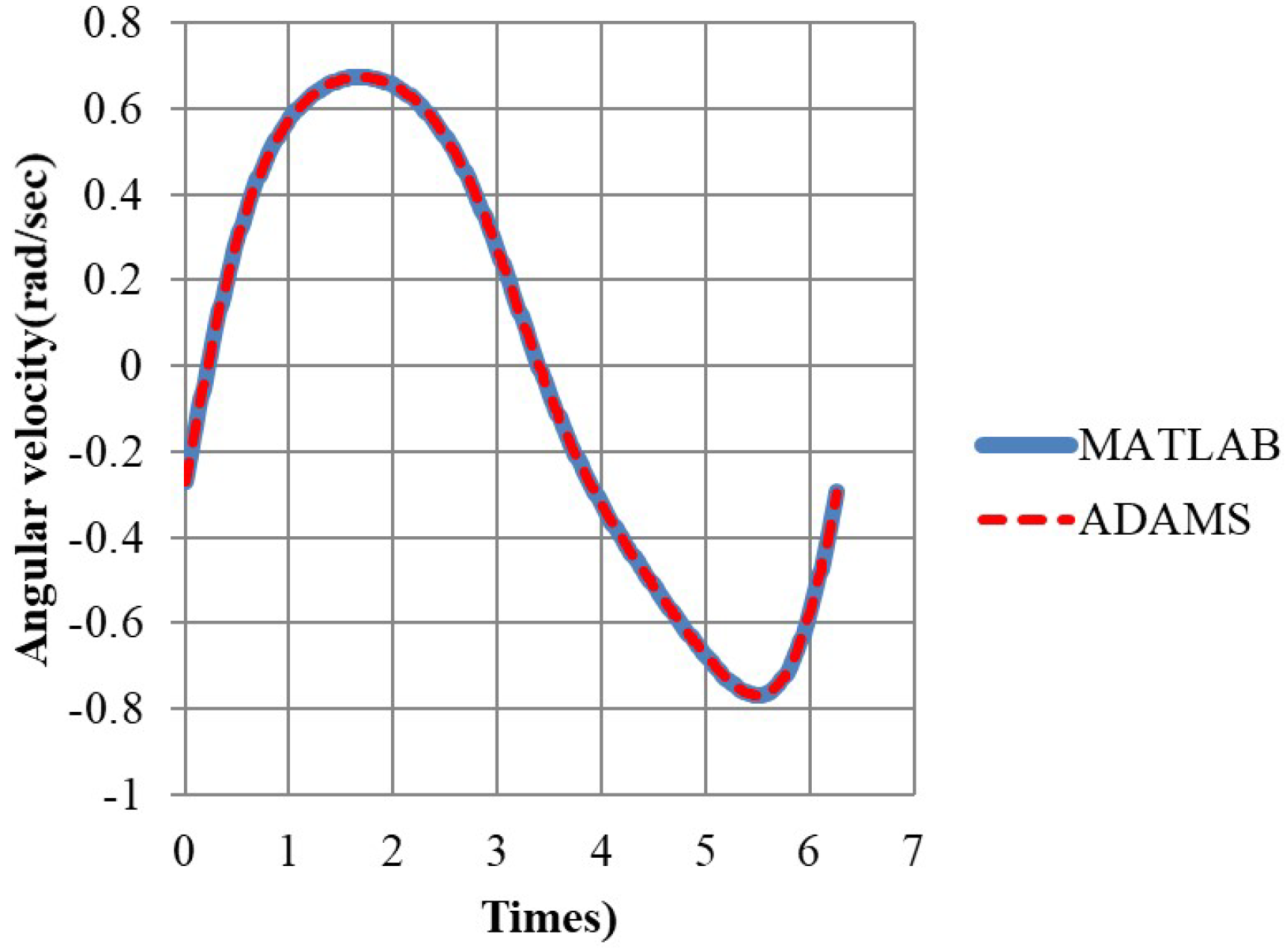
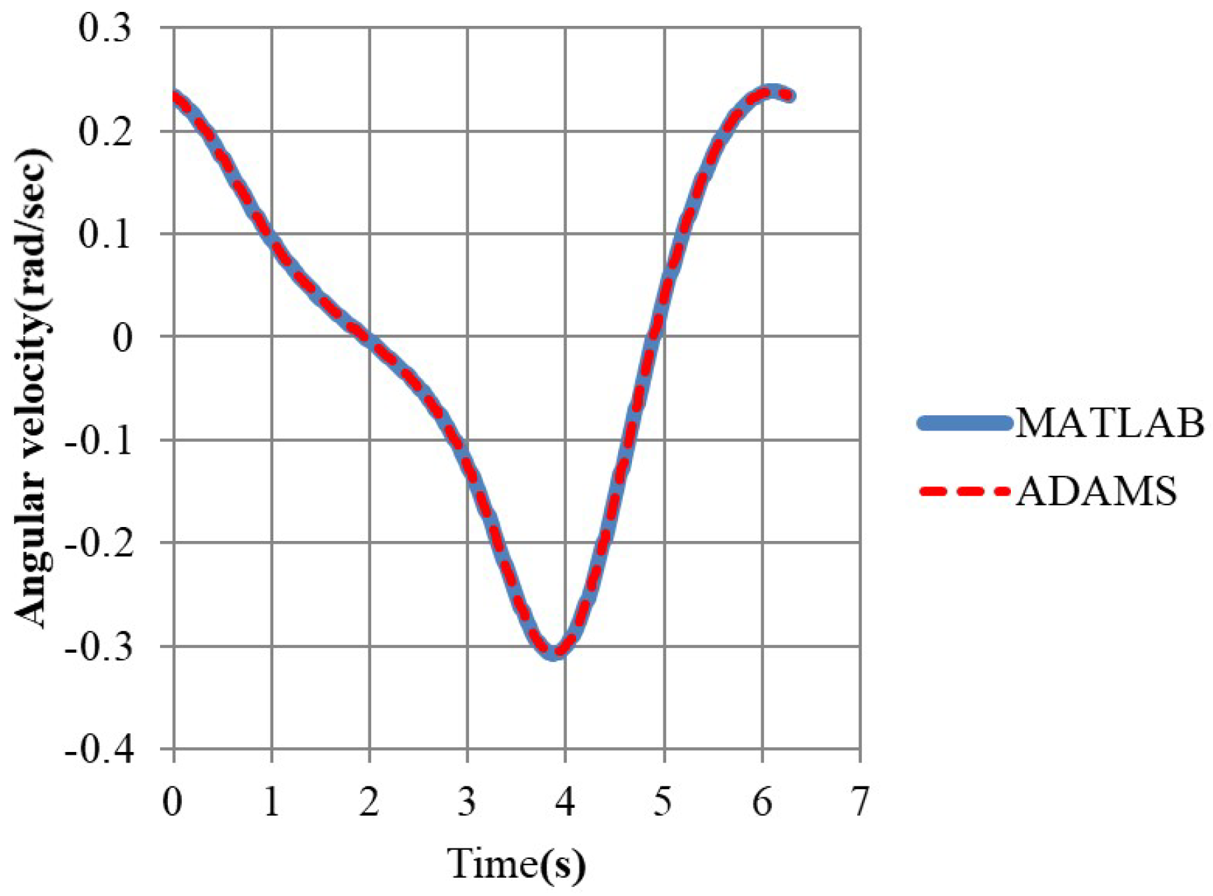
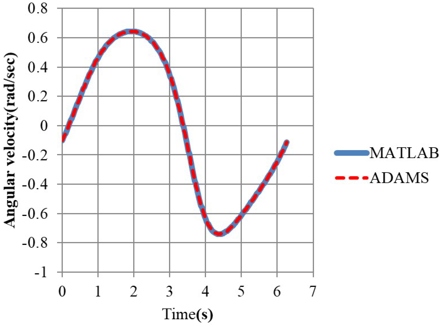
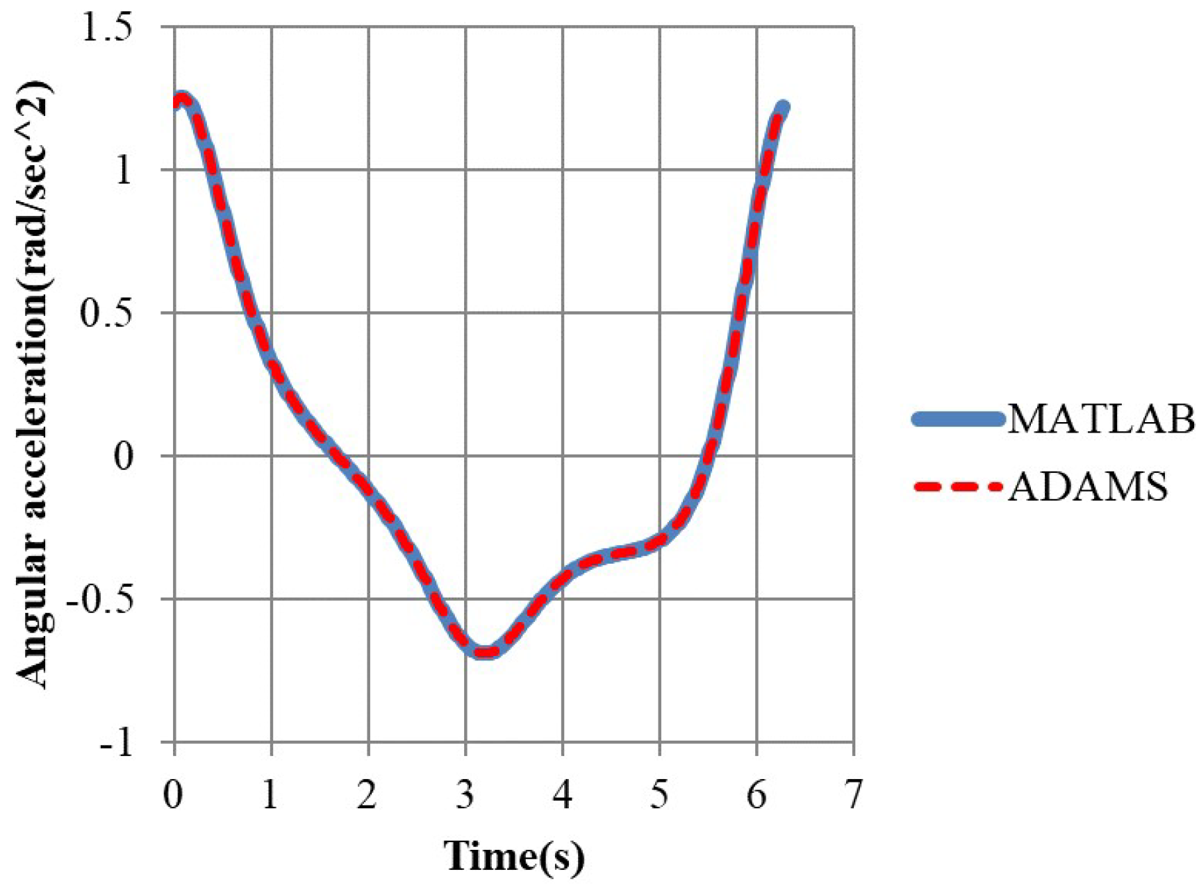
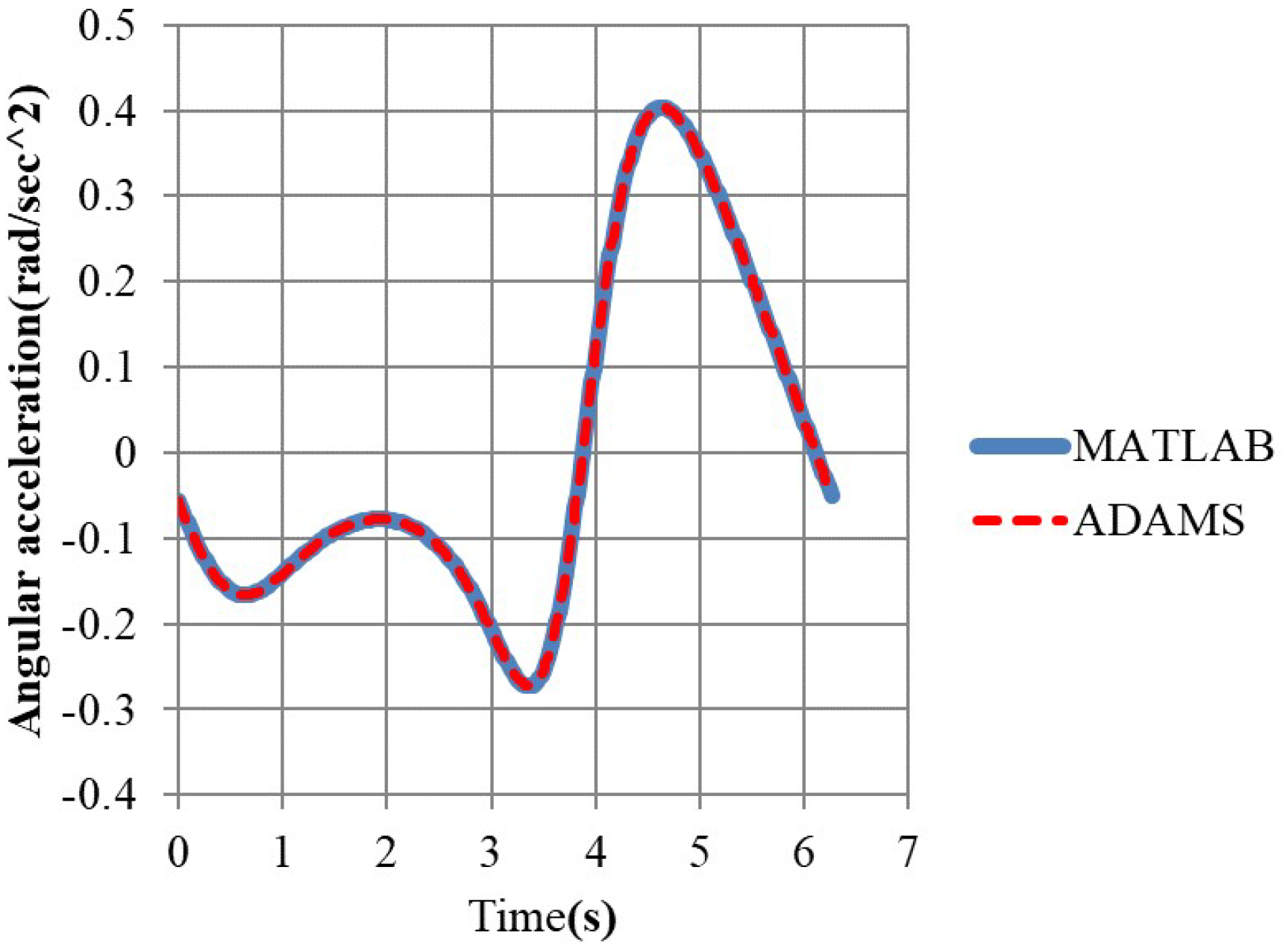
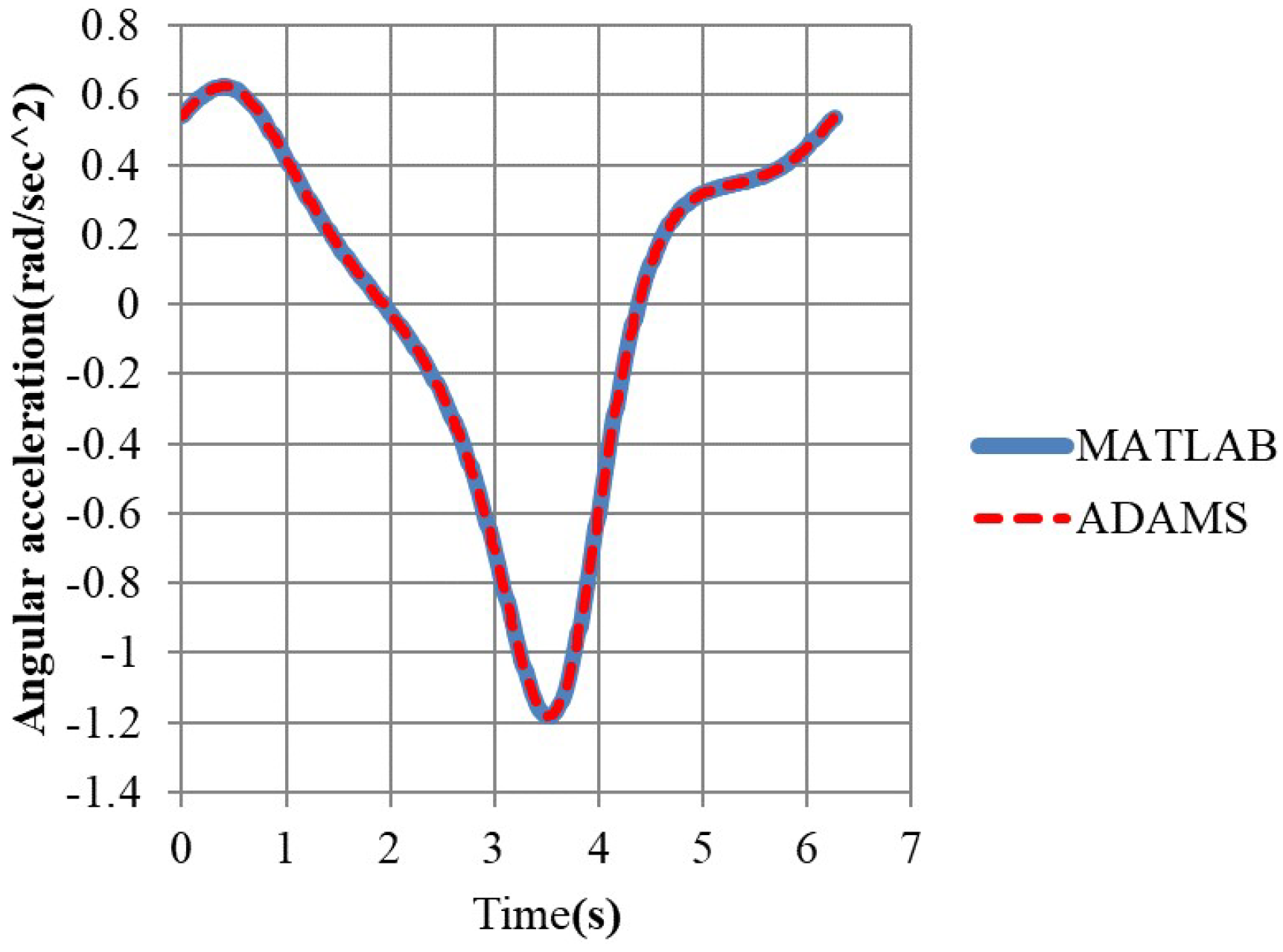
We input the same parameters into the commercial software ADAMS to justify our modeling. Comparison of the computation results from our mathematical formulas on MATLAB with that from the commercial software ADAMS is shown in Figure 6, Figure 7, Figure 8, Figure 9, Figure 10, Figure 11, Figure 12 and Figure 13.
Comparison of our calculation results based on the mathematical formulas derived in Section 2.1 with that by commercial ADAMS shows that our modeling correct and reliable.

3.2. Comparison of the Linkage Lengths before DE Optimization with That after DE Optimization

Our DE search results on the optimization problem of the objective function
f ( r 3 , r 4 , r 5 , r 6 ) = max 0 θ 2 2 π | α 4 ( r 3 , r 4 , θ 2 ) | + max 0 θ 2 2 π | α 6 ( r 5 , r 6 , θ 2 ) |
of the maximal absolute values | α 4 | and | α 6 | of angular acceleration of the output-links of a commercially available CDLS are shown in Table 2.
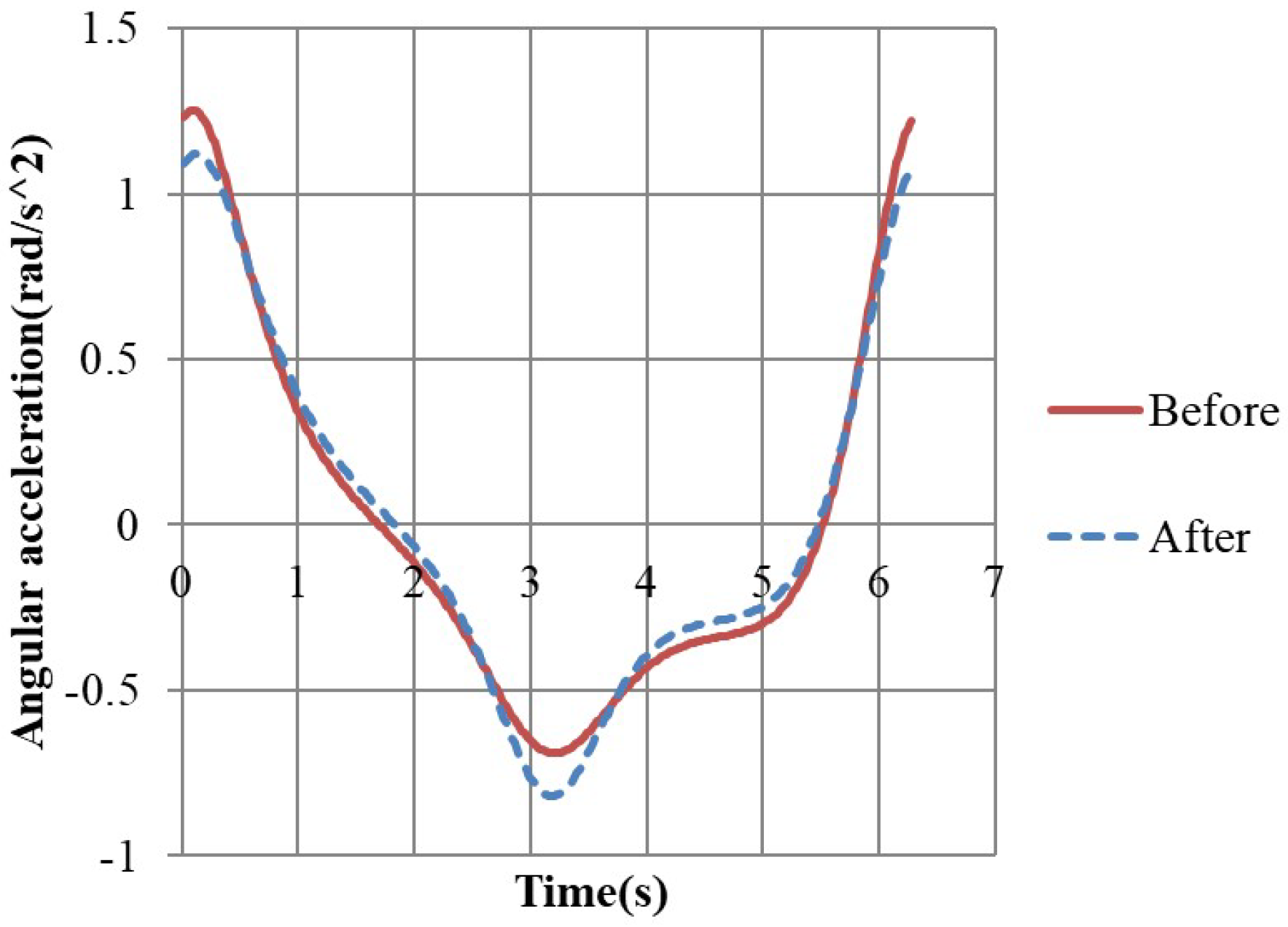
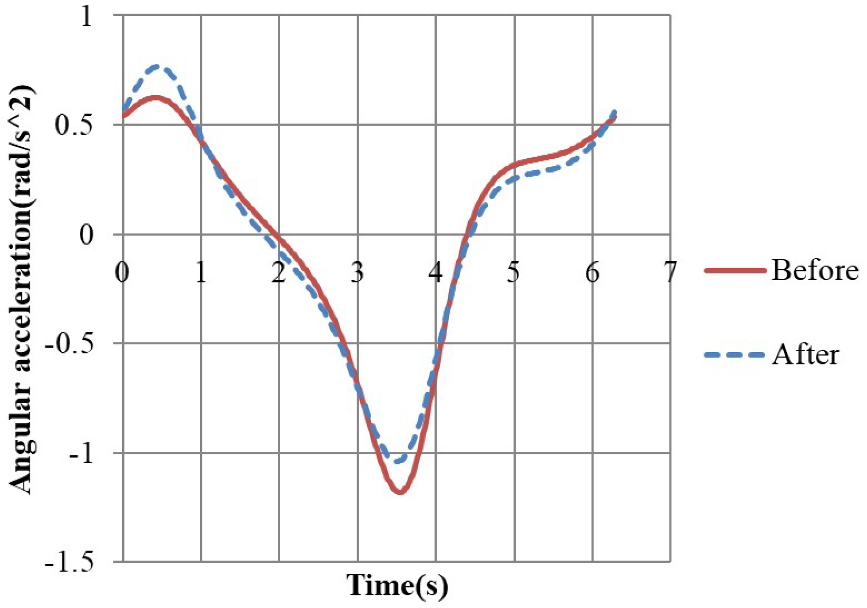
We notice that, on Figure 14 and Figure 15, the maximal absolute values  | α 4 | and | α 6 | of angular acceleration of the output-links respectively on the driver side and on the passenger side of CDLS become smaller after our DE optimization.
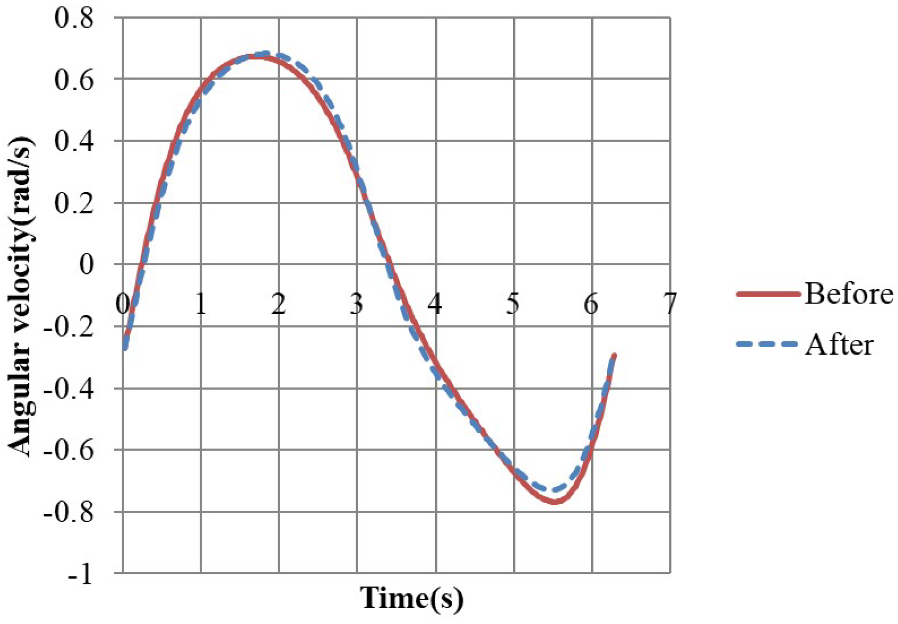
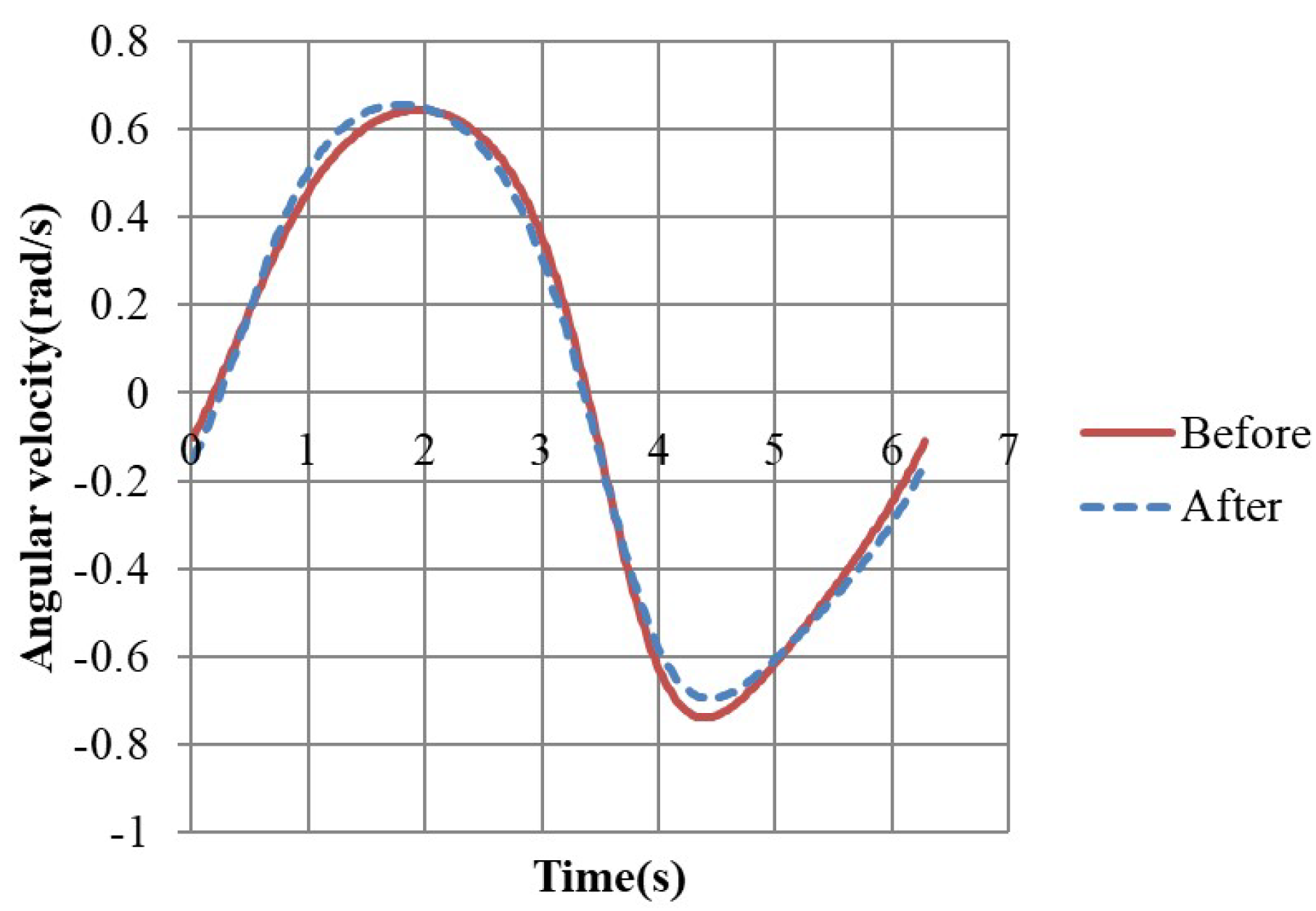
We notice that, on Figure 16 and Figure 17, both the angular velocities of the output-links respectively on the driver side and on the passenger side of CDLS do not change much after our DE optimization.
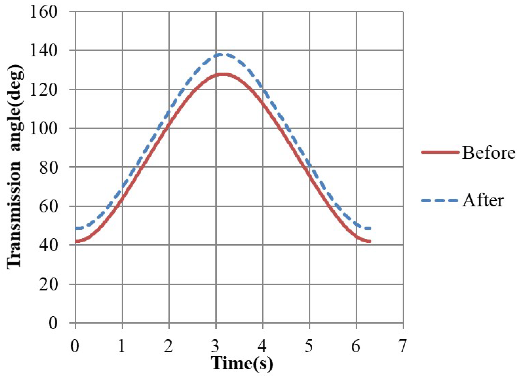
We notice that, on Figure 18 and Figure 19, both transmission angles of CDLS become closer to π / 2 (rad) or 90° after our DE optimization. In fact, this optimization slightly improves the effective torques of the output links of CDLS. See Table 3.
The resulting reduction of deviation of transmission angles from π/2 clearly shows us that the torque-efficiency by the input-link is improved. Thus improvement on the steadiness of a linkage system for vehicle wipers could also reduce the possible material fatigue of a linkage system.
Notice that, on Table 4, our optimization reduces the maximal magnitude max   | α 4 | of angular acceleration of the output-link on the driver side of CDLS by 10.69%. Besides, notice that, on Table 5, our optimization reduces the maximal magnitude max   | α 6 | of angular acceleration of the output-link on the passenger side of CDLS by 12.10%.

4. Discussion

In this article, we have explained how to improve the steadiness of a linkage system for vehicle wipers without weakening its normal function. This improvement is based on an optimization process on the maximal absolute values of angular acceleration of the output-links of a linkage system. We have demonstrated how to optimize the maximal magnitude of angular acceleration of the output-links of a commercially available center driven linkage system (CDLS) for vehicle wipers using a Differential Evolution type search method. This improvement on the steadiness of a linkage system for vehicle wipers could reduce the possible material fatigue of a linkage system. It also improves the torque-efficiency of the input-link.
This optimization problem is related to another problem which we now discuss. Reducing the unpleasant rubber wiper noise on vehicle windshield has been an interesting research topic over the past few decades [28,29,30,31,32,33,34,35,36,37,38,39,40,41,42]. Some simple spring-mass models for the vibration of rubber wiper were presented for simulations before [32,39,41]. Improvement on the electrical motor of a linkage system for rubber wipers was discussed in [42].
Since rubber wipers are made of the almost hyper-elastic material “rubber” [43,44,45], it is natural to expect that the mathematical theories of Elasticity Mechanics [46,47,48], and the mathematical theories of Partial Differential Equations [49,50,51,52], should be helpful for us to understand the complicated vibration of rubber wiper. In our earlier research [21], we seriously analyze the Elasticity Mechanics and Physics of rubber wiper on convex windshield through mathematical theories of Partial Differential Equations and through physical aspects of vibration [46,47,48,49,50,51,52,53]. We discovered two important mathematical formulas
λ + 2 μ ρ n 2 l   H z   ( Class   I )   and   μ ρ n 2 l   H z   ( Class   II )
For two classes of “characteristic vibration frequencies” of rubber wiper on convex windshield through mathematical analysis of the partial differential system of Lame equations
2 v t 2 = ( λ + μ ) ρ ( v 1 x 1 + v 2 x 2 + v 3 x 3 ) + μ ρ ( 2 v x 1 2 + 2 v x 2 2 + 2 v x 3 2 )
= ( λ + μ ) ρ ( d i v   v ) + μ ρ Δ v
here ρ   k g / m 3 and l   m are respectively the density and the length of the rubber wiper. The constants λ and μ are the “Lame coefficients” of the rubber wiper. These material constants are related to “the Young modulus E ” and “the Poisson ratio (the coefficient of transverse contraction) σ ” of rubber wiper as follows:
λ = σ E ( 1 + σ ) ( 1 2 σ )   and   μ = E 2 ( 1 + σ )
When rubber wipers move back and forth on a vehicle windshield, sharp wiper noise is generated around each reversal of the motion of rubber wipers on windshield. Usually the maximal magnitude of angular acceleration of an output-link of a CDLS happens around each reversal of the motion of this output-link. See Figure 14 and Figure 15.
Since larger angular acceleration of an output-link usually would lead to greater normal/shear stress on the rubber wiper associated with this output-link, we expect that reduction of the maximal magnitude of angular acceleration of an output-link would also be helpful for reducing the amplitudes of sound waves of wiper noise around each reversal of the motion of this output-link. Further studies on these topics should be interesting.

Author Contributions

Methodology, T.-J.C. and Y.-J.H.; Software, C.-H.L. and J.-Y.W. All authors have read and agreed to the published version of the manuscript.

Funding

This research was funded by the National Science and Technology Council of Taiwan Government, grants 110-2115-M-006-008- and 111-2115-M-006-008-.

Data Availability Statement

Not applicable.

Conflicts of Interest

The authors declare no conflict of interest.

References

  1. McCarthy, J.M.; Soh, G.S. Geometric Design of Linkages, 2nd ed.; Springer: New York, NY, USA, 2010. [Google Scholar]
  2. Storn, R.; Price, K.V. Differential Evolution—A Simple and Efficient Adaptive Scheme for Global Optimization over Continuous Spaces; Technical Report, TR-95-012; International Computer Science Institute (ICSI) of University of California: Berkeley, CA, USA, 1995. [Google Scholar]
  3. Storn, R.; Price, K.V. Differential Evolution—A Simple and Efficient Heuristic for Global Optimization over Continuous Spaces. J. Glob. Optim. 1997, 11, 341–359. [Google Scholar] [CrossRef]
  4. Storn, R.; Price, K.V. Differential Evolution: A Practical Approach to Global Optimization; Springer: Berlin/Heidelberg, Germany, 2005. [Google Scholar]
  5. Fan, Y.-F.; Lampinen, J. A Trigonometric Mutation Operation to Differential Evolution. J. Glob. Optim. 2003, 27, 105–129. [Google Scholar] [CrossRef]
  6. Tizhoosh, H.R. Opposition-Based Learning: A New Scheme for Machine Intelligence. In Proceedings of the International Conference on Computational Intelligence for Modeling Control and Automation—CIMCA, Vienna, Austria, 28–30 November 2005. [Google Scholar]
  7. Tizhoosh, H.R. Reinforcement Learning based on Actions and Opposite Actions. In Proceedings of the ICGST International Conference on Artificial Intelligence and Machine Learning (AIML-05), Cairo, Egypt, 10–21 December 2005. [Google Scholar]
  8. Tizhoosh, H.R. Opposition-based Reinforcement Learning. J. Adv. Comput. Intell. Intell. Inform. 2006, 10, 578–585. [Google Scholar] [CrossRef]
  9. Rahnamayan, S.; Tizhoosh, H.R.; Salama, M.M.A. Opposition Based Differential Evolution. IEEE Trans. Evol. Comput. 2008, 12, 64–79. [Google Scholar] [CrossRef] [Green Version]
  10. Das, S.; Abraham, A.; Chakraborty, U.K.; Konar, A. Differential Evolution using a Neighborhood Based Mutation Operator. IEEE Trans. Evol. Comput. 2009, 13, 526–553. [Google Scholar] [CrossRef] [Green Version]
  11. Qin, A.K.; Huang, V.L.; Suganthan, P.N. Differential Evolution Algorithm with Strategy Adaptation for Global Numerical Optimization. IEEE Trans. Evol. Comput. 2009, 13, 398–417. [Google Scholar] [CrossRef]
  12. Brest, J.; Sepesy Maučec, M. Self-Adaptive Differential Evolution Algorithm Using Population Size Reduction and Three Strategies. Soft Comput. 2011, 15, 2157–2174. [Google Scholar] [CrossRef]
  13. Lou, Y.; Yuen, S.Y.; Chen, G. Non-Revisiting Stochastic Search Revisited: Results, Perspectives, and Future Directions. Swarm Evol. Comput. 2021, 61, 100828. [Google Scholar] [CrossRef]
  14. Črepinšek, M.; Liu, S.-H.; Mernik, M.; Ravber, M. The Trap of Sisyphean Work in Differential Evolution and How to Avoid It. In Differential Evolution: From Theory to Practice, 1st ed.; Vinoth Kumar, B., Oliva, D., Suganthan, P.N., Eds.; Springer: Singapore, 2022; pp. 137–174. [Google Scholar]
  15. Das, S.; Suganthan, P.N. Differential Evolution: A Survey of the State-of-the-Art. IEEE Trans. Evol. Comput. 2011, 15, 4–31. [Google Scholar] [CrossRef]
  16. Das, S.; Mullick, S.S.; Suganthan, P.N. Recent Advances in Differential Evolution—An Updated Survey. Swarm Evol. Comput. 2016, 27, 1–30. [Google Scholar] [CrossRef]
  17. Karol R.Opara, K.O.; Arabas, J. Differential Evolution: A Survey of Theoretical Analyses. Swarm Evol. Comput. 2019, 44, 546–558. [Google Scholar] [CrossRef]
  18. Rudolph, G. Convergence of Evolutionary Algorithms in General Search Spaces. Proceedings of IEEE International Conference on Evolutionary Computation, Nagoya, Japan, 20–22 May 1996. [Google Scholar]
  19. Hu, Z.; Su, Q.; Yang, X.; Xiong, Z. Not Guaranteeing Convergence of Differential Evolution on a Class of Multimodal Functions. Appl. Soft Comput. 2016, 41, 479–487. [Google Scholar] [CrossRef]
  20. Hu, Z.; Xiong, S.; Su, Q.; Fang, Z. Finite Markov Chain Analysis of Classical Differential Evolution Algorithm. J. Comput. Appl. Math. 2014, 268, 121–134. [Google Scholar] [CrossRef]
  21. Chen, T.-J.; Hong, Y.-J. Geometric Analysis of the Vibration of Rubber Wiper Blade. Taiwan. J. Math. 2021, 25, 491–516. [Google Scholar] [CrossRef]
  22. Tang, Y.; Liu, Z.; He, B. Optimization Design for Crank-rocker Mechanism Based on Genetic Algorithm. In Proceedings of the 2012 Second International Conference on Intelligent System Design and Engineering Application, Sanya, China, 6–7 January 2012. [Google Scholar]
  23. Balli, S.S.; Chand, S. Transmission angle in mechanisms. Mech. Mach. Theory 2002, 37, 175–195. [Google Scholar] [CrossRef]
  24. Wang, Y.; Cai, Z.; Hang, Q. Differential Evolution with Composite Trial Vector Generation Strategies and Control Parameters. IEEE Trans. Evol. Comput. 2011, 15, 55–66. [Google Scholar] [CrossRef]
  25. Ma, C.-F. Optimization Methods and MATLAB Programming; Science Press, Chinese Academy of Sciences: Beijing, China, 2010. [Google Scholar]
  26. Arafa, M.; Sallam, E.A.; Fahmy, M.M. An enhanced differential evolution optimization algorithm. In Proceedings of the 2014 Fourth International Conference on Digital Information and Communication Technology and its Applications (DICTAP), Bangkok, Thailand, 6–8 May 2014. [Google Scholar]
  27. Electronic Code of Federal Regulations. Available online: https://www.ecfr.gov/cgi-bin/text-idx?SID=7d443eb75ceba033fed91e90f816b574&node=se49.6.571_1104&rgn=div8 (accessed on 10 October 2020).
  28. Begout, M. Les Problèmes Liés au Frottement Élastomère-Verre dans L’Automobile. Ph.D. Thesis, Université Paul Sabatier de Toulouse, Toulouse, France, 1979. [Google Scholar]
  29. Okura, S.; Sekiguchi, T.; Oya, T. Dynamic Analysis of Blade Reversal Behavior in a Windshield Wiper System; SAE 2000 World Congress 2000, Technical Paper 2000-01-0127; SAE International: Warrendale, PA, USA, 2000. [Google Scholar]
  30. Goto, S.; Takahashi, H.; Oya, T. Investigation of wiper blade squeal noise reduction measures. In SAE 2001 Noise & Vibration Conference & Exposition; Technical Paper 2001-01-1410; SAE International: Warrendale: Warrendale, PA, USA, 2001. [Google Scholar]
  31. Goto, S.; Takahashi, H.; Oya, T. Clarification of the Mechanism of Wiper Blade Rubber Squeal Noise Generation. JSAE Rev. 2001, 22, 57–62. [Google Scholar] [CrossRef]
  32. Grenouillat, R.; Leblanc, C. Simulation of chatter vibrations for wiper systems. In SAE 2002 World Congress & Exhibition; Technical Paper 2002-01-1239; SAE International: Warrendale, PA, USA, 2002. [Google Scholar]
  33. Berger, S.; Sinou, J.-J.; Aubry, E. Model of Chatter Vibrations and Stability Analysis of a Non-linear Wiper System. Int. Rev. Mech. Eng. 2008, 2, 349–356. [Google Scholar]
  34. Stein, G.J.; Zahoransky, R.; Múčka, P. On Dry Friction Modelling and Simulation in Kinematically Excited Oscillatory Systems. J. Sound Vib. 2008, 311, 74–96. [Google Scholar] [CrossRef]
  35. Bódai, G.; Goda, T.J. Friction Force Measurement at Windscreen Wiper/Glass Contact. Tribol. Lett. 2012, 45, 515–523. [Google Scholar] [CrossRef]
  36. Nechak, L.; Berger, S.; Aubry, E. Prediction of Random Self Friction-Induced Vibrations in Uncertain Dry Friction Systems Using a Multi-Element Generalized Polynomial Chaos Approach. J. Vib. Acoust. 2012, 134, 041015. [Google Scholar] [CrossRef]
  37. Min, D.; Jeong, S.; Yoo, H.H.; Kang, H.; Park, J. Experimental Investigation of Vehicle Wiperblade’s Squeal Noise Generation due to Windscreen Waviness. Tribol. Int. 2014, 80, 191–197. [Google Scholar] [CrossRef]
  38. Bódai, G.; Goda, T.J. Sliding Friction of Wiper Blade: Measurement, FE Modeling and Mixed Friction Simulation. Tribol. Int. 2014, 70, 63–74. [Google Scholar] [CrossRef]
  39. Lancioni, G.; Lenci, S.; Galvanetto, U. Dynamics of windscreen wiper blades: Squeal noise, reversal noise and chattering. Int. J. Non-Linear Mech. 2015, 80, 132–143. [Google Scholar] [CrossRef]
  40. Reddyhoff, T.; Dober, O.; Rouzic, J.L.; Gotzen, N.-A.; Parton, H.; Dini, D. Friction Induced Vibration in Windscreen Wiper Contacts. J. Vib. Acoust. 2015, 137, 041009. [Google Scholar] [CrossRef]
  41. Unno, M.; Shibata, A.; Yabuno, H.; Yanagisawa, D.; Nakano, T. Analysis of the Behavior of a Wiper Blade around the Reversal in Consideration of Dynamic and Static Friction. J. Sound Vib. 2017, 393, 76–91. [Google Scholar] [CrossRef]
  42. Viscardi, M.; Di Leo, R.; Ciminello, M.; Brandizzi, M. Preliminary Experimental/Numerical Study for the Vibration Annoyance Control of a Windshield Wiper Mechanical System through a Synchronized Switch Shunt Resonator (SSSR) Technology. J. Theor. Appl. Mech. 2018, 56, 283–296. [Google Scholar] [CrossRef] [Green Version]
  43. Muhr, A.H. Modeling the Stress-Strain Behavior of Rubber. Rubber Chem. Technol. 2005, 78, 391–425. [Google Scholar] [CrossRef]
  44. Wang, W.; Chen, S. Hyperelasticity, Viscoelasticity, and Nonlocal Elasticity Govern Dynamic Fracture in Rubber. Phys. Rev. Lett. 2005, 95, 144301. [Google Scholar] [CrossRef]
  45. Yang, C.; Persson, B.N.J. Molecular Dynamics Study of Contact Mechanics: Contact Area and Interfacial Separation from Small to Full Contact. Phys. Rev. Lett. 2008, 100, 024303. [Google Scholar] [CrossRef] [Green Version]
  46. Frankel, T. The Geometry of Physics; Cambridge University Press: Cambridge, UK, 2004. [Google Scholar]
  47. Chaichian, M.; Merches, I.; Tureanu, A. Mechanics; Springer: Berlin/Heidelberg, Germany, 2012. [Google Scholar]
  48. Ernst, E. The Boussinesq Form of Saint-Venant’s Principle. Math. Model. Methods Appl. Sci. 2000, 10, 863–875. [Google Scholar] [CrossRef]
  49. Gilbarg, D.; Trudinger, N.S. Elliptic Partial Differential Equations of Second Order; Springer: Berlin/Heidelberg, Germany, 2001. [Google Scholar]
  50. Alinhac, S. Hyperbolic Partial Differential Equations; Springer: New York, NY, USA, 2009. [Google Scholar]
  51. Evans, L.C. Partial Differential Equations; American Mathematical Society: Providence, RI, USA, 2010. [Google Scholar]
  52. Serov, V. Fourier Transform and Their Applications to Mathematical Physics; Springer International Publishing AG: New York, NY, USA, 2017. [Google Scholar]
  53. Rossing, T.D.; Fletcher, N.H. Principles of Vibration and Sound; Springer: New York, NY, USA, 2004. [Google Scholar]
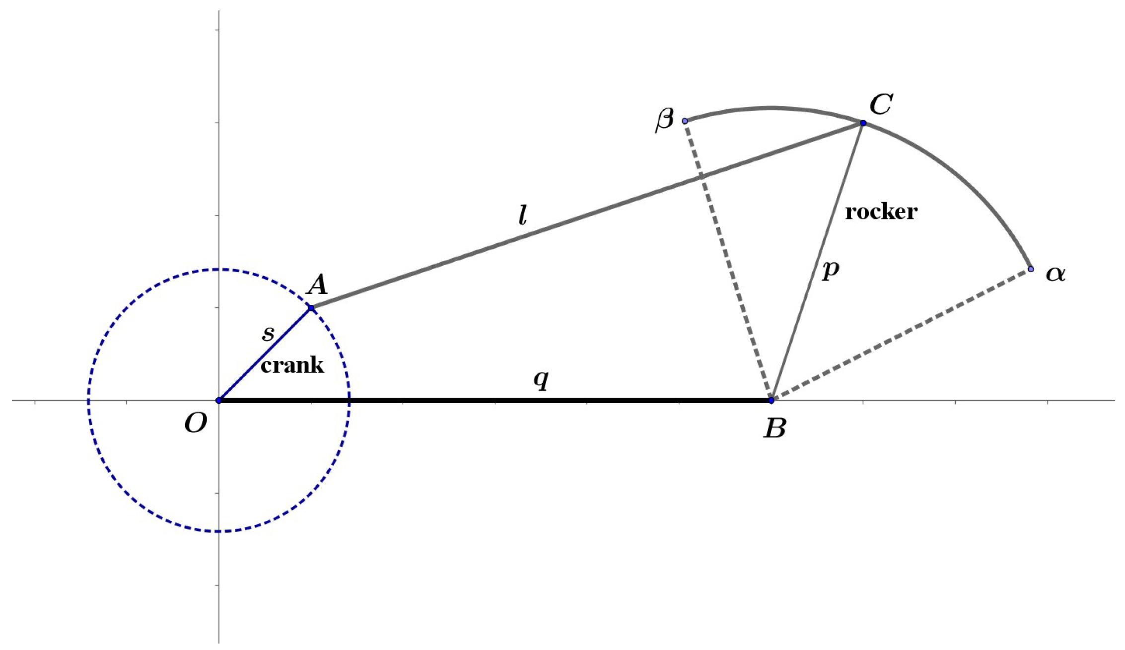
Figure 1. Crank-rocker linkage system.
Applsci 13 00332 g001
Figure 2. Usual stages of DE search algorithm.
Applsci 13 00332 g002
Figure 3. Flowchart of our research method.
Applsci 13 00332 g003
Figure 4. Structure of a center driven linkage system (CDLS).
Applsci 13 00332 g004
Figure 5. Simplified planar model of the CDLS.
Applsci 13 00332 g005
Figure 6. Comparison of our modeling computation with that of ADAMS on ω 3 .
Applsci 13 00332 g006
Figure 7. Comparison of our modeling computation with that of ADAMS on ω 4 .
Applsci 13 00332 g007
Figure 8. Comparison of our modeling computation with that of ADAMS on ω 5 .
Applsci 13 00332 g008
Figure 9. Comparison of our modeling computation with that of ADAMS on ω 6 .
Applsci 13 00332 g009
Figure 10. Comparison of our modeling computation with that of ADAMS on α 3 .
Applsci 13 00332 g010
Figure 11. Comparison of our modeling computation with that of ADAMS on α 4 .
Applsci 13 00332 g011
Figure 12. Comparison of our modeling computation with that of ADAMS on α 5 .
Applsci 13 00332 g012
Figure 13. Comparison of our modeling computation with that of ADAMS on α 6 .
Applsci 13 00332 g013
Figure 14. The angular acceleration α 4 of the driver side output-link of CDLS before/after DE optimization.
Applsci 13 00332 g014
Figure 15. The angular acceleration α 6 of the passenger side output-link of CDLS before/after DE optimization.
Applsci 13 00332 g015
Figure 16. The angular velocity ω 4 of the driver side output-link of CDLS before/after DE optimization.
Applsci 13 00332 g016
Figure 17. The angular velocity ω 6 of the driver side output-link of CDLS before/after DE optimization.
Applsci 13 00332 g017
Figure 18. The transmission angle μ 4 of the driver side output-link of CDLS before/after DE optimization.
Applsci 13 00332 g018
Figure 19. The transmission angle μ 6 of the passenger side output-link of CDLS before/after DE optimization.
Applsci 13 00332 g019
Table 1. Parameter values used in simulations.
r 1 (mm) r 11 (mm) r 3 (mm) r 4 (mm) r 5 (mm) r 6 (mm) θ 1 (mm) r 2 (mm) ω 2
(rad/s)
α 2
(rad/s2)
210.5206.820966.8206.069.9 207 π 180 4510
Table 2. Linkage lengths before/after DE optimization.
r 3 (mm) r 4 (mm) r 5 (mm) r 6 (mm)
Linkage length before DE209.066.8206.069.9
Linkage length after DE202.066.7196.469.5
Table 3. The deviation of μ 4 and μ 6 respectively from π/2 before/after DE optimization.
max 0 θ 2 2 π | μ 4 π 2 |
min 0 θ 2 2 π | μ 6 π 2 |
Before DE0.8379(rad)0.8232(rad)
After DE0.8377(rad)0.8205(rad)
Table 4. α 4 and ω 4 of the driver side output-link of CDLS before/after DE optimization.
max 0 θ 2 2 π α 4
min 0 θ 2 2 π α 4
max 0 θ 2 2 π ω 4
min 0 θ 2 2 π ω 4
Before DE1.254 (rad/s2)−0.690 (rad/s2)0.674 (rad/s2)−0.769 (rad/s2)
After DE1.120 (rad/s2)−0.819 (rad/s2)0.683 (rad/s2)−0.730 (rad/s2)
Change−10.69%18.70%1.34%−5.07%
Table 5. α 6 and ω 6 of the passenger side output-link of CDLS before/after DE optimization.
max 0 θ 2 2 π α 6
min 0 θ 2 2 π α 6
max 0 θ 2 2 π ω 6
min 0 θ 2 2 π ω 6
Before DE0.624(rad/s2)−1.182(rad/s2)0.644(rad/s)−0.739(rad/s)
After DE0.767(rad/s2)−1.039(rad/s2)0.657(rad/s)−0.696(rad/s)
Change22.92%−12.10%2.02%−5.82%
Disclaimer/Publisher’s Note: The statements, opinions and data contained in all publications are solely those of the individual author(s) and contributor(s) and not of MDPI and/or the editor(s). MDPI and/or the editor(s) disclaim responsibility for any injury to people or property resulting from any ideas, methods, instructions or products referred to in the content.