A Self-Adaptive Approximated-Gradient-Simulation Method for Black-Box Adversarial Sample Generation

Abstract

Deep neural networks (DNNs) have famously been applied in various ordinary duties. However, DNNs are sensitive to adversarial attacks which, by adding imperceptible perturbation samples to an original image, can easily alter the output. In state-of-the-art white-box attack methods, perturbation samples can successfully fool DNNs through the network gradient. In addition, they generate perturbation samples by only considering the sign information of the gradient and by dropping the magnitude. Accordingly, gradients of different magnitudes may adopt the same sign to construct perturbation samples, resulting in inefficiency. Unfortunately, it is often impractical to acquire the gradient in real-world scenarios. Consequently, we propose a self-adaptive approximated-gradient-simulation method for black-box adversarial attacks (SAGM) to generate efficient perturbation samples. Our proposed method uses knowledge-based differential evolution to simulate gradients and the self-adaptive momentum gradient to generate adversarial samples. To estimate the efficiency of the proposed SAGM, a series of experiments were carried out on two datasets, namely MNIST and CIFAR-10. Compared to state-of-the-art attack techniques, our proposed method can quickly and efficiently search for perturbation samples to misclassify the original samples. The results reveal that the SAGM is an effective and efficient technique for generating perturbation samples.

1. Introduction

Deep neural networks (DNNs) have achieved impressive success in various ordinary duties, such as image classification [1], autonomous driving [2], and object recognition [3]. With the expansion of application domains, DNN robustness, which refers to the sensitivity of its output results to tiny changes in the input image, has become an important research field [4]. Clean images with tiny and imperception perturbation, known as adversarial examples, may cause DNNs to misclassify the label of an image [5]. Researchers have declared that this makes DNNs very vulnerable to adversarial examples. In real-world scenarios, there is a security risk for the adversarial examples in the contexts of self-driving vehicles [6], text classification [7], and medical diagnostic tests [8]. Adversarial examples are dangerous for DNNs but are also a strategy to enhance DNN robustness.

The method of generating adversarial examples that cause DNNs to give an incorrect output with high confidence is defined as an adversarial attack [9]. Adversarial attacks generally consist of two types of attacks, namely white-box [10] and black-box attacks [11]. The adversarial examples generated by white-box attacks can fool DNNs with high success rates, mainly because they have access to the internal knowledge of the DNN and the gradient obtained by backpropagation. However, in a real-world scenario, it is very impractical to have complete access to the internal information of a DNN. It is a new challenge for attackers to generate adversarial examples from the input image and output in a black-box attack, without considering the internal details of DNNs [12].

In a state-of-the-art white-box attack, the adversarial image mainly adds or subtracts adversarial examples to each point of the clean image in a sensitivity direction. Researchers have proposed that adversarial examples are generated by looking for the sensitivity gradient direction [13]. As a result, most attack methods only keep the gradient direction without considering the gradient magnitude. The sensitivity direction can be directly estimated from the loss of DNNs. However, black-box attackers cannot directly obtain the gradient and may simulate it through other schemes, such as zero-order optimization [14], evolution strategies [15], and the random search method [16]. A black-box attack can be implemented by solving an optimization problem on minimum perturbation. Normally, it is time-consuming to solve a high-dimensional optimization problem, and the mapping from probability to categories is extremely non-linear.

Based on the above considerations, we propose a self-adaptive approximated-gradient-simulation method for black-box adversarial attacks (SAGM) to generate perturbation samples. The SAGM utilizes self-adaptive differential evolution (DE) to simulate the gradient of each pixel and leverage the momentum gradient to improve its efficiency. In the process of gradient simulation, the DE parameters are self-adaptively adjusted according to the DNN confidence score. Finally, the perturbation image is continuously adjusted by approximating the gradient to achieve the attack purpose.

We compare the SAGM with other state-of-the-art attack methods in two datasets, namely MNIST [17] and Cifar10 [18]. Extensive experiments show that our proposed SAGM can achieve high attack efficiency that is comparable with other attack methods. Our attack method can generate an adversarial example faster and more efficiently than other methods. Finally, the SAGM is applied to strengthen DNN robustness.

The paper can be summarized by providing the following main contributions:

• We construct an evaluation model based on similarity and confidence score to validate the effectiveness of adversarial samples.
• We propose a method to simulate the approximated gradient using differential evolution.
• We propose a novel parameters adaptive scheme in which F and CR are adaptively adjusted to explore the sensitive gradient directions by the feedback of the evaluation model.
• We propose an adversarial-sample-generation method based on quantized gradients, preserving the magnitude and direction of the gradient, to generate an efficient sample.

The remainder of this paper is organized as follows. Section 2 reviews related work on recent white-box attacks, black-box attacks, and DE. The proposed SAGM is presented in detail in Section 3. Section 4 gives the experimental results and analysis. The last section, Section 5, is devoted to conclusions and future work.

2. Related Work

Image classification [19] is an image-processing method used to distinguish different categories of objects according to their different features. For k-category images, the model $C$ converts input image $x$ to output probability $t_n$ through a series of transfer processes in the DNN:$C\left(x\right)=t_n, n\in \left[1,k\right]$, and then selects the maximum probability to determine the image category. Therefore, image $x$ is correctly classified as t by model $C$, i.e., $C\left(x\right)=t$. Studies on adversarial examples focus on the robustness of DNN to tiny permutations in input, namely $C\left(x+\delta \right)=t, \delta \le p$. DNN robustness is detected by the $L_0$,$L_1$, and $L_{\infty }$ norm of the perturbations $\delta$. The adversarial attack is to misclassify the tiny permutations of the original image to an arbitrary category, i.e., $C\left(x+\delta \right)=t^{\prime }$. Two adversarial attack models exist depending on whether the attacker has access to the DNN structure, i.e., white-box and black-box attacks.

Some existing studies on adversarial attacks are surveyed in the following subsections.

2.1. White-Box Adversarial Attacks

In a white-box attack, the attacker has full access to the internal structure of a DNN and attacks the DNN with the adversarial samples generated by the DNN gradient. Szegedy et al. [5] first discovered an intriguing property of DNNs, noting that the input–output mappings are absolutely disconnected so that state-of-the-art DNNs are vulnerable to adversarial examples. It is possible to cause a DNN to misclassify the input images that are added to an imperceptible perturbation. These adversarial examples are explored by optimizing the box-constrained problem of the input images. The box-constrained problem is transferred into an unrestraint problem by the penalty function method, i.e., $c\left|r\right|+los{s}_f\left(x+r,l\right), s.t. x+r\in {\left[0,1\right]}^m$. The main task of the attack algorithm is to search the approximate minimum $r$ by the line search method to cause the DNN to misclassify. The reason for the existence of adversarial samples is the non-linearity and over-fitting of the DNN model. However, it is also possible that linear behavior in higher dimensions can also produce adversarial examples to misclassify the images.

Therefore, Goodfellow et al. [13] proposed a fast-gradient-sign method (FGSM) attack which generates adversarial examples to misclassify the images by the gradient of the loss function. The gradient is the derivative of the cross-entropy loss function with respect to the input image, which is obtained by the backpropagation of DNN. The input images are perturbed with the direction of the gradient, and only a one-step gradient update algorithm is performed. Therefore, an FGSM attack is very fast at generating adversarial examples. However, it is not efficient that adversarial examples fool the DNN because of the use of one-step modification in isolation. If the step is small, the perturbation preserves the properties of the input images without fooling the DNN; otherwise, the input images are converted to something else. To make the perturbation smaller and more efficient, researchers proposed multiple-iteration optimization to improve the performance of the FGSM, i.e., BIM attack [20] and PGD attack [21]. These iteration-based FGSMs tend to fall into the trap of local optima because they greedily move in the direction of the current gradient. To abscond from local optimal solutions, the momentum method is integrated into the iteration FGSM, i.e., MI-FGSM [22]. The momentum method mainly accumulates the velocity vector to maintain the previous gradient direction. Extensive experiments show that the MI-FGSM is effective in generating adversarial examples.

In the above attack methods, the adversarial examples are obtained by solving non-linear combinatorial optimization problems. However, it is difficult to solve the non-linear constraint directly via existing algorithms. Therefore, Carlini and Wagner [23] proposed a variety of representations of this non-linear constraint to accommodate optimization. CW attacks use the Adam optimizer to find adversarial examples. The results show that the Adam algorithm has faster convergence than other algorithms.

In the above attack methods, the adversarial examples are obtained by solving non-linear combinatorial optimization problems.

2.2. Black-Box Adversarial Attacks

In a black-box attack, the attacker can only access the outputs of the DNN, and access to the internal structure of the DNN is prevented. Therefore, the attacker cannot generate adversarial examples through the gradients that are obtained by backpropagation. Based on the transferability between models, the adversary constructs a surrogate model to generate adversarial examples. The trained surrogate model is attacked in a white-box attack to generate adversarial examples. Subsequently, the adversarial examples attack the actual model through the black-box attack. The effectiveness of black-box attacks depends largely on the transferability of attacks from the surrogate model to the actual model. However, it seems impractical to the attacker that a great deal of knowledge is obtained from the surrogate model. Chen et al. [24] proposed a zero-order optimization method to generate adversarial examples in black-box methods. The ZOO attack used zero-order optimization for the query gradient rather than using the first- or second-order method. Experimental results show that the ZOO attack is as effective as the CW attack and significantly surpasses existing black-box attacks via surrogate models. However, it is a very time-consuming query process evaluate the approximate gradient by adding small perturbations to 128 pixels at each iteration.

To reduce the time required, researchers performed evolution strategies to estimate the approximate gradient. Su et al. [25] proposed a one-pixel attack algorithm that applies the DE to search the suitable pixel and only modify it to perturb test images. This one-pixel modification perturbs the pixel point along an axis parallel to the n dimensions. The results show that the proposed attack method can deceive the DNN through a few modified pixels. However, the proposed attack may be perceptible to people, and it is inefficient because there are fewer pixels to modify. Lin et al. [26] proposed black-box adversarial sample generation based on DE (BMI-FGSM) to verify DNN robustness. BMIFGSM utilizes DE to explore the approximated gradient sign, converting a white-box MI-FGSM attack into a black-box MI-FSGM with an approximated gradient sign to form adversarial examples. Li et al. [27] proposed an approximated-gradient-sign method using DE for a black-box adversarial attack that searches the gradient sign by the DE algorithm. The proposed algorithm applies the neighborhood selection operations to construct the target image neighborhood and perform DE to optimize the weights between the target image and each image in the neighborhood. The above DE-based black-box attacks only retain the approximated gradient sign without keeping the gradient magnitude. Two different components may obtain the same value by the gradient sign method. Therefore, it is necessary to introduce the magnitude of the gradient to produce diverse values. The quantized gradients which retain the sign and the magnitude of the gradient have been successfully applied to distributed optimization.

2.3. Differential Evaluation

Differential evolution (DE) [28], proposed by Storn and Price, is an example of stochastic population-based computing intelligence. Recently, DE has been widely used in diverse fields, such as electrical and power systems [29], pattern recognition [30], artificial neural networks [31], robotics and expert systems [32], manufacturing science [33], image processing [34], and gene regulatory networks [35], because of its comprehensibility, robustness, convergence, and ease of use [36].

In recent years, researchers have contributed to DE performance improvement [37]. These improvements have mainly focused on mutation strategies, crossover strategies [38], and control parameters (i.e., population size NP, scaling factor F, and crossover rate CR). Extensive studies show that the parameter setting helps to improve DE performance [39]. However, the parameter setting is one of the most persistent challenges in an evolutionary algorithm (EA). An EA with better parameter values may have a greater order of magnitude than one with poor parameter values. In the field of EA, parameter-selection schemes usually include two approaches as follows: one approach is parameter turning, whereby parameter values are carefully picked out before an EA is run and cannot be changed in the process of running; and the other approach is parameter control, whereby parameter values are randomly initialized for the starting run of an EA and can be adjusted in the process of running. In the parameter-turning method, parameter values are set using the experimental method or the trial-and-error method [40]. Store and Price indicated that a good initial set of $F$ is 0.5, and the effective range of $F$ usually belongs to (0.4, 1). Georgioudakis et al. [41] revealed that the global exploitation capability and the speed of convergence are oversensitive to the parameters. Ronkkonen et al. [42] stated that Cr should be between (0, 0.2) when the function is separable, but between (0.9, 1) when the function is non-separable. According to the literature, proper parameters should be set differently for different functions. Therefore, researchers have started to take into account some self-adaptation techniques to automatically search optimal parameters for DE. The SaDE algorithm employed a self-adaptation scheme by learning from historical experiential solutions to control parameters $F$ and $Cr$. Ali et al. [43] proposed an adaption algorithm based on fitness for $F$. The calculation of $F$ is based on the requirements of a diversified search in the early stage and enhanced search in the later stage, and the formula is as follows (Equation (1)).

$$F=\{\begin{array}{c}\max \left(1,1-\left|\frac{f_{\max }}{f_{\min }}\right|\right)\hspace{1em}\hspace{1em}if\left|\frac{f_{\max }}{f_{\min }}\right|<1\\ \max \left(1,1-\left|\frac{f_{\min }}{f_{\max }}\right|\right)\hspace{1em} otherwise\end{array}$$

(1)

where the lower bound for $F$ is $l_{min}$ and $f_{min}$ and $f_{max}$ are the minimum and maximum function values of the populations in a generation, respectively. The extensive experimental results show that the self-adaptive DE outperforms the standard DE because of the less sensitive parameters in self-adaptive DE.

3. Our Proposed Algorithm

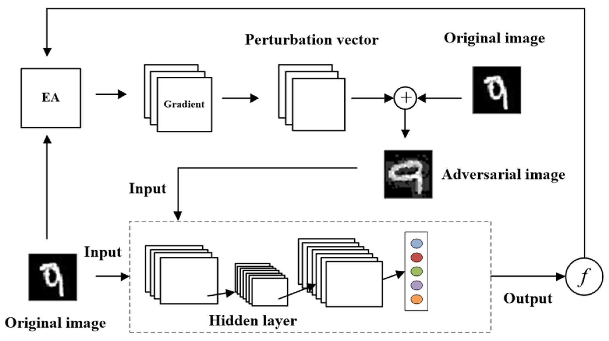
In this section, our approach, entitled self-adaptive approximated-gradient-simulation method (SAGM), is proposed to improve adversarial attacks. Its main feature is to enhance the generation of adversarial samples. Our proposed framework is depicted in Figure 1. The SAGM mainly includes two processes of simulating the approximate gradient and self-adaptive generation of adversarial samples, in which the gradient of the pixel is approximated by the evolutionary algorithms (EAs) to self-adaptively perturb the original image. These two processes are performed iteratively until the perturbed image is successfully attacked or the maximum number of runs is reached. In the following subsections, we emphasize these two processes in detail.

Figure 1. The SAGM framework.

3.1. Model Construction

In a DNN, the image $x$ is entered into the hidden layer to retrieve its features, and finally outputs the confidence vector of n categories $p\left(x,n\right)\in \left[0,1\right]$. The SAGM is a black-box attack method without concern for the DNN internal configurations; therefore, the adversarial image $x^{\prime }$ that is similar to the image $x$ belonging to category $t$ is identified as another category $t^{\prime }\left(t^{\prime }\ne t\right)$. To achieve this goal, the SAGM needs to solve the following constrained optimization problem presented in Equation (2).

$$\begin{array}{ll}minimize& D\left(x^{\prime }\right)={\Vert x^{\prime }-x\Vert }_2\\ s.t.& C\left(x^{\prime }\right)=t^{\prime }\\ & x^{\prime }=x+\delta \\ & \delta \in {[0,1]}^n\end{array}$$

(2)

The constrained optimization problem is to explore similar images with validity to implement misclassification. $C\left(x^{\prime }\right)=t^{\prime }$ is an extremely non-linear function whose purpose is to misclassify the image into category $t^{\prime }$. In other words, the confidence that the image belongs to category $t^{\prime }$(i.e.,$p\left(x^{\prime },t^{\prime }\right)$) is the highest among all categories. Based on this consideration, the non-linear function is converted to the following Equation (3) function.

$$l\left(x^{\prime }\right)=p\left(x^{\prime },t\right)-\underset{k\ne t}{\max }p\left(x^{\prime },k\right)$$

(3)

where $t$ is the category of the original image $x$,$p\left(x^{\prime },t\right)$ is confidence in the category $t$, $\underset{k\ne t}{\max }p\left(x^{\prime },k\right)$ is the maximum confidence among all categories $k$ that do not belong to category $t$.

When $l\left(x^{\prime }\right)$ is less than or equal to 0, the image is misclassified into other categories. Therefore, the converted function has the same purpose as the original function, which is to misclassify perturbed images. The constrained optimization problem (2) is transformed into the following new constrained optimization problem for optimization (Equation (4)).

$$\begin{array}{ll}minimize& D\left(x^{\prime }\right)={\Vert x^{\prime }-x\Vert }_2\\ s.t.& p\left(x^{\prime },t\right)-\underset{k\ne t}{\max p}\left(x^{\prime },k\right)\le 0\\ & x^{\prime }=x+\delta \\ & \delta \in {[0,1]}^n\end{array}$$

(4)

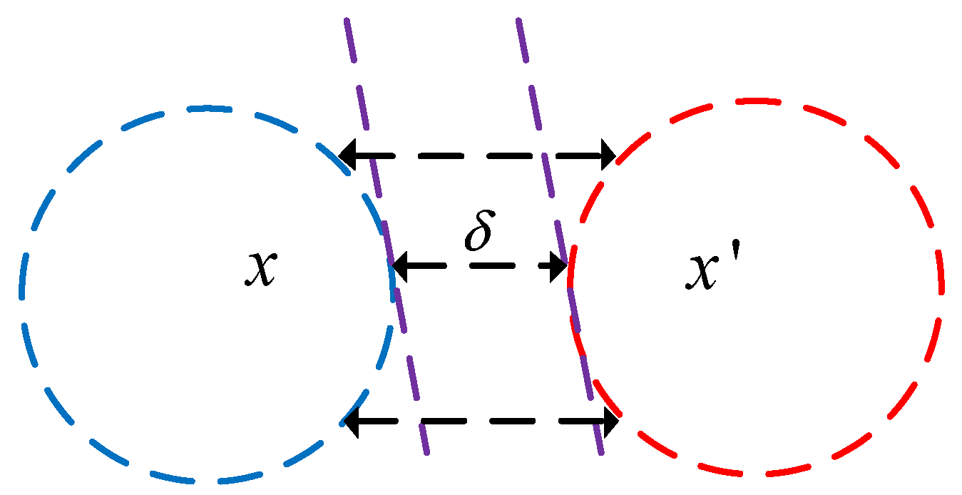
The main purpose of Equation (4) is to explore the perturbed vector $\delta$ and add it to the original image $x$ to fool the DNN. The relationship between the three parameters in Equation (4) is depicted in Figure 2.

Figure 2. The relationship between the adversarial image and the original image.

Figure 2 shows that there is an area gap between the two different categories. The red and blue dashed circles represent the feasible region $X=\left\{x|x\in \underset{k\ne t}{\max } p\left(x^{\prime }+\delta ,k\right)\right\}$ and initial solution $X_0=\left\{x|x\in p\left(x,t\right)\right\}$ of the model (4), respectively. The black dashed line indicates the gap $\delta$ between the two categories.

Based on the characteristics of the model, model (4) is converted to an unconstrained non-linear optimization problem using the exterior point method, which constructs a penalty function to penalize points in the infeasible region, as seen in the following formula (Equation (5)).

$$P(x)=\{\begin{array}{l}0,\hspace{1em}\hspace{1em}x\in X\\ M,\hspace{1em} x\notin X\end{array}$$

(5)

where $M$ is a large positive number.

The penalty function (5) can be transformed into the unconstrained problem, but there is a jump at the boundary. Therefore, to avoid this problem, the penalty function of

(4) is constructed as shown in Equation (6).

$$\begin{array}{c}{P}_{cg}(\delta )=c_g\{\left[\max \left(p(x+\delta ,t)-\underset{k\ne t}{\max } p(x+\delta ,k),0\right)\right]\\ +[\max (-\delta ,0)]+[\max (\delta -1,0)]\}\end{array}$$

(6)

In (6), $c_g$ is the penalty parameter with an ascending sequence, making $x$ gradually approach the optimal solution from the outside of the feasible region. Therefore, (4) is converted to the following augmented objective function (Equation (7)).

$$minimize f\left(\delta \right)=\parallel \delta {\parallel }_2+P_{c_g}\left(\delta \right)$$

(7)

In Equation (7), the first term on the right represents the similarity between the perturbed image $x^{\prime }$ and the image $x$, and the two images can be ensured to be identical by minimizing. The two terms on the right tend to the feasible point by imposing penalties on the infeasible points. Therefore, the solution to the adversarial image $x^{\prime }$ is actually to solve the perturbed vectors $\delta$.

3.2. Self-Adaptive Two-Step Perturbation

Perturbation based on sign gradients is an effective method for adversarial attacks. However, the sign gradient method rejects the proportion among the raw gradients, resulting in components sharing the same coefficients. Therefore, after $G$ iterations, perturbation based on a fixed step size $\alpha$ may appear in two cases, as shown in Figure 3.

Figure 3. Self-adaptive two-step perturbation.

In Figure 3, the blue and red dotted circles represent the probability contours of $x$ and $x^{\prime }$, the two black lines represent the perturbation distances $\alpha$ and $\beta$ in the gradient direction, and $x_g$ is a perturbed image after $g$ generation. Figure 3a shows that the perturbation image is not being converted into an adversarial image due to the small step size. Figure 3b shows that the perturbation image is converted into an adversarial image that is easily recognizable because of the big step size.

The main reason for this condition Is that each pixel of the original image is adjusted at a fixed learning rate to achieve the purpose of the attack. Hence, each pixel with different gradients is updated at the same learning rate. In this case, it cannot be motivated to improve the efficiency of the attack. To deal with this problem, we propose an improved two-step adaptive perturbation method to improve its efficiency. The first step is to adaptively adjust $\alpha$ to generate the temporary perturbation image $x_{g+1}^{\prime }$, and the second step is to fine-tune $x_{g+1}^{\prime }$ by adding a step size $\beta$ to move toward the boundary of the adversarial image.

In the first step, we leverage the optimal gradient in the past to guide the next-generation adaptive change of the pixel (Equation (8)).

$${\delta }_i^{\prime }={\delta }_{i-1}^{\prime }+\frac{{\delta }_{i,best}}{{\Vert {\delta }_{i,best}\Vert }_2}$$

(8)

where ${\delta }_{i,best}$ is the optimal gradient for generation $t$.

Assuming that the initial optimal gradient ${\delta }_0^{\prime }=0$, then the cumulative gradient of generation $i$ can be written as the following (Equation (9)).

$${\delta }_i^{\prime }=\sum _{i=0}^{g-1}\frac{{\delta }_{i,best}}{{\Vert {\delta }_{i,best}\Vert }_2}$$

(9)

Afterward, the ${\delta }_{g-1}^{\prime }$ and ${\delta }_g$ are linearly combined to adjust the perturbation direction and step size of the current generation (Equation (10)).

$${\delta }_g={\theta }_1\cdot {\delta }_{g-1}^{\prime }+{\theta }_2\cdot {\delta }_g$$

(10)

where ${\theta }_1$ and ${\theta }_2$ are hyperparameters that control the exponential decay rate, and ${\theta }_1+{\theta }_2=1$.

To conserve the direction and magnitude of the gradient, the perturbed vectors $\delta$ are calculated by the following Equation (11).

$$\begin{array}{l}\delta =\lambda \cdot \frac{{\delta }_g}{\max \left({\delta }_g\right)}\\ {\delta }_g=\{\begin{array}{l}sign(\delta ),\hspace{1em} if\left|\delta \right|<1\\ round (\delta ), otherwise\end{array}\end{array}$$

(11)

where $\lambda$ is a fixed parameter, $\max (\cdot )$ is the gradient maximum. Function $round (x)$ rounds the variable $x$. The main purpose of Equation (11) is to set a different step size $\alpha$ for each perturbation.

To further improve the success rate of adversarial images, the second step is adopted to fine-tune the perturbation images to approach the boundary of the target images $x_{g+2}^{\prime }$. Therefore, $\beta$ is updated by step-size derivation, as shown in Equation (12).

$${\beta }_g=\frac{⟨\mathsf{\Delta }x,\mathsf{\Delta }p⟩}{⟨\mathsf{\Delta }p,\mathsf{\Delta }p⟩}$$

(12)

where $\Delta x=x_{g+2}^{\prime }-x_{g+1}^{\prime }$,$\Delta p=p_{g+2}-p_{g+1}$, and $⟨a,b⟩$ denotes the scalar product of the vectors $a$ and $b$. $x_{g+2}^{\prime }$ is the target image that belongs to the category with the highest confidence other than the category $t$ of the original image.

3.3. Self-Adaptive Approximated Gradient Search

It is well known that black-box attacks only require access to the output, not to the network structure. The gradient cannot be obtained directly because the value of the loss function cannot be obtained. The perturbed image $x^{\prime }$ is generated by the following iterative algorithm (Equation (13)) on the basis of the original image $x$.

$$x_{g+1}^{\prime }=x_g^{\prime }+{\delta }_g$$

(13)

Assuming $p_g$ is the unit vector of ${\delta }_g$, there exists a variable ${\alpha }_g>0$ for which the equation ${\delta }_g={\alpha }_g·p_g$ holds. In the iterative algorithm, $p_g$ represents the perturbation direction of ${\delta }_g$, and ${\alpha }_g$ represents the step of the $g\mathrm{th}$ generation along the search direction $p_g$. Therefore, the iterative function is written as follows (Equation (14)).

$$x_{g+1}^{\prime }=x_g^{\prime }+{\alpha }_g\cdot sign\left({\delta }_g\right)$$

(14)

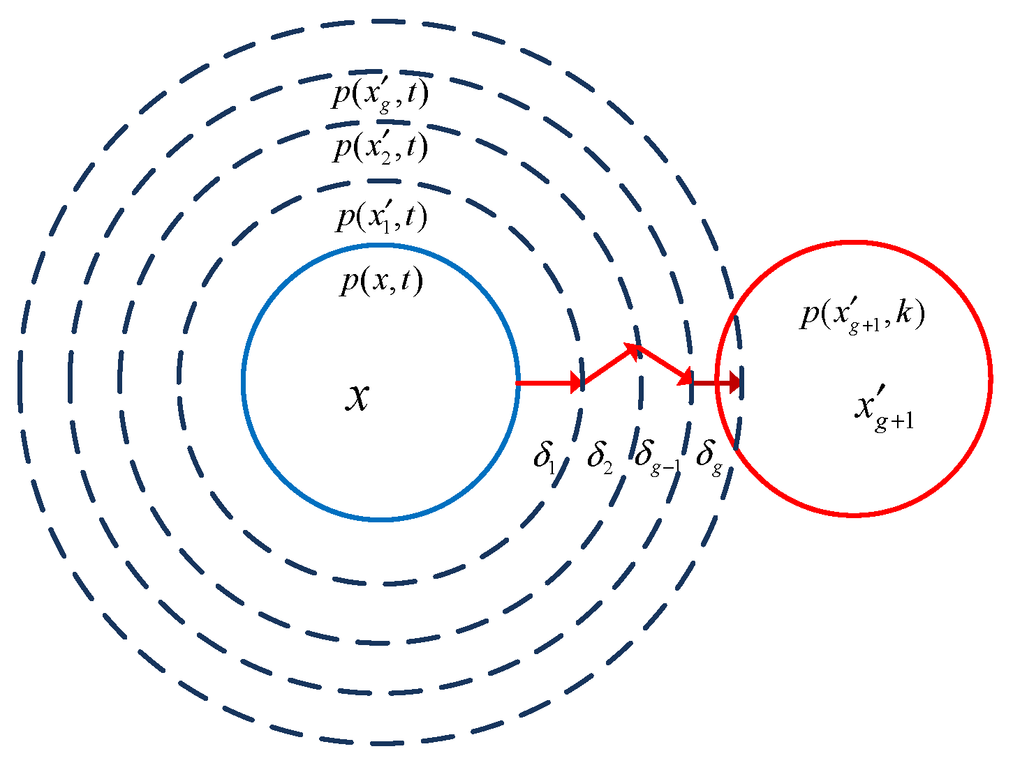
Here, the initialization value of $x_0^{\prime }$ is the clean image. The exploration process of $x^{\prime }$ is shown in Figure 4.

Figure 4. The exploration process of perturbed image.

In Figure 4, the solid blue and red circles represent the probability contour of $x$ and $x^{\prime }$, respectively. The dotted concentric circles on the left indicate that the probability of belonging to class $t$ decreases with increasing radius. The clean image is perturbed by the vector $\delta$, resulting in low probability. Meanwhile, the probability of other categories will gradually increase. When the probability of belonging to class $t$ drops to a certain threshold, an adversarial image may be generated.

Based on the above analysis, a self-adaptive DE is proposed to simulate the perturbed vectors ${\delta }_g$. Differential evolution (DE) [28], proposed by Storn and Price, has been widely used to solve numerical optimization problems because of its simplicity, robustness, convergence, and ease of use. The three steps in DE, namely mutation, crossover, and selection, are computed repeatedly until the termination criterion is satisfied. Mutation produces a mutant vector through mutation strategies, the crossover is the process of recombination between the mutant vector and the target vector, and selection is to preserve the optimal individuals for the next generation according to the greedy choice method.

In the SAGM, we utilize adaptive DE to explore the perturbed vectors. The initial perturbed vector between −1 and 1 is generated using uniformly distributed randomization, and its dimension is consistent with the dimension of the input image. Each element of the initial vector ${\delta }_0$ is generated by Equation (15).

$${\delta }_0=\min +rand(0,1)\cdot (\max -\min )$$

(15)

where $min$ and $max$ are the minimum and maximum of the gradient, respectively, and $rand(0, 1)$ is a random number between 0 and 1.

After initialization, a mutant vector is produced with respect to the target vector. In each generation of mutation, the mutant vector can be generated by the following mutation strategy (Equation (16)),

$$V_{i,g}={\delta }_{r_1,g}+F_g\cdot ({\delta }_{r_2,g}-{\delta }_{r_3,g})$$

(16)

where $r_1$, $r_2$, and $r_3$ are three integers different from the index $i$. The scaling factor $F$ is a positive control parameter to scale the difference vector.

The scaling factor in the mutation strategy enhances the diversity of the population by scaling the difference vectors. In the process of population evolution, the diversity of the population gradually decreases. To maintain the diversity of the population in the later stage of evolution, an adaptive mutation strategy based on fitness values is proposed. For individuals with poor fitness values, a larger $F$ was used to stretch the difference vector to explore a larger space, otherwise, a smaller value is used. The $F$ for each individual is adjusted according to Equation (17).

$$F_{i,g}=\gamma \cdot \frac{f_{i,g}}{\max \left(f_g\right)}$$

(17)

where $F_{i,g}$ is the scaling factor corresponding to the $i\mathrm{th}$ individual in the $g$ generation, $f_g$ is the fitness value in the g generation, $f_{i,g}$ is the fitness value corresponding to the $i\mathrm{th}$ individual in the $G$ generation, and $\gamma$ is a constant between 0 and 1.

After the mutant vector generation by mutation, a trial vector is generated by performing a binomial crossover on the target vector and the mutant vector (Equation (18)).

$$U_g=\{\begin{array}{l}{V}_g, if\left(rand(0,1)\le CR or j=j_{rand }\right)\\ {\delta }_g, otherwise\end{array}$$

(18)

where $rand$ is a uniformly distributed random number, $j_{rand}$ is a randomly chosen index, and condition $j=j_{rand}$ ensures that the trial vector gets at least one variable from the mutant vector $CR\in \left[0, 1\right]$.

The crossover operation improves the inherent diversity of the population by exchanging individual elements. To preserve the optimal individuals for the next generation with the highest probability, a fitness-value-based method is used to modify the $CR$ corresponding to each individual. In other words, individuals with optimal fitness values were given a smaller $CR$ value for the cross-operation. The $CR$ for each individual is computed according to the normalization method (Equation (19)).

$$C{R}_{i,g}=\epsilon \cdot \frac{f_{i,g}-\min \left(f_{i,g}\right)}{\max \left(f_{i,g}\right)-\min \left(f_{i,g}\right)}$$

(19)

where $C{R}_{i,g}$ is the crossover probability corresponding to the $i\mathrm{th}$ individual in the $g$ generation, $f_{i,g}$ is the fitness value corresponding to the $i\mathrm{th}$ individual in the $g$ generation, and $\epsilon$ is a constant between 0 and 1.

Finally, a greedy selection scheme is used to choose the best vector to survive to the next generation. A greedy selection scheme is described in Equation (20)

$${\delta }_{i,g+1}=\{\begin{array}{l}{U}_{i,g}, if\left(f\left(U_{i,G}\right)\le f\left(X_{i,g}\right)\right)\hfill \\ {\delta }_{i,g}, otherwise \hfill \end{array}$$

(20)

where f (.) is Equation (7). Therefore, if the new trial vector yields an equal or lower value of the objective function, it replaces the corresponding target vector in the next iteration; otherwise, the target vector is retained in the next generation.

In the SAGM, we use self-adaptive DE to simulate the approximate gradient, and then the clean image is perturbed in the gradient direction with an adaptive step size. The pseudo-code of the self-adaptive approximated gradient search $(SaGS)$ is shown in Algorithm 1.

Algorithm 1: SaGS algorithm

Input: image: I. δ0 =. Parameters: F, CR, α0, and λ. The objective function: f (.). Output: the adversarial image IG. 1. I0 = I + α0 · sign(δ0); 2. f0 ← f (I0); 3. for g ← 1 to G do 4.     fmax = max(fg−1) and fmin = min(fg−1); 5.     F ← F · fg−1/fmax 6.     CR ← CR · (fg−1 − fmin)/(fmax − fmin) 7.     Generate vector δg according to Equations (16) and (18); 8.     k ← sort(fg−1(Ig−1)) 9.     ${\delta }_g^{\prime }\Leftarrow {\delta }_{g-1}^{\prime }+\delta \left(k\left(1\right)\right)/\parallel \delta \left(k\left(1\right)\right){\parallel }_2$; 10.   ${\delta }^{\prime }={\theta }_1·{\delta }_g+{\theta }_2·{\delta }_g^{\prime }$ 11.   α = λ·δ′/max(δ′); 12.   if |α| < 1 then 13.      Ig = Ig−1 + α0 · sign(α) 14.   else 15.      Ig = Ig−1 + α0 · round(α) 16.   end if 17.   fg ← f(Ig); 18.   Compare fg and fg−1 and preserve δg 19. end for 20. Return IG, δG, and fG;

In Algorithm 1, DE is used to continuously adjust the direction and step size of the perturbation and to generate a temporary perturbation image. In line 1, the clean image is perturbed in the δ₀ direction with α₀. The perturbed image I₀ is fed to the DNN for testing, and its confidence and distance from I are obtained by Equation (7) (line 2). The offspring vectors are generated according to Equations (16) and (18) for adaptive F and CR. The effectiveness of previous perturbations is sorted in ascending line 8, and k (1) is the subscript of the best perturbation. In lines 9 to 10, empirically excellent gradients are used to guide the current perturbation. In line 12, gradients are normalized to be between −λ and λ. In lines 12 to 16, I_g−1 is perturbed by different step sizes. The optima gradients are preserved for the next generation in line 18. After G generation, the temporary perturbed image I_G is returned.

3.4. Description of the Proposed Method

In this subsection, a self-adaptive approximated-gradient-based adversarial attack is presented. The framework consists of two main steps: self-adaptive approximated gradient simulation and boundary exploration. The pseudo-code of the SAGM is summarized in Algorithm 2.

Algorithm 2: The SAGM algorithm

Input: image: original image I0, parameters: α, β, λ, θ1, θ2, the objective function: f(.), F,             CR, T, G. Output: perturbation image IT. 1.   Initialize perturbed vector δ0; 2.   for i ← 1 to T do 3.      $I_G^{\prime },{\delta }_G,f_G\leftarrow SaGS(I_0,{\delta }_0,G,F,CR,\alpha ,\lambda , f(.))$; 4.      k ← sort(fG) 5.      ∆I′ ← I′(k(2)) - I′(k(1)) 6.      ∆δ ← δG(k(2)) - δG(k(1)) 7.         β = ⟨∆I, ∆δ⟩/⟨∆δ, ∆δ⟩; 8.      I0 ← I′(k(1)) + β · sign(δG(k(1))); 9.   end for 10. Return the perturbation image I0;

In algorithm 2, the perturbed vector δ₀ is initialized between −1 and 1 according to Equation (15). δ_G is the optimal gradient after G generation. The retention of the former gradient helps barrel through local optima and accelerates convergence. In line 3, the SaGS method simulates the approximate gradient of the image, and a set of temporary perturbation samples are generated which may fool DNN with a high success rate. The effect of perturbations is sorted in ascending order in line 4. In lines 5 to 7, β is updated by Equation (12). In line 8, permanent perturbation samples are generated by the optimal sample of the temporary perturbation samples. After T generation, the adversarial image is returned.

4. Experiment and Evaluation

4.1. Experimental Setting

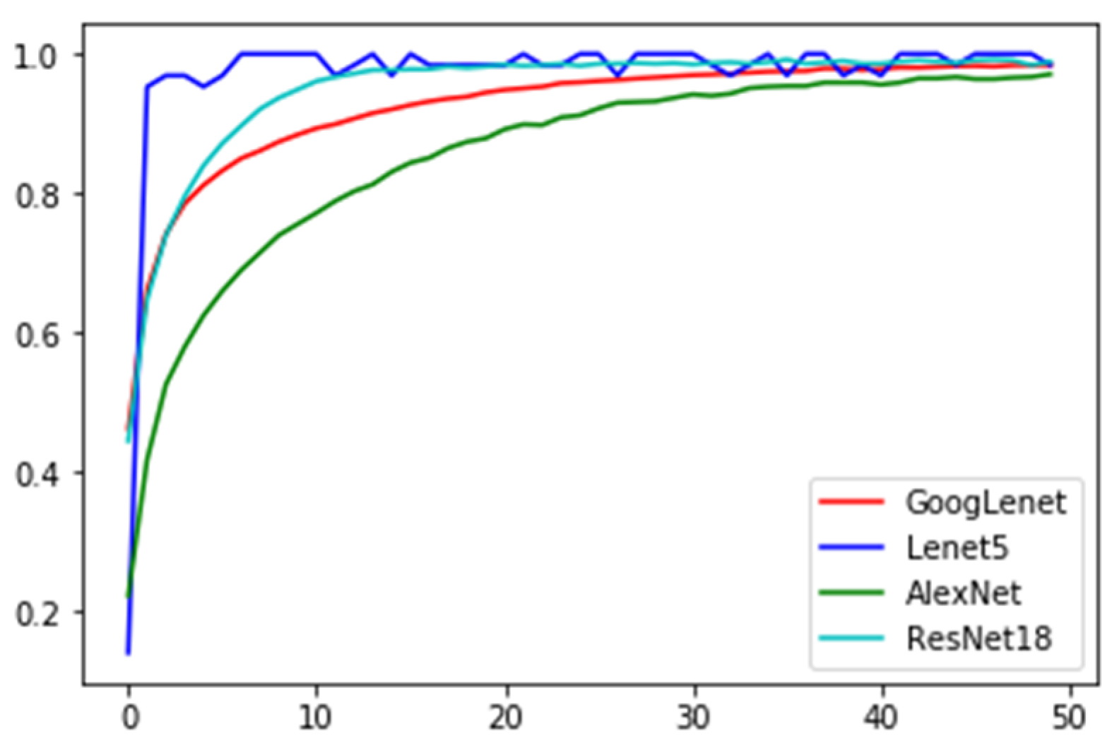
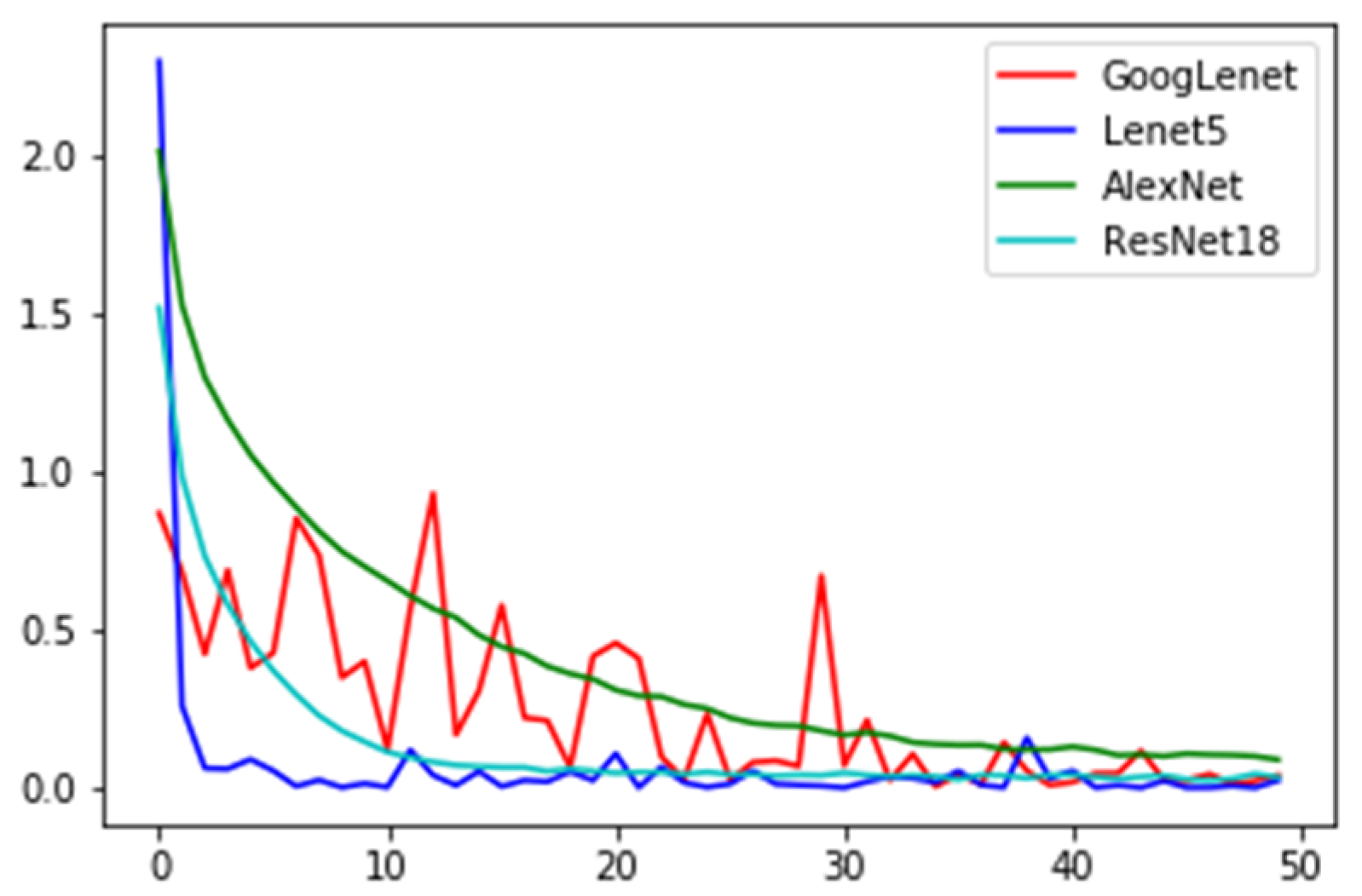
To evaluate the performance of the proposed SAGM, different experiments were conducted on the two image datasets, namely MNIST and CIFAR10, which have different image dimensions and category numbers. MNIST is a dataset of 28 × 28 gray-scale handwritten digits in the range of 0 to 9, containing 60,000 training samples and 10,000 testing samples. CIFAR-10 is a 32 × 32 color image containing 10 categories, with 6000 images per category. One DNN model, namely LeNet5 [44], was pre-trained in the MNIST dataset, while three DNN models, namely ResNet18 [45], AlexNet [46], and GoogLeNet [47], were selected as the CIFAR-10 dataset. For MNIST and CIFAR-10, all training samples were used to train the accuracy of the DNN used in this paper, and all test samples were used to verify the robustness of the DNN.

Moreover, for this DNN model, parameters were consistent with the original framework. All the experiments were carried out on a computer with an Intel Core i-7 CPU and 16 GB RAM. LeNet5 on the MNIST achieved an accuracy of 98.44%, and ResNet18, AlexNet, and GoogLeNet on the Cifar-10 achieved accuracies of 98.90%, 96.46%, and 98.38%, respectively. Furthermore, four attack algorithms, namely FGM [48], PGD, CW, and BMI-FGSM were selected for comparison with our attack algorithm. The curves of training accuracy and loss are shown in Figure 5 and Figure 6, respectively.

Figure 5. Network training accuracy.

Figure 6. Network training loss.

4.2. Measurement

4.2.1. Comparison

In this subsection, comprehensive metrics were used to evaluate different adversarial attack techniques

The attack success rate (ASR) is the ratio of the number of successfully attacked images to all the test images. The larger the value, the lower the accuracy of DNN. The calculation is shown in Equation (21)

$$ASR=\frac{Nu{m}_{success }}{Nu{m}_{total}}$$

(21)

where Num_success is the number of successfully attacked images and Num_total is the number of all the test images. For the MNIST dataset, the ASRs of five attack methods on LeNet5 are presented in Table 1. The results in Table 1 show that the SAGM has the highest value on ASR; therefore, the proposed SAGM has better performance.

Table 1. Attack Success Rate on the MNIST Dataset.

DNN	FGM	PGD	CW	BMI-FGSM	SAGM
LeNet5	49.14%	92.75%	92.00%	99.40%	100.00%

For the CIFAR-10 dataset, the ASRs of five attack methods on ResNet18 and AlexNet are shown in Table 2. PGD achieved a 100% success rate on ResNet18 and the SAGM, but slightly lower than the SAGM on AlexNet. Therefore, the SAGM and BMI-FGSM a have better performance among these attack algorithms.

Table 2. Attack Success Rate on the CIFAR10 Dataset.

DNN	FGM	PGD	CW	BMI-FGSM	SAGM
ResNet18	98.59%	100.00%	95.70%	100.00%	100.00%
AlexNet	92.19%	99.12%	73.86%	100.00%	100.00%

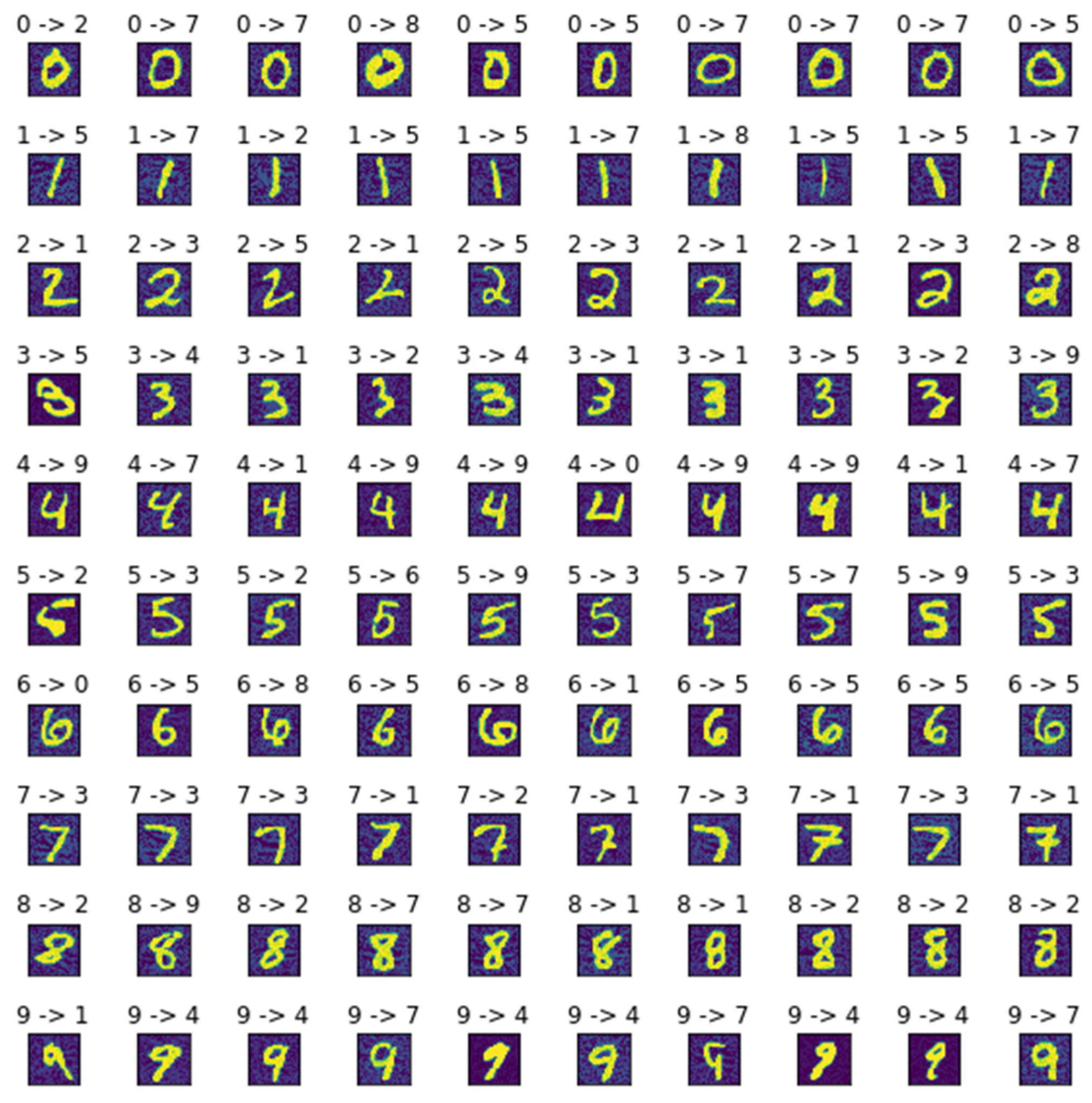
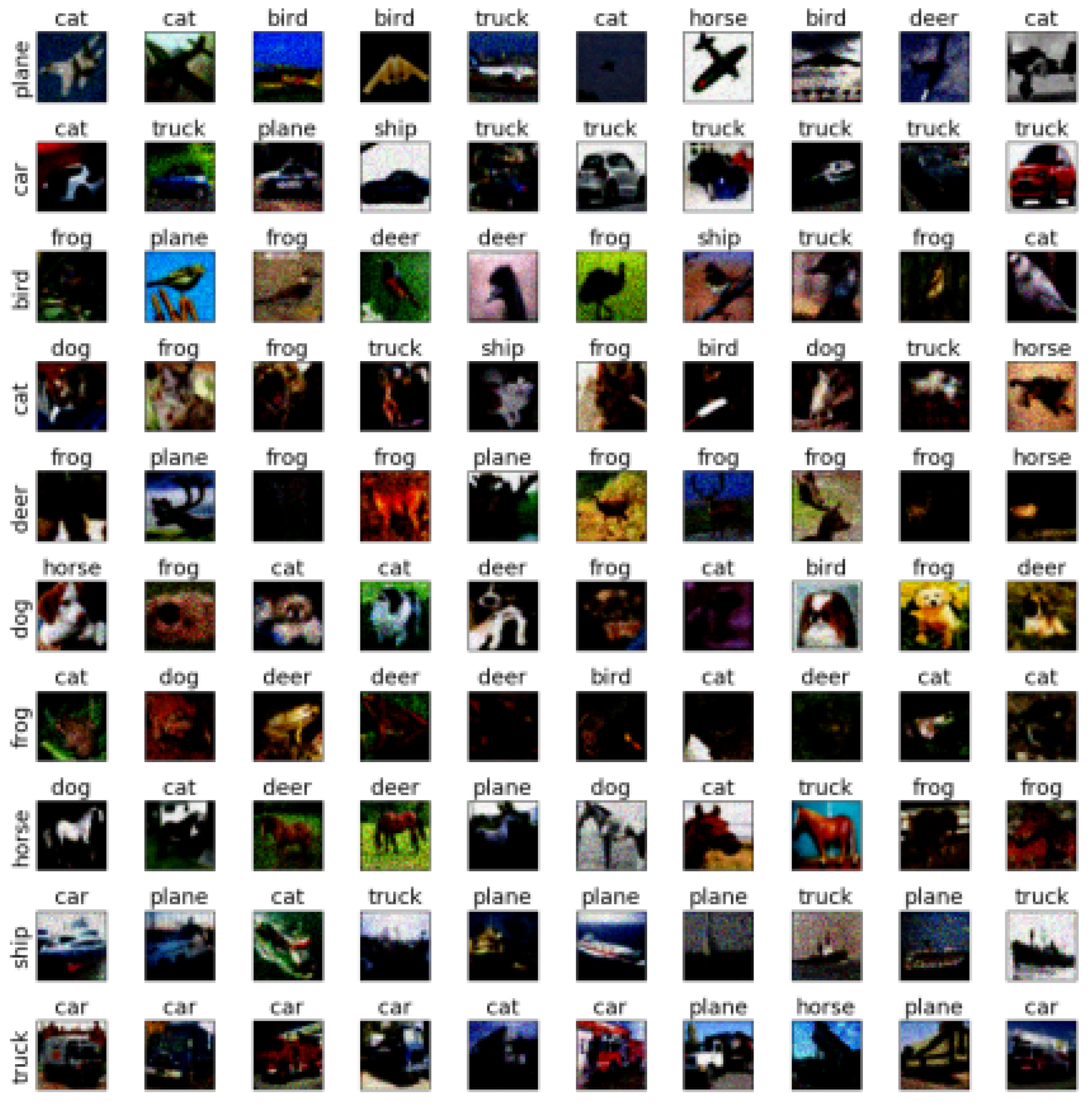
Transferability AEs generated for one ML model can be used to misclassify another model, even if both models have different architecture and training data. This property is called transferability. The adversarial examples of the SAGM for MNIST and Cifar10 are shown in Figure 7 and Figure 8, respectively. The proposed algorithm was found to have a good effect.

Figure 7. The adversarial examples of SAGM for MNIST.

Figure 8. The adversarial examples of SAGM for Cifar10.

Robustness is a metric used to evaluate the flexibility of DNNs to adversarial examples. The model robustness to adversarial perturbations is defined as the following Equation (22).

$$\begin{array}{c}{\Delta }_{adv}\left(x,p\right)=\underset{\delta \in {[0,1]}^n}{min}\parallel \delta {\parallel }_p\\ s.t. p\left(x,t\right)p\left(x+\delta ,t\right)\le 0\end{array}$$

(22)

The robustness of the three DNNs on the three norms is shown in Table 3. The smaller the value, the smaller the distance between the adversarial examples and the real samples. The best mean values are shown in bold. The results show that the samples generated based on the white-box attack have a better adversarial distance than the black-box attack because it utilizes the DNN gradient.

Table 3. Robustness of DNNs.

DNN	Norm	FGM	PGD	CW	BMI-FGSM	SAGM
LeNet5	1	1.61 × 101	2.23 × 101	2.66 × 101	1.40 × 102	1.39 × 102
	2	9.47 × 10	1.32 × 10−1	1.38 × 101	1.230 × 101	1.52 × 101
	Inf	1.43 × 101	1.96 × 101	2.60 × 101	2.03 × 101	3.73 × 10
ResNet18	1	9.70 × 101	5.87 × 101	2.22 × 102	6.16 × 101	1.11 × 102
	2	3.24 × 10	2.18 × 10	1.74 × 101	1.32 × 10	3.34 × 10
	Inf	2.90 × 10−1	2.97 × 10−1	2.54 × 10	2.65 × 10−1	2.41 × 10−1
AlexNet	1	9.18 × 102	5.18 × 102	2.09 × 103	5.85 × 102	1.56 × 103
	2	1.33 × 101	7.66 × 10	5.43 × 101	9.39 × 101	1.57 × 101
	Inf	5.33 × 10−1	3.00 × 10−1	2.53 × 10	8.32 × 10−1	4.10 × 10−1

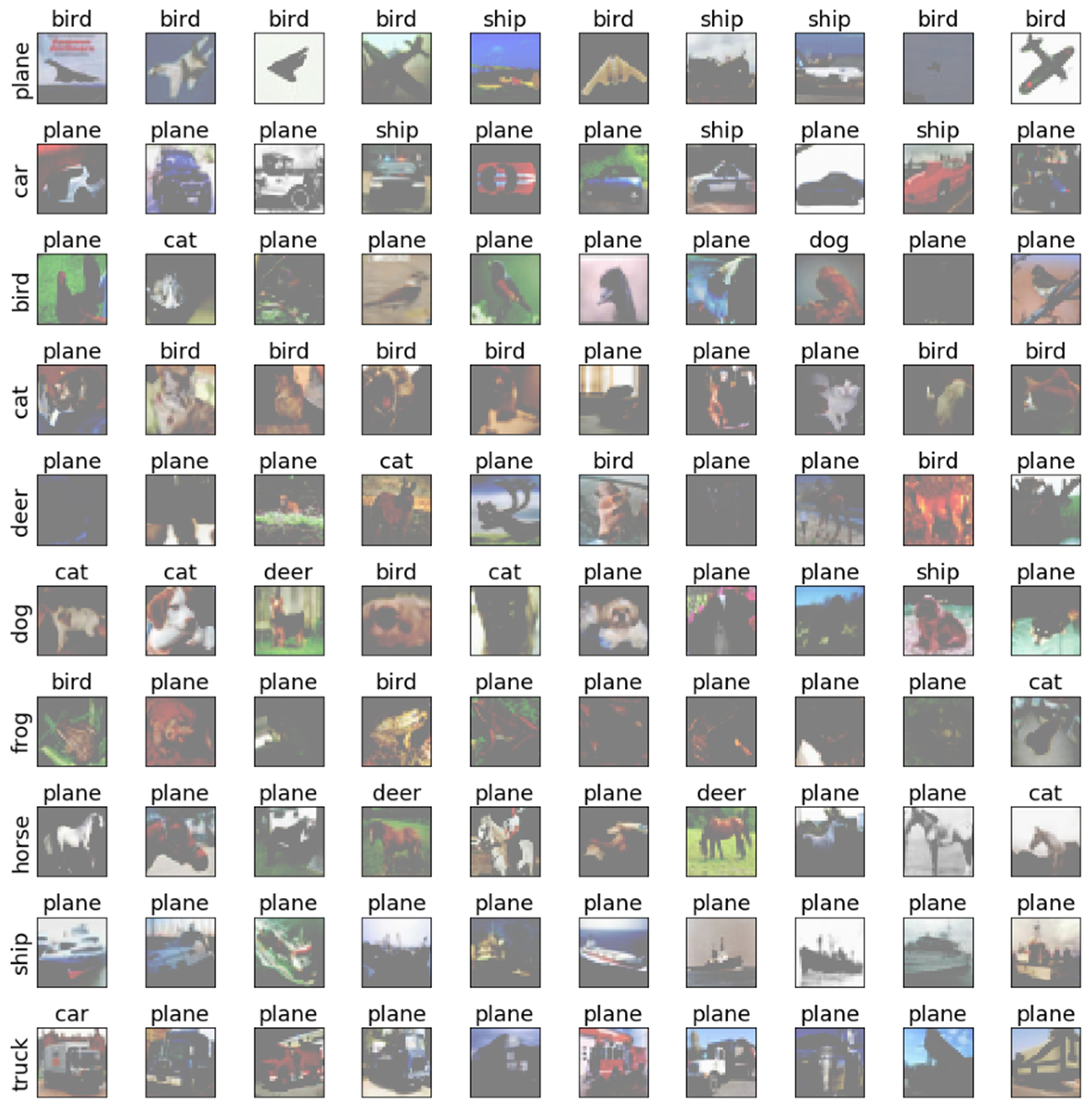
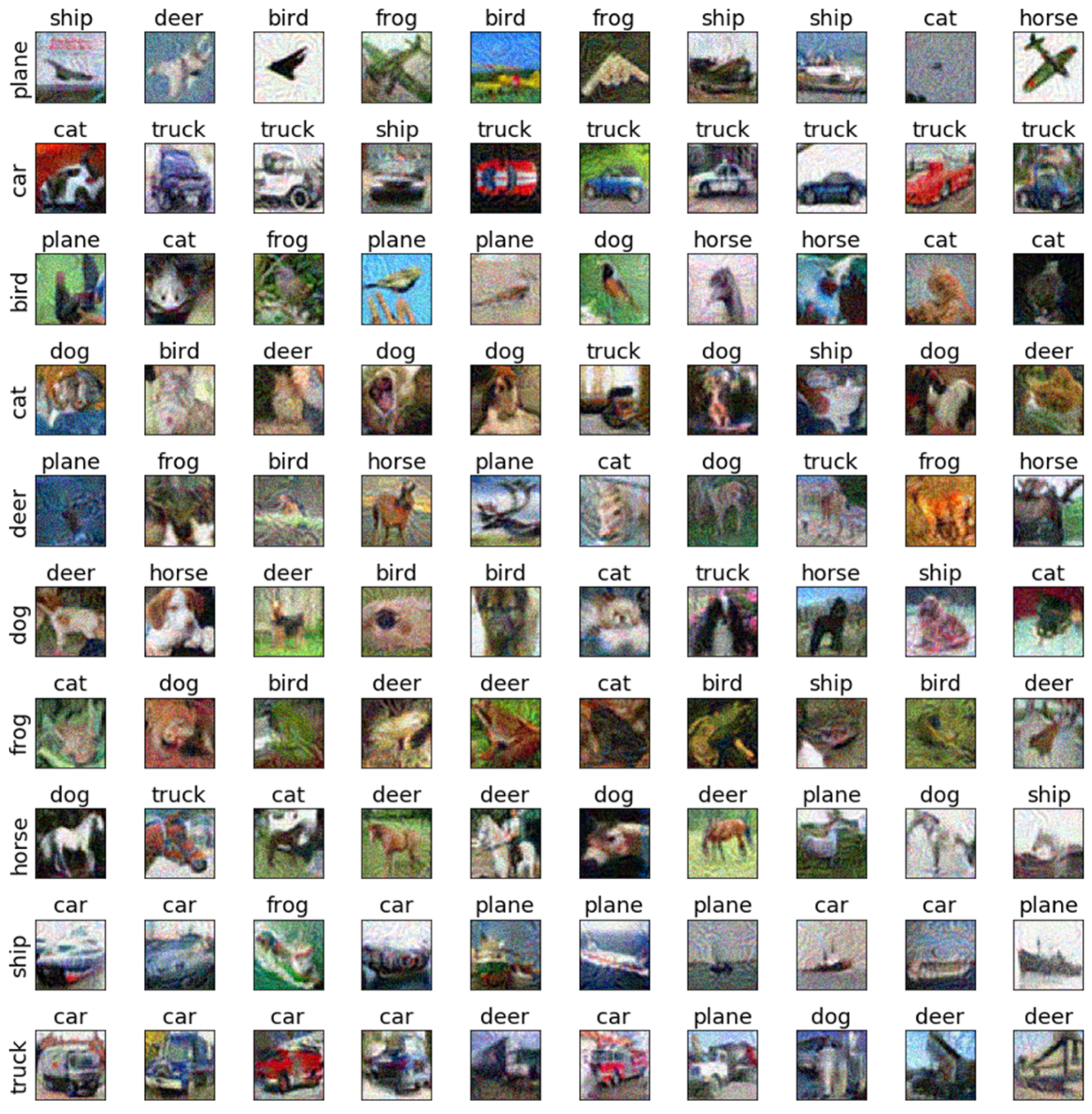
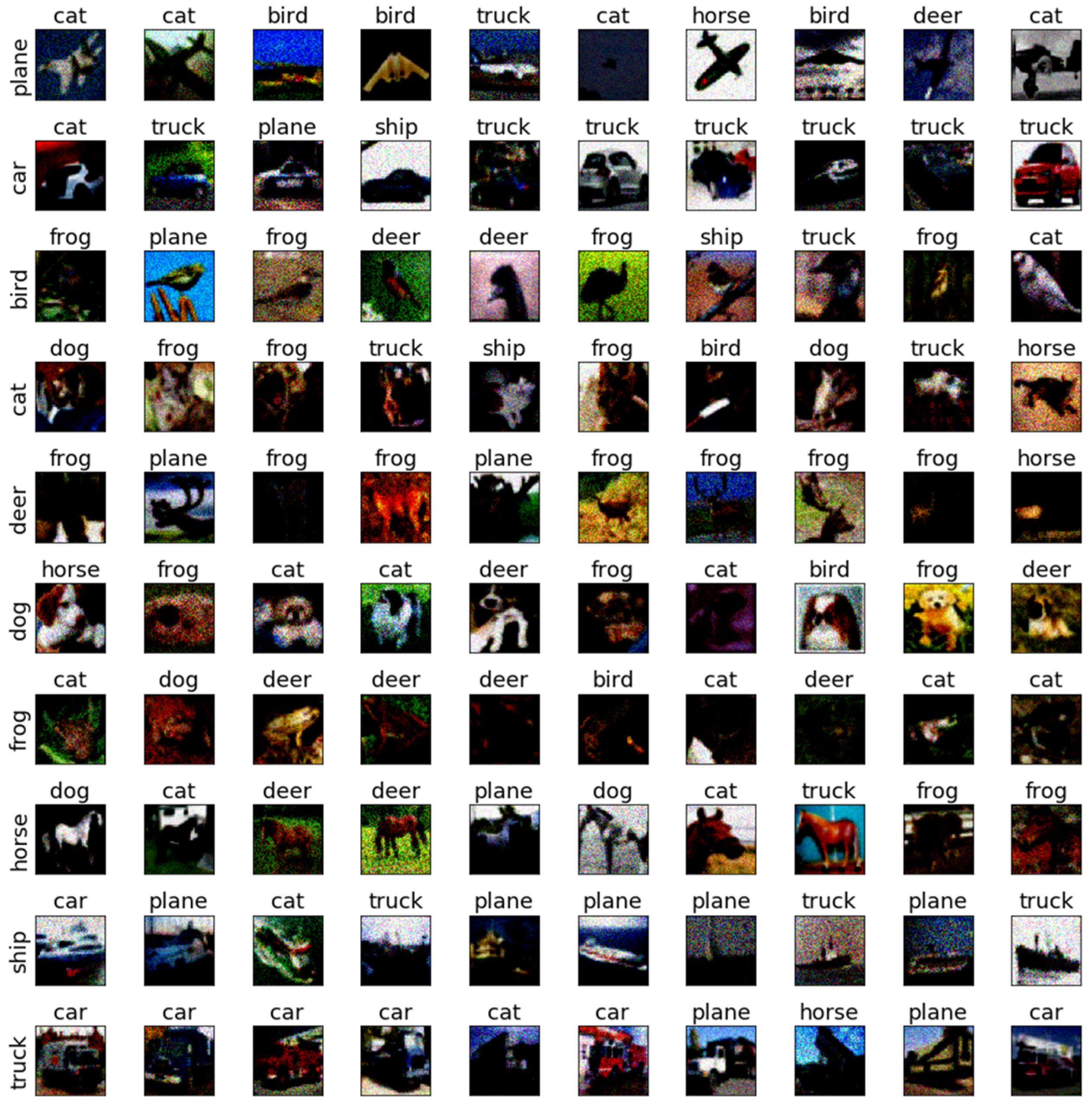
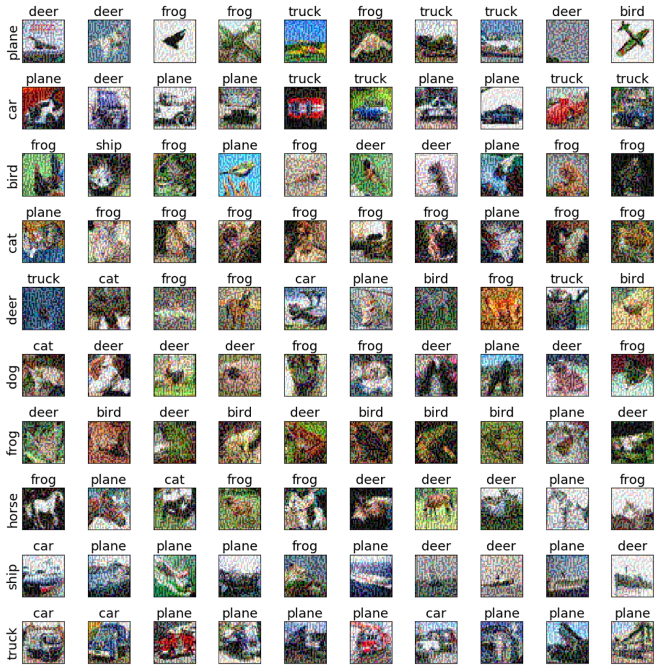
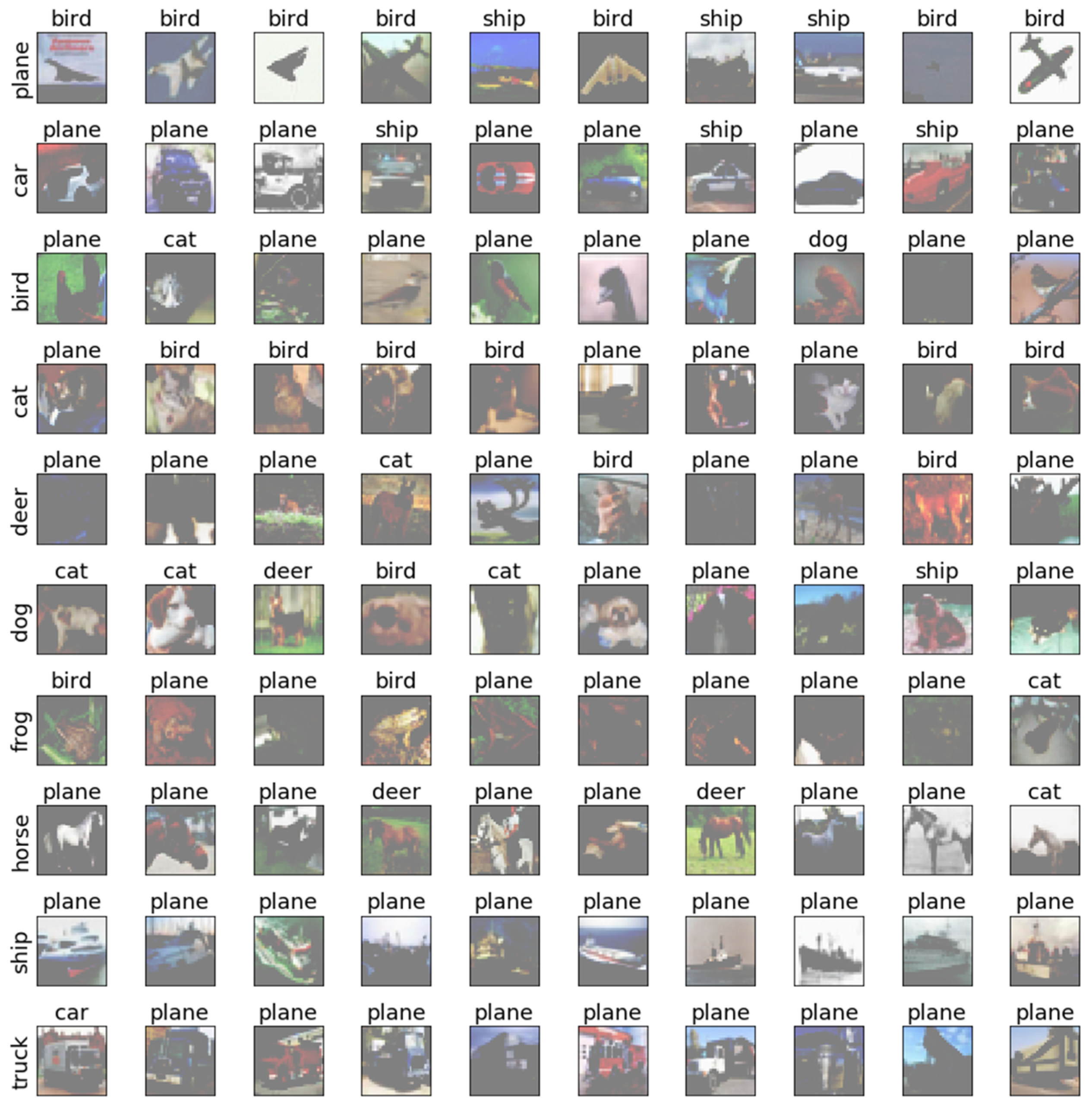
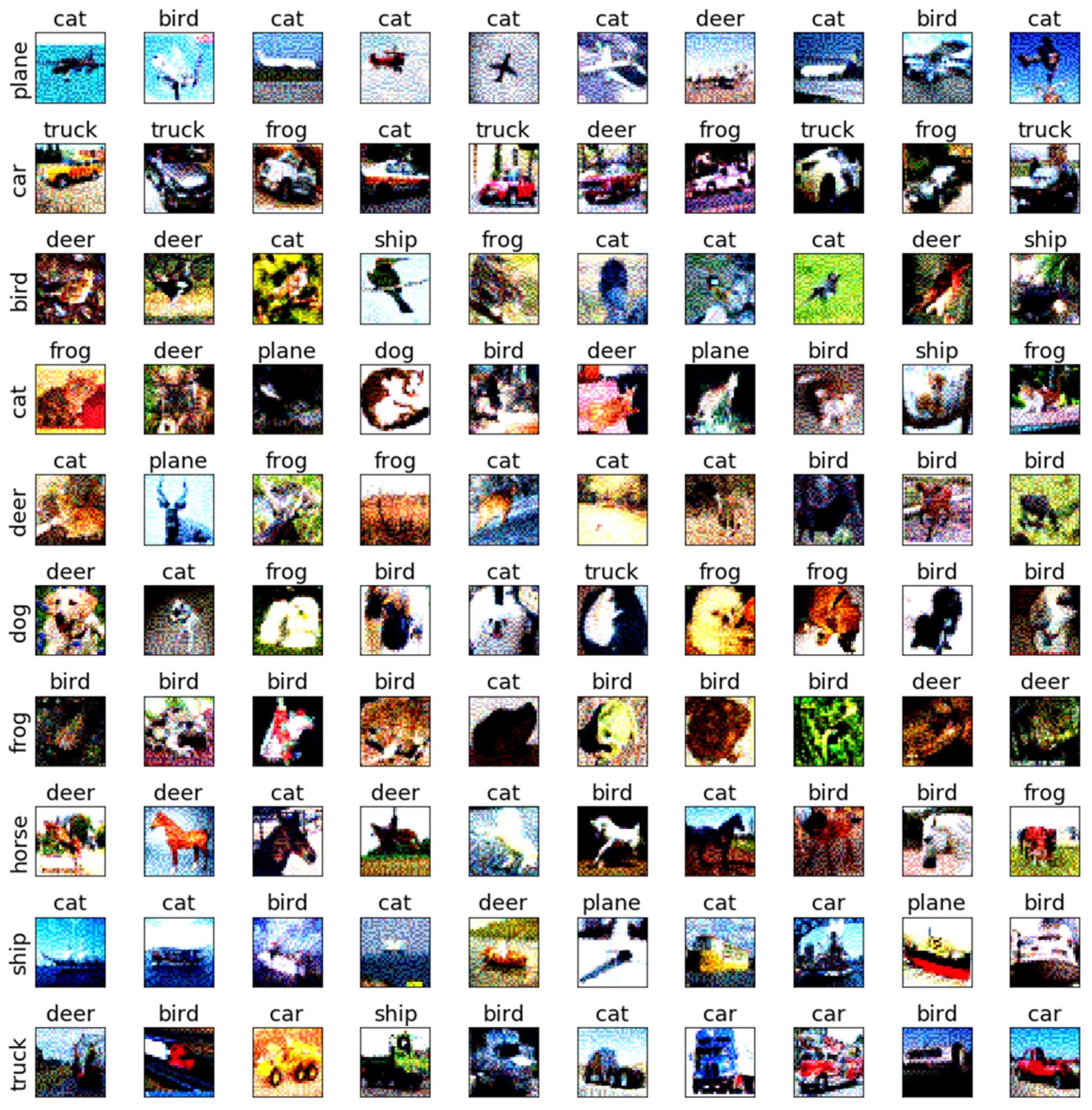
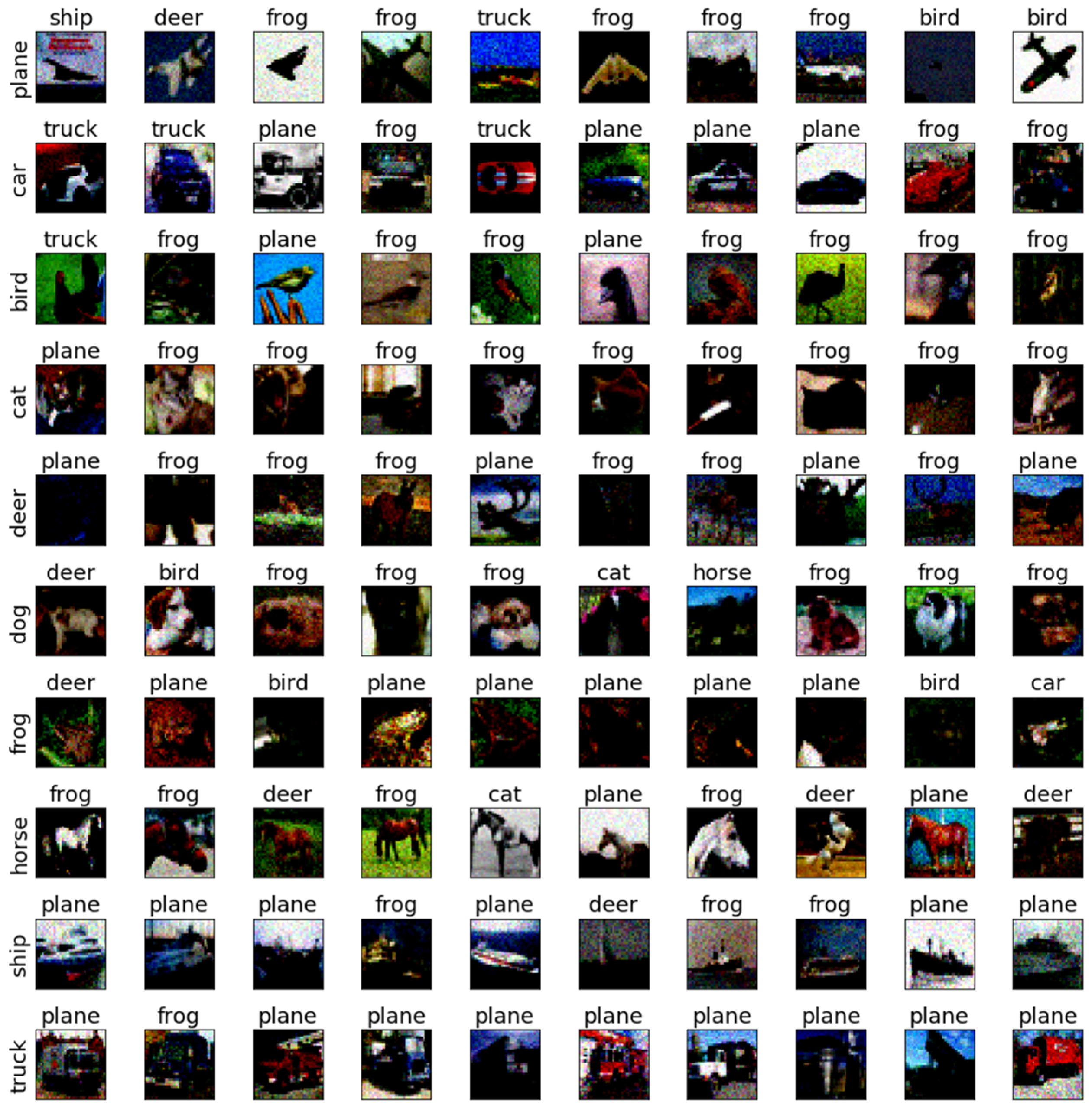
To further discuss the sensitivity of each class of images, we selected the testing samples from the CIFAR-10 dataset on AlexNet and ResNet18 to verify the sensitivity. The adversarial examples are shown in Figure 9, Figure 10, Figure 11, Figure 12, Figure 13, Figure 14, Figure 15, Figure 16, Figure 17 and Figure 18. From these figures, we found that the SAGM algorithm has a better adversarial effect and higher clarity.

Figure 9. The adversarial examples of FGM for Cifar10 and AlexNet.

Figure 10. The adversarial examples of CW for Cifar10 and AlexNet.

Figure 11. The adversarial examples of PGD for Cifar10 and AlexNet.

Figure 12. The adversarial examples of BMI-FGSM for Cifar10 and AlexNet.

Figure 13. The adversarial examples of SAGM for Cifar10 and AlexNet.

Figure 14. The adversarial examples of FGM for Cifar10 and ResNet18.

Figure 15. The adversarial examples of CW for Cifar10 and ResNet18.

Figure 16. The adversarial examples of PGD for Cifar10 and ResNet18.

Figure 17. The adversarial examples of BMI-FGSM for Cifar10 and ResNet18.

Figure 18. The adversarial examples of SAGM for Cifar10 and ResNet18.

Structural similarity (SSIM) measurement, consisting of three comparisons of luminance, contrast, and structure, was proposed to evaluate the similarity between two images. The SSIM between image x and x′ is modeled as Equation (23).

$$SSIM\left(x,x^{\prime }\right)=\frac{1}{m}\sum _{n=1}^m\left[L{\left(x_n,x_n^{\prime }\right)}^{\alpha }C{\left(x_n,x_n^{\prime }\right)}^{\beta }S{\left(x_n,x_n^{\prime }\right)}^{\gamma }\right]$$

(23)

where m is the number of pixels and L, C, and S are the image’s luminance, contrast, and structure, respectively, α = β = γ = 1. The comparison of structural similarity is shown in Table 4, and the best mean values are shown in bold. The results show that CW has a clear advantage on LeNet5 but is almost similar in the other two DNNs.

Table 4. SSIM of DNNs.

DNN	FGM	PGD	CW	BMI-FGSM	SAGM
LeNet5	5.62 × 10−1	7.66 × 10−1	7.94 × 10−2	6.25 × 10−1	5.34 × 10−1
ResNet18	7.92 × 10−1	8.86 × 10−1	2.57 × 10−1	8.63 × 10−1	8.39 × 10−1
AlexNet	5.18 × 10−1	6.68 × 10−1	3.69 × 10−1	6.92 × 10−1	4.47 × 10−1

4.2.2. Effectiveness of Adaptive Step

To verify the effect of the adaptive step, Equation (11) is embedded in FGM and PGD. The effectiveness of adaptive steps is shown in Table 5. The results show that the adaptive step size is beneficial to improve ASR.

Table 5. Effect of Adaptive Steps.

DNN	FGM	FGM-Adaptive	PGD	PGD-Adaptive
LeNet5	49.14%	49.25%	92.75%	92.80%
ResNet18	98.59%	99.62%	100.00%	100.00%
AlexNet	92.19%	93.15%	99.12%	100.00%

4.2.3. Evaluation

To sum up, we compared the SAGM with existing adversarial training algorithms and the results show that the algorithm that we proposed has an excellent performance in attack model evaluation metrics, such as attack success rate, transferability, robustness, sensitivity, and structural similarity (SSIM) measurement. The attack success rate is an important evaluation index of the adversarial training algorithm, which is equivalent to the accuracy of the recognition algorithm, Table 1 and Table 2 show that the SAGM can reach a very high success rate in this index and it can carry out accurate and no-miss attacks. Figure 7 and Figure 8 show the transferability of the SAGM. Table 3 shows the robustness of SAGM compared with other existing algorithms. Figure 9, Figure 10, Figure 11, Figure 12, Figure 13, Figure 14, Figure 15, Figure 16, Figure 17 and Figure 18 show the sensitivity of SAGM, it has a better adversarial effect and higher clarity. Table 4 shows the result of SSIM that the SAGM compared with other existing algorithms.

At the same time, the self-adaptive algorithm is also effective for existing adversarial algorithms. When added to other adversarial algorithms, it can improve the ASK of other algorithms, which is shown in Table 5.

5. Conclusions

In this paper, we proposed a gradient simulation method for the black-box adversarial attack, SAGM, for the score-based generation of adversarial examples. It is very difficult to use adversarial examples to identify and successfully fool DNNs on MNIST and CIFAR10. Two operations, namely the self-adaptive approximated gradient simulation and the momentum gradient-based perturbation sample generation, were proposed to explore the sensitive gradient direction and generate the efficiency perturbation samples to attack DNNs. The extensive experiments showed that the SAGM achieves excellent performance comparable to other attack algorithms in success rate, perturbation distance, and transferability. In the future, the effect of this study will be a focus on improving the evaluation model to generate more efficient adversarial examples to achieve a balance between adversarial examples and the human visual system. In addition, we believe that some sensitive pixels can be explored to perturb partial pixels of clean images to improve the robustness of adversarial examples. Furthermore, another direction is the application of other intelligent optimization algorithms to adversarial attacks.

References

1. Junior, F.E.F.; Yen, G.G. Particle swarm optimization of deep neural networks architectures for image classification. Swarm Evol. Comput. 2019, 49, 62–74. [Google Scholar] [CrossRef]
2. Cococcioni, M.; Rossi, F.; Ruffaldi, E.; Saponara, S.; Dupont de Dinechin, B. Novel arithmetics in deep neural networks signal processing for autonomous driving: Challenges and opportunities. IEEE Signal Process. Mag. 2020, 38, 97–110. [Google Scholar] [CrossRef]
3. Janai, J.; Güney, F.; Behl, A.; Geiger, A. Computer vision for autonomous vehicles: Problems, datasets and state of the art. Found. Trends® Comput. Graph. Vis. 2020, 12, 1–308. [Google Scholar] [CrossRef]
4. Lee, S.; Song, W.; Jana, S.; Cha, M.; Son, S. Evaluating the robustness of trigger set-based watermarks embedded in deep neural networks. IEEE Trans. Dependable Secur. Computing 2022, 1–15. [Google Scholar] [CrossRef]
5. Ren, H.; Huang, T.; Yan, H. Adversarial examples: Attacks and defenses in the physical world. Int. J. Mach. Learn. Cybern. 2021, 12, 3325–3336. [Google Scholar] [CrossRef]
6. Shen, J.; Robertson, N. Bbas: Towards large scale effective ensemble adversarial attacks against deep neural network learning. Inf. Sci. 2021, 569, 469–478. [Google Scholar] [CrossRef]
7. Garg, S.; Ramakrishnan, G. Bae: Bert-based adversarial examples for text classification. In Proceedings of the 2020 Conference on Empirical Methods in Natural Language Processing (EMNLP), Punta Cana, Dominican Republic, 8 May 2020. [Google Scholar] [CrossRef]
8. Rahman, A.; Hossain, M.S.; Alrajeh, N.A.; Alsolami, F. Adversarial examplesłsecurity threats to COVID-19 deep learning systems in medical iot devices. IEEE Internet Things J. 2020, 8, 9603–9610. [Google Scholar] [CrossRef]
9. Finlayson, S.G.; Bowers, J.D.; Ito, J.J.; Zittrain, L.; Beam, A.L.; Kohane, I.S. Adversarial attacks on medical machine learning. Science 2019, 363, 1287–1289. [Google Scholar] [CrossRef]
10. Prinz, K.; Flexer, A.; Widmer, G. On end-to-end white-box adversarial attacks in music information retrieval. Trans. Int. Soc. Music. Inf. Retr. 2021, 4, 93–104. [Google Scholar] [CrossRef]
11. Guo, C.; Gardner, J.; You, Y.; Wilson, A.G.; Weinberger, K. Simple black-box adversarial attacks. In Proceedings of the 36th International Conference on Machine Learning, Long Beach, CA, USA, 9–15 June 2019; pp. 2484–2493. [Google Scholar] [CrossRef]
12. Wang, Y.; Tan, Y.; Zhang, W.; Zhao, Y.; Kuang, X. An adversarial attack on dnn-based black-box object detectors. J. Netw. Comput. Appl. 2020, 161, 102634. [Google Scholar] [CrossRef]
13. Goodfellow, I.J.; Shlens, J.; Szegedy, C. Explaining and harnessing adversarial examples. arXiv 2014, arXiv:1412.6572. [Google Scholar] [CrossRef]
14. Liu, S.; Chen, P.Y.; Kailkhura, B.; Zhang, G.; Hero, A.; Varshney, P.K. A primer on zeroth-order optimization in signal processing and machine learning: Principals, recent advances, and applications. IEEE Signal Process. Mag. 2020, 37, 43–54. [Google Scholar] [CrossRef]
15. Cai, X.; Zhao, H.; Shang, S.; Zhou, Y.; Deng, W.; Chen, H.; Deng, W. An improved quantum-inspired cooperative co-evolution algorithm with muli-strategy and its application. Expert Syst. Appl. 2021, 171, 114629. [Google Scholar] [CrossRef]
16. Mohammadi, H.; Soltanolkotabi, M.; Jovanović, M.R. On the linear convergence of random search for discrete-time LQR. IEEE Control. Syst. Lett. 2020, 5, 989–994. [Google Scholar] [CrossRef]
17. LeCun, Y. The Mnist Database of Handwritten Digits. 1998. Available online: http://yann.lecun.com/exdb/mnist/ (accessed on 20 September 2018).
18. Hinton, G.E. Training products of experts by minimizing contrastive divergence. Neural Comput. 2002, 14, 1771–1800. [Google Scholar] [CrossRef] [PubMed]
19. Kumar, B.; Dikshit, O.; Gupta, A.; Singh, M.K. Feature extraction for hyperspectral image classification: A review. Int. J. Remote Sens. 2020, 41, 6248–6287. [Google Scholar] [CrossRef]
20. Kurakin, A.; Goodfellow, I.J.; Bengio, S. Adversarial examples in the physical world. In Artificial Intelligence Safety and Security; Chapman Hall/CRC: Boca Raton, FL, USA, 2018; pp. 99–112. [Google Scholar] [CrossRef]
21. Madry, A.; Makelov, A.; Schmidt, L.; Tsipras, D.; Vladu, A. Towards deep learning models resistant to adversarial attacks. Stat 2017, 1050, 9. [Google Scholar] [CrossRef]
22. Dong, Y.; Liao, F.; Pang, T.; Su, H.; Zhu, J.; Hu, X.; Li, J. Boosting adversarial attacks with momentum. In Proceedings of the IEEE Conference on Computer Vision and Pattern Recognition, Salt Lake City, UT, USA, 18–23 June 2018; pp. 9185–9193. [Google Scholar] [CrossRef]
23. Carlini, N.; Wagner, D. Towards evaluating the robustness of neural networks. In Proceedings of the 2017 IEEE Symposium on Security and Privacy (sp). IEEE, San Jose, CA, USA, 22–26 May 2017; pp. 39–57. [Google Scholar] [CrossRef]
24. Chen, P.Y.; Zhang, H.; Sharma, Y.; Yi, J.; Hsieh, C.J. Zoo: Zeroth order optimization based black-box attacks to deep neural networks without training substitute models. In Proceedings of the 10th ACM Workshop on Artificial Intelligence and Security, Dallas, TX, USA, 3 November 2017; pp. 15–26. [Google Scholar] [CrossRef]
25. Su, J.; Vargas, D.V.; Sakurai, K. One pixel attack for fooling deep neural networks. IEEE Trans. Evol. Computation 2019, 23, 828–841. [Google Scholar] [CrossRef]
26. Lin, J.; Xu, L.; Liu, Y.; Zhang, X. Black-box adversarial sample generation based on differential evolution. J. Syst. Softw. 2020, 170, 110767. [Google Scholar] [CrossRef]
27. Li, C.; Wang, H.; Zhang, J.; Yao, W.; Jiang, T. An approximated gradient sign method using differential evolution for black-box adversarial attack. IEEE Trans. Evol. Comput. 2022, 26, 976–990. [Google Scholar] [CrossRef]
28. Storn, R.; Price, K. Differential evolution–a simple and efficient heuristic for global optimization over continuous spaces. J. Glob. Optim. 1997, 11, 341–359. [Google Scholar] [CrossRef]
29. Xu, Z.; Han, G.; Liu, L.; Martínez-García, M.; Wang, Z. Multi-energy scheduling of an industrial integrated energy system by reinforcement learning-based differential evolution. IEEE Trans. Green Commun. Netw. 2021, 5, 1077–1090. [Google Scholar] [CrossRef]
30. Jana, R.K.; Ghosh, I.; Das, D. A differential evolution-based regression framework for forecasting Bitcoin price. Ann. Oper. Res. 2021, 306, 295–320. [Google Scholar] [CrossRef] [PubMed]
31. Njock, P.G.A.; Shen, S.L.; Zhou, A.; Modoni, G. Artificial neural network optimized by differential evolution for predicting diameters of jet grouted columns. J. Rock Mech. Geotech. Eng. 2021, 13, 1500–1512. [Google Scholar] [CrossRef]
32. Luo, G.; Zou, L.; Wang, Z.; Lv, C.; Ou, J.; Huang, Y. A novel kinematic parameters calibration method for industrial robot based on Levenberg-Marquardt and Differential Evolution hybrid algorithm. Robot. Comput. Integr. Manuf. 2021, 71, 102165. [Google Scholar] [CrossRef]
33. Sun, Y.; Song, C.; Yu, S.; Liu, Y.; Pan, H.; Zeng, P. Energy-efficient task offloading based on differential evolution in edge computing system with energy harvesting. IEEE Access 2021, 9, 16383–16391. [Google Scholar] [CrossRef]
34. Singh, D.; Kaur, M.; Jabarulla, M.Y.; Kumar, V.; Lee, H.N. Evolving fusion-based visibility restoration model for hazy remote sensing images using dynamic differential evolution. IEEE Trans. Geosci. Remote Sens. 2022, 60, 1–14. [Google Scholar] [CrossRef]
35. Biswas, S.; Manicka, S.; Hoel, E.; Levin, M. Gene regulatory networks exhibit several kinds of memory: Quantification of memory in biological and random transcriptional networks. iScience 2021, 24, 102131. [Google Scholar] [CrossRef]
36. Tan, X.; Lee, H.; Shin, S.Y. Cooperative Coevolution Differential Evolution Based on Spark for Large-Scale Optimization Problems. J. Inf. Commun. Converg. Eng. 2021, 19, 155–160. [Google Scholar] [CrossRef]
37. Pant, M.; Zaheer, H.; Garcia-Hernandez, L.; Abraham, A. Differential Evolution: A review of more than two decades of research. Eng. Appl. Artif. Intell. 2020, 90, 103479. [Google Scholar] [CrossRef]
38. Baioletti, M.; Di Bari, G.; Milani, A.; Poggioni, V. Differential evolution for neural networks optimization. Mathematics 2020, 8, 69. [Google Scholar] [CrossRef]
39. Zhang, J.; Sanderson, A.C. JADE: Adaptive differential evolution with optional external archive. IEEE Trans. Evol. Comput. 2009, 13, 945–958. [Google Scholar] [CrossRef]
40. Tan, X.; Shin, S.Y.; Shin, K.S.; Wang, G. Multi-Population Differential Evolution Algorithm with Uniform Local Search. Appl. Sci. 2022, 12, 8087. [Google Scholar] [CrossRef]
41. Georgioudakis, M.; Plevris, V. A comparative study of differential evolution variants in constrained structural optimization. Front. Built Environ. 2020, 6, 102. [Google Scholar] [CrossRef]
42. Ronkkonen, J.; Kukkonen, S.; Price, K.V. Real-parameter optimization with differential evolution. IEEE Congr. Evol. Comput. 2005, 1, 506–513. [Google Scholar] [CrossRef]
43. Ali, M.M.; Torn, A. Population set-based global optimization algorithms: Some modifications and numerical studies. Comput. Oper. Res. 2004, 31, 1703–1725. [Google Scholar] [CrossRef]
44. LeCun, Y.; Jackel, L.; Bottou, L.; Brunot, A.; Cortes, C.; Denker, J.; Drucker, H.; Guyon, I.; Muller, U.; Sackinger, E.; et al. Comparison of learning algorithms for handwritten digit recognition. Int. Conf. Artif. Neural Netw. 1995, 60, 53–60. [Google Scholar]
45. He, K.; Zhang, X.; Ren, S.; Sun, J. Deep residual learning for image recognition. In Proceedings of the IEEE Conference on Computer Vision and Pattern Recognition, Las Vegas, NV, USA, 27–30 June 2016; pp. 770–778. [Google Scholar] [CrossRef]
46. Krizhevsky, A.; Sutskever, I.; Hinton, G.E. Imagenet classification with deep convolutional neural networks. Commun. ACM 2017, 60, 84–90. [Google Scholar] [CrossRef]
47. Szegedy, C.; Liu, W.; Jia, Y.; Sermanet, P.; Reed, S.; Anguelov, D.; Erhan, D.; Vanhoucke, V.; Rabinovich, A. Going deeper with convolutions. In Proceedings of the IEEE Conference on Computer Vision and Pattern Recognition, Boston, MA, USA, 7–12 June 2015; pp. 1–9. [Google Scholar] [CrossRef]
48. Kurakin, A.; Goodfellow, I.; Bengio, S. Adversarial machine learning at scale. arXiv 2016, arXiv:1611.01236. [Google Scholar] [CrossRef]
Disclaimer/Publisher’s Note: The statements, opinions and data contained in all publications are solely those of the individual author(s) and contributor(s) and not of MDPI and/or the editor(s). MDPI and/or the editor(s) disclaim responsibility for any injury to people or property resulting from any ideas, methods, instructions or products referred to in the content.
Article Metrics
Citations
Article Access Statistics
Multiple requests from the same IP address are counted as one view.