Cuckoo Coupled Improved Grey Wolf Algorithm for PID Parameter Tuning

Abstract

In today’s automation control systems, the PID controller, as a core technology, is widely used to maintain the system output near the set value. However, in some complex control environments, such as the application of ball screw-driven rotating motors, traditional PID parameter adjustment methods may not meet the requirements of high precision, high performance, and fast response time of the system, making it difficult to ensure the stability and production efficiency of the mechanical system. Therefore, this paper proposes a cuckoo search optimisation coupled with an improved grey wolf optimisation (CSO_IGWO) algorithm to tune PID controller parameters, aiming at resolving the problems of the traditional grey wolf optimisation (GWO) algorithm, such as slow optimisation speed, weak exploitation ability, and ease of falling into a locally optimal solution. First, the tent chaotic mapping method is used to initialise the population instead of using random initialization to enrich the diversity of individuals in the population. Second, the value of the control parameter is adjusted by the nonlinear decline method to balance the exploration and development capacity of the population. Finally, inspired by the cuckoo search optimisation (CSO) algorithm, the Levy flight strategy is introduced to update the position equation so that grey wolf individuals are enabled to make a big jump to expand the search area and not easily fall into local optimisation. To verify the effectiveness of the algorithm, this study first verifies the superiority of the improved algorithm with eight benchmark test functions. Then, comparing this method with the other two improved grey wolf algorithms, it can be seen that this method increases the average and standard deviation by an order of magnitude and effectively improves the global optimal search ability and convergence speed. Finally, in the experimental section, three parameter tuning methods were compared from four aspects: overshoot, steady-state time, rise time, and steady-state error, using the ball screw motor as the control object. In terms of overall dynamic performance, the method proposed in this article is superior to the other three parameter tuning methods.

1. Introduction

The PID control algorithm has a simple principle, flexible application, and a wide application range. This algorithm can achieve a certain control effect without knowledge of the specific model of the controlled system. However, the key to the effectiveness of the PID controller is the accuracy of the parameters; hence, the tuning of the PID controller parameters is particularly important. During nearly 100 years of research on PID controllers, many methods for tuning and optimising PID control parameters have been proposed [1,2,3], including empirical trial and error, Ziegle–Nichols, and theoretical design methods, which are relatively old traditional parameter tuning methods; they have the disadvantages of heavy workload and strong blindness [4]. However, in an actual industrial system, the controlled system generally has the characteristics of nonlinearity, time variation, and time delay. When there are many performance objectives for the controlled object, coordinating each performance objective with the turning parameters is difficult, and the traditional and old parameter optimisation methods are no longer suitable for the requirements of current control systems. Therefore, intelligent optimisation algorithms have emerged as new parameter optimisation methods for a new generation of controllers.

For example, the genetic algorithm, a commonly used optimisation algorithm, has been applied to the optimisation of PID control parameters. In [5], the hydraulic servo system uses a genetic algorithm to search for the optimal PID controller gain to achieve accurate control of the displacement of the valve-controlled hydraulic cylinder in the system. Xiao et al. [6] proposed an improved genetic algorithm and verified it using eight test functions. The results showed that the probability of convergence to the optimal value was improved, and it was verified on a beer-filling machine system. In addition, the particle swarm optimisation (PSO) algorithm, an old optimisation algorithm, was proposed by Kennedy and Eberhart in 1995 and is also widely used for parameter tuning in its algorithm application. Javier et al. [7] used a multi-objective particle swarm optimisation algorithm to tune PID parameters and proposed an evaluation system in the virtual model that focused on the evaluation of the establishment time, overshoot, steady-state error, and control performance. Finally, it proves the superiority of the method in UAV experiments. Based on predecessors, Ye et al. [8] proposed an improved PSO to tune the PID parameters of the nonlinear hydraulic system, thereby improving the search efficiency and exploration ability. However, the above controller parameter optimisation methods have problems such as premature convergence, slow convergence speed, and cumbersome parameter setting. In 2014, Mirjalili et al. [9] proposed the grey wolf optimisation (GWO) algorithm, which mainly simulates the social class and hunting process of grey wolves. Compared with other intelligent optimisation algorithms, GWO has the advantages of a simple structure, few setting parameters, easy realisation, etc. However, similar to other algorithms based on random populations, such as the genetic algorithm [10] and PSO [11], GWO also faces some challenging problems with the increase in the search space dimension. To improve the performance of the GWO algorithm, many studies have proposed ideas for improvement. For example, Rodrigues et al. [12] and others introduced a new operator to the traditional GWO algorithm for hierarchical transformations. The biggest change in their approach from the original GWO is based on the use of fuzzy logic. Kumar et al. [13] proposed two new concepts of prey weight and astrophysics to improve the position update equation of the GWO algorithm. Haidari et al. [14] combined the Levy flight strategy with a greedy selection strategy and hunting equation and carried out experimental verification on 29 test platforms.

With rapid technological advancements, there has been a pressing demand to fine-tune or optimise processes, software, models, or structures to achieve the highest levels of accuracy and efficiency. Compared to experimentation or simulation, optimization algorithms are preferred due to their broader problem solving capabilities, reducing the need for human intervention. In recent years, integrating natural phenomena into algorithm design has significantly enhanced the efficiency of optimizing complex, multidimensional, non-continuous, non-differentiable, and noisy problem search spaces [15,16,17]. The function of a PID controller is to determine the system’s steady-state error based on the actual setpoint and output values. By adjusting the values of the proportional, integral, and derivative parameters, the PID controller’s control effect on the controlled object can be modified. Therefore, in many cases, adjusting PID controller parameters is indispensable in control systems as it constitutes a critical method for achieving control objectives. When dealing with complex control objects exhibiting nonlinear and time-delay characteristics, manual computation is laborious, time-consuming, and prone to parameter errors. Even after fine-tuning the parameter control system, achieving the desired control effect is nearly impossible. For such complex control objects, many scholars have applied swarm intelligence algorithms to optimise PID parameters.

Zhao Z.Q. et al. [18] proposed a new evolutionary algorithm based on a quasi-affine transformation, significantly enhancing its global search capability. This quadruplet algorithm was demonstrated to exhibit superior parameter tuning capabilities by comparing simulation results with PID parameter tuning methods based on particle swarm optimisation and the standard quadruplet algorithm. However, the enhancement in the algorithm’s global search capability is established upon reducing the initial population size. This implies that a smaller population could result in incomplete exploration, thereby diminishing the accuracy of parameter tuning. Soleimani Amiri M. et al. [19] and colleagues applied swarm intelligence optimisation algorithms to trajectory control in a complex multi-joint structure. They used the gains initialised by the Ziegler–Nichols method in a PID controller as inputs for the Adaptive Particle Swarm Optimisation (APSO) algorithm to minimise trajectory errors in the multi-joint structure. However, this method requires multiple repetitions of the optimisation process when facing new trajectories. Caponetto R [20] et al. extended the conventional integer-order PID controller to a non-integer order PID controller, and the proposal of this new type of PID controller provides a more flexible tuning scheme for subsequent parameter tuning strategies. Altintas G. et al. [21] proposed two methods, the Genetic Algorithm (GA) and the Big Bang Big Crunch (BBBC) algorithm, for parameter tuning of integer-order PID and fractional-order PID and applied them to the magnetic suspension system. The results showed that the performance of the fractional order controller based on BBBC was better than that of the integer order controller optimised by GA. To enhance the dynamic performance and robustness of micro gas turbine control systems, Yang R [22] et al. proposed a fractional-order PID controller algorithm based on the optimally improved Particle Swarm Optimisation (PSO) and Cuckoo Search (CS) algorithms. Compared to traditional optimisation methods, this approach exhibits superior convergence speed and precision, aiming to improve the control of micro gas turbines for better dynamic performance and robustness.

The problems that the above methods can deal with are relatively limited. Therefore, this paper proposes a cuckoo search optimisation coupled with an improved grey wolf optimisation (CSO_IGWO) algorithm, which mainly uses tent mapping to initialise the population and increase the diversity of the population. A nonlinear control parameter strategy is used to enhance the ability to balance the local and global search, and finally, the idea of the Lévy flight strategy in the CSO algorithm is introduced to improve the location update formula of grey wolf to avoid the premature stagnation of population optimisation.

To sum up, this paper designs a CSO_IGWO algorithm and takes the servo motor system as the controlled object to conduct PID control parameter tuning research. The rest of this paper is arranged as follows: Section 2 outlines the basic GWO algorithm; Section 3 proposes an improved GWO algorithm; and Section 4 presents the mathematical model of the servo motor and conducts numerical data experiments and simulation analysis to prove the effectiveness of the proposed method. Finally, the full text of this paper is summarised in Section 5.

2. Traditional GWO Algorithm

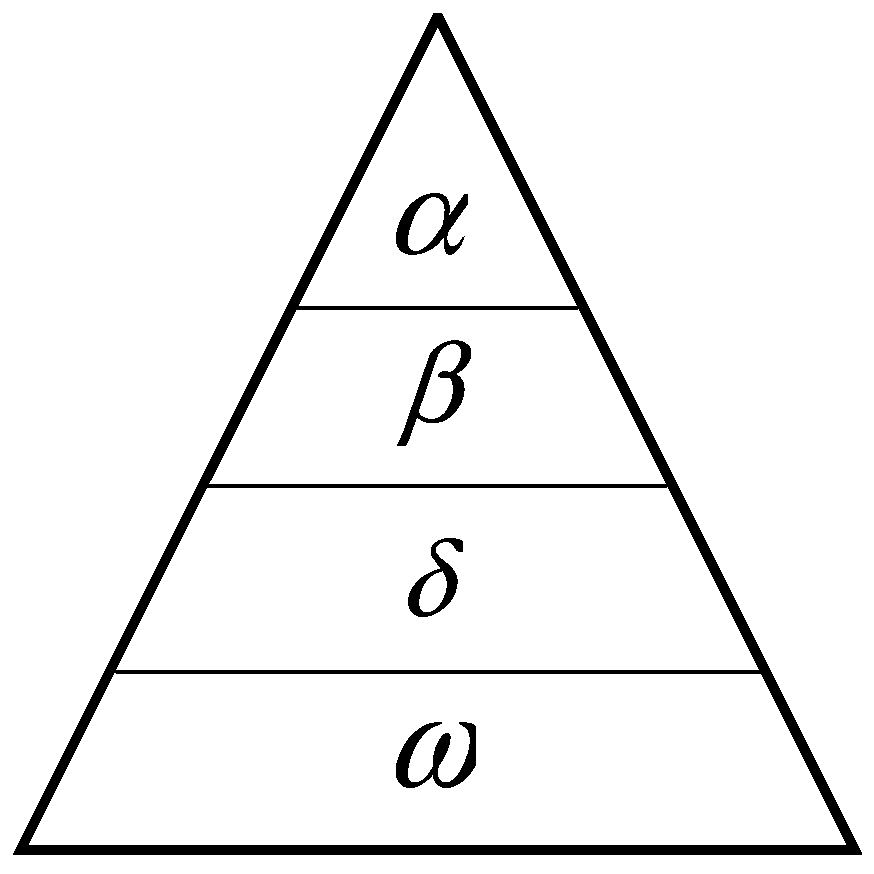
2.1. Social Class of the Grey Wolf

The GWO algorithm is a typical swarm intelligence algorithm inspired by the leadership level and hunting mechanism of grey wolves in nature. The hierarchical distribution structure of the individuals in the traditional GWO algorithm is shown in Figure 1. The entire grey wolf group is divided into four different grey wolf levels. The first social level is the alpha ($\alpha$) wolf, which is the leader of the group and is mainly responsible for making decisions on activities such as predation, roosting, and rest time. The second level of social hierarchy is the beta ($\beta$) wolf, whose role is to help the $\alpha$ wolf make decisions. After the $\alpha$ wolf dies or becomes old, the $\beta$ wolf will become the most suitable candidate to be the $\alpha$ wolf. The third level in the social hierarchy is the delta ($\delta$) wolf, which is subordinate to the $\alpha$ and $\beta$ wolves. The fourth level in the social hierarchy is the omega ($\omega$) wolf, which usually needs to obey wolves at other social levels and ranks lowest in this hierarchy.

2.2. Mathematical Model of the Traditional GWO Algorithm

The core idea of the grey wolf algorithm is to consider $\alpha$, $\beta$, and $\delta$ as the leading wolves; they will lead the rest of the wolves to hunt. The hunting steps of the grey wolf group can be divided into three parts:

①.

Look for prey;

②.

Surround prey;

③.

Attack prey.

Grey wolves gradually approach their prey and surround them when hunting. The mathematical model of this behaviour is as follows [9]:

$$\stackrel{\rightharpoonup }{D}=\left|\overrightarrow{C}\cdot {\overrightarrow{X}}_P\left(t\right)-\overrightarrow{X}\left(t\right)\right|,$$

(1)

$$\overrightarrow{X}\left(t+1\right)={\overrightarrow{X}}_P\left(t\right)-\stackrel{\rightharpoonup }{A}\cdot \overrightarrow{D},$$

(2)

where $\stackrel{\rightharpoonup }{A}$ and $\overrightarrow{C}$ are coefficient vectors, ${\stackrel{\rightharpoonup }{X}}_P$ is the position vector of the prey, $\stackrel{\rightharpoonup }{X}$ is the position vector of the grey wolf, and $\overrightarrow{D}$ is the distance.

The vectors $\stackrel{\rightharpoonup }{A}$ and $\overrightarrow{C}$ are calculated as follows:

$$\begin{array}{l}\stackrel{\rightharpoonup }{A}=2\overrightarrow{a}\cdot {\overrightarrow{r}}_1-\overrightarrow{a}\\ \stackrel{\rightharpoonup }{C}=2\cdot {\stackrel{\rightharpoonup }{r}}_2\end{array},$$

(3)

$$\stackrel{\rightharpoonup }{a}\left(t\right)=2-\frac{2t}{Max\_iter},$$

(4)

where $r_1$ and $r_2$ are random vectors in [0, 1], the value of $a$ decreases linearly from 2 to 0 during the iteration, $t$ represents the current number of iterations, and Max_iter represents the maximum number of iterations.

Grey wolves surround their prey during hunting. The mathematical model [9] can be written as

$$\begin{array}{l}{\stackrel{\rightharpoonup }{X}}_1={\overrightarrow{X}}_{\alpha }-{\stackrel{\rightharpoonup }{A}}_1\cdot \left({\overrightarrow{D}}_{\alpha }\right)\\ {\stackrel{\rightharpoonup }{X}}_2={\overrightarrow{X}}_{\beta }-{\stackrel{\rightharpoonup }{A}}_2\cdot \left({\overrightarrow{D}}_{\beta }\right)\\ {\stackrel{\rightharpoonup }{X}}_3={\overrightarrow{X}}_{\delta }-{\stackrel{\rightharpoonup }{A}}_3\cdot \left({\overrightarrow{D}}_{\delta }\right)\end{array},$$

(5)

$$\stackrel{\rightharpoonup }{X}\left(t+1\right)=\frac{{\stackrel{\rightharpoonup }{X}}_1\left(t\right)+{\stackrel{\rightharpoonup }{X}}_2\left(t\right)+{\stackrel{\rightharpoonup }{X}}_3\left(t\right)}{3},$$

(6)

wherein ${\overrightarrow{D}}_{\alpha }$, ${\overrightarrow{D}}_{\beta }$, and ${\overrightarrow{D}}_{\delta }$ represent the distance between $\alpha$, $\beta$, $\delta$, and other individuals, respectively, ${\overrightarrow{X}}_{\alpha }$, ${\overrightarrow{X}}_{\beta }$, and ${\overrightarrow{X}}_{\delta }$ represent the current position of $\alpha$, $\beta$, and $\delta$, respectively, and $\overrightarrow{X}\left(t+1\right)$ represent the position of the updated grey wolf.

3. CSO_IGWO

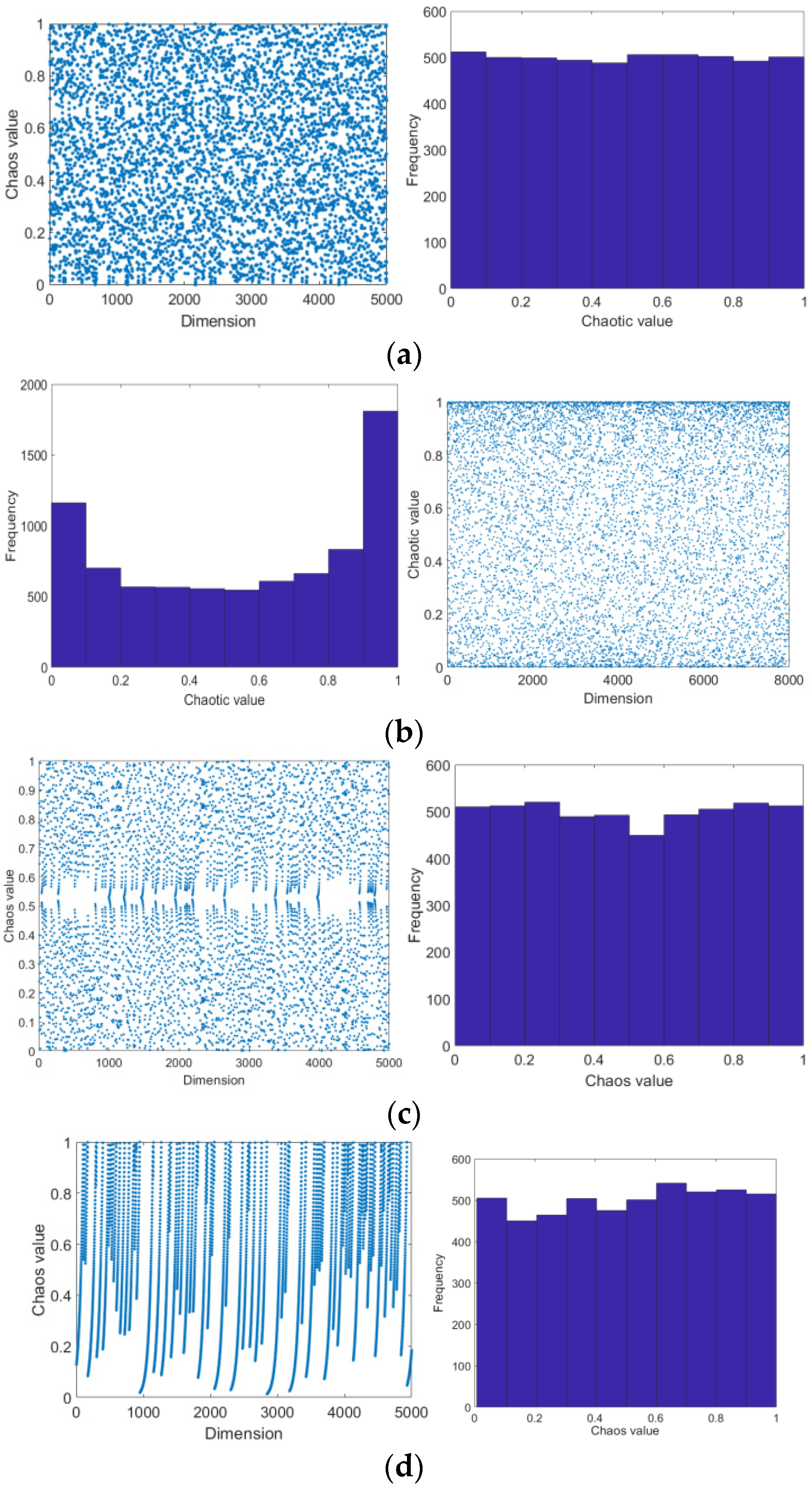
3.1. Tent Chaotic Map Initial Population

In the classical GWO algorithm, the initial population is usually randomly generated, which may lead to non-uniformity. The characteristics of the initial population affect the quality of the optimisation results of subsequent algorithms. However, chaotic motion has the opposite effect. It has the characteristics of high ergodicity, enabling the initial population to have high diversity; the advantages of chaotic motion can make the algorithm no longer limited to locally optimal solutions when solving function optimisation problems and strengthen the global search ability of the population. Existing chaotic maps include tent, logistic, and Henon maps. Different chaotic maps have different effects on the optimisation ability of the algorithm. Liang [23] proved that tent maps can produce more uniform ergodicity than other maps and further improve the optimisation speed of the algorithm. Therefore, in this study, the tent map was used to initialise the population.

Tent mapping has a simple structure and uniform distribution and is convenient. Its expression is as follows:

$$x_{n+1}=\left\{\begin{array}{c}\frac{x_n}{a},0\le x_n\le a\\ \frac{\left(1-x_n\right)}{1-a},a<x_n\le 1\end{array}\right.,$$

(7)

where $a\in \left(0,1\right)$. Repeated experiments have shown that the sequence generated during the period when $a=0.499$ was the most uniform. Therefore, the tent chaotic mapping formula quoted in this study can be expressed as

$$x_{n+1}=\left\{\begin{array}{c}\frac{x_n}{0.499},0\le x_n\le 0.499\\ \frac{\left(1-x_n\right)}{0.499},0.499<x_n\le 1\end{array}\right.,$$

(8)

here the coefficient $a=0.499$ is set, and tent mapping is iterated 5000 times. The distribution of values in the [0, 1] interval range is shown in Figure 2a. Compared with the logistic map in Figure 2b, the tent mapping distribution is more uniform and ergodic. The non-uniform initial population distribution under unset conditions can limit the algorithm’s search capabilities. In other words, the diversity of population distribution needs to be set manually. For instance, when a highly uniform initial population is required, the population should not be densely concentrated in local areas, which the logistic distribution fails to achieve.

Compared to pseudo-random data generation, tent chaotic mapping offers a more flexible setup for initial population parameters. Catering to the diverse requirements for initial population diversity does not necessarily imply that a more uniformly distributed population is always preferable. The optimal initial population varies based on the specific object being optimised. Although generating initial populations using pseudo-random numbers can achieve uniform distribution, it lacks diversity. The initialization of the initial population using the tent chaotic mapping is built upon random numbers. By adjusting the value of $a$, the distribution of the diverse population varies. As depicted in Figure 2c, setting $a=0.109$ results in a distinct ‘columnar’ correlated distribution within the population. However, when $a=0.98$, as depicted in Figure 2d, the distribution of the population within a certain range becomes extremely sparse, while other areas maintain a uniform distribution. Despite the differences in the initial population distributions, the frequency distribution of this initial population remains uniform.

3.2. Nonlinear Control Parameter Strategy

Generally, when searching for the global minimum, the optimisation algorithm can be divided into two basic stages. First, in the early stage of optimisation, individuals should be able to search the entire space to the extent possible to find more local minimum values. Second, in the later stage of optimisation, individuals should be encouraged to use the information they have collected to quickly converge to the global minimum. In the GWO algorithm, the value of $a$ affects the search methods of individuals. A larger control parameter $a$ is conducive to global exploration, while a smaller control parameter $a$ is conducive to local development. The parameter $a$ is adjusted to balance global exploration ability and local development ability.

However, in the traditional GWO algorithm, the value of the control parameter $a$ is linearly decreased from 2 to 0. Because the search process undertaken by the optimisation algorithm when solving practical problems should be nonlinear and highly complex, the strategy of linearly decreasing the parameter $a$ in the traditional GWO algorithm cannot accurately reflect the actual search process. Based on the above considerations, the equation for the control parameter $a$ was modified as follows:

$$\stackrel{\rightharpoonup }{a}\left(t\right)=a_{final}+\left(a_{final}-a_{initial}\right)\times {\left(\frac{Max\_iter-t}{Max\_iter}\right)}^{\mu },$$

(9)

where $t$ represents the current number of iterations, Max_iter is the total number of iterations, $\mu$ is the nonlinear modulation index, $a_{initial}$ and $a_{final}$ represents the initial and final values of the control parameter $a$, respectively.

Figure 3 shows the values of the control parameter $a$ under different values. Several experiments were conducted to test the role of the nonlinear modulation index $\mu$. The results show that when the nonlinear modulation index is $\mu =0.1$, the GWO algorithm exhibits better performance.

3.3. CSO Algorithm Coupling for an Improved GWO Algorithm

It is well known that in swarm intelligent optimisation algorithms such as particle swarm optimisation (PSO), ant colony optimisation (ACO), and artificial bee colony (ABC) optimisation, the balance between exploration and development capabilities has always been the object of research. It can be seen from the position update in Equations (5) and (6) in the traditional GWO algorithm that the path of grey wolves to hunt their prey is determined by the three optimal solutions, which means that $\omega$ individuals may not have sufficiently explored the global value. In other words, the traditional GWO is more likely to fall into the local optimal solution.

The core of the CSO_IGWO algorithm lies in the incorporation of the Lévy flight strategy. Inspired by the utilisation of the Lévy flight strategy in the CSO algorithm, this study leverages the characteristics of variable step size random walks in Lévy flights to enhance the position updating equation of the GWO algorithm. The introduction of the Lévy flight strategy enables individual grey wolves to undertake large leaps within their local positions and probabilistically expand the search region. This critical step ensures the GWO algorithm’s ability to break free from local optima. The Lévy distribution can be expressed using a simple power-law equation [24,25,26]:

$$L\left(s,\gamma ,\varpi \right)=\left\{\begin{array}{cc}\sqrt{\frac{\gamma }{2\pi }}\exp \left[-\frac{\gamma }{2\left(s-\varpi \right)}\right]\frac{1}{{\left(s-\varpi \right)}^{\frac{3}{2}}}\hfill & if0<\varpi <\infty \\ 0\hfill & otherwise\end{array}\right.,$$

(10)

where $s$ is the step size, $\varpi$ is the position or shift parameter, $\gamma >0$ is the scale parameter, and $L\left(s\right)$ represents the distribution of $s$.

The Lévy distribution can be expressed by a clear power law equation as:

$$L\left(s\right)~{\left|s\right|}^{-1-\beta }0<\beta \le 2.$$

(11)

The Mantegna strategy is also commonly used for simulations, and a normal distribution is used to solve the random step size. The method is as follows.

$$s=\frac{u}{{\left|v\right|}^{\frac{1}{\beta }}},$$

(12)

where $u$ and $v$ obey normal distribution.

To illustrate that the Lévy flight can achieve a high-frequency short step size and intermittent long step size, Figure 4 shows the motion tracks of the Lévy flight 50, 100, and 1000 times in two-dimensional space. The characteristics of the Lévy flight heavy-tail distribution can compensate for the disadvantage of the grey wolf algorithm, wherein it easily falls into a local optimal solution; it can also improve the ability of global optimisation.

Therefore, in combination with the Lévy flight concept in the CSO algorithm, a new position update formula is obtained as follows:

$$\Delta \stackrel{\rightharpoonup }{X}\left(t+1\right)=\left\{\begin{array}{c}\stackrel{\rightharpoonup }{X}\left(t+1\right)\\ \stackrel{\rightharpoonup }{X}\left(t+1\right)+\epsilon \oplus Levy\left(\beta \right)\end{array}\begin{array}{c}\left|A\right|<1\\ \left|A\right|>1\end{array}\right.,$$

(13)

where $\epsilon =0.01\cdot \left(X^t-X_{best}^t\right)$ is the step control parameter, $X^t$ and $X_{best}$ represent the t-generation individual and the t-generation optimal individual, respectively. When $\left|A\right|>1$, the grey wolf is far away from the prey, and when $\left|A\right|<1$, the grey wolf is close to the prey. This study combines the Lévy flight strategy in the CSO algorithm with an improved GWO algorithm to develop the CS_GWO algorithm. The CS is given in Algorithm 1, along with the pseudocode for GWO.

Algorithm 1 CSO_GWO algorithm.

Initialising population with a chaotic tent map Initialise $A$, $C$, and $\alpha$ Calculate the fitness value of each individual $X_{\alpha }$ = Best individual $X_{\beta }$ = Suboptimal individual $X_{\delta }$ = Third best individual While (t < Max_iter)    For each individual in the population       Use Equation (13) to update the current position of the individual    End for    Update $\alpha$ with Equation (9)    Update A and C with Equation (3) Calculate fitness of all individuals Update $X_{\alpha }$, $X_{\beta }$ and $X_{\delta }$ $t=t+1$ End While Return $X_{\alpha }$

The research on the proposed optimisation algorithm is conducted in three main aspects. Firstly, the distribution of the population: the tent mapping initialization of the population imparts richer distribution characteristics to the initial population. It enables both uniform distribution across the entire region and sparse distribution in local areas. Secondly, the introduction of a nonlinear control strategy governs the process of searching for the optimal values within the population. It ensures that the population conducts broad-scale searches in the initial phase, followed by localised refinement to find the optimal solution. Lastly, the integration of the Lévy flight strategy from the CSO algorithm empowers the first two aspects with the characteristic of significant leaps in Lévy flights. This infusion of large-scale jumping abilities from Lévy flights allows the algorithm proposed in this paper to achieve both a broad search scope and the ability to find optimal values within local regions.

4. Numerical Data Experiment and Simulation Analysis

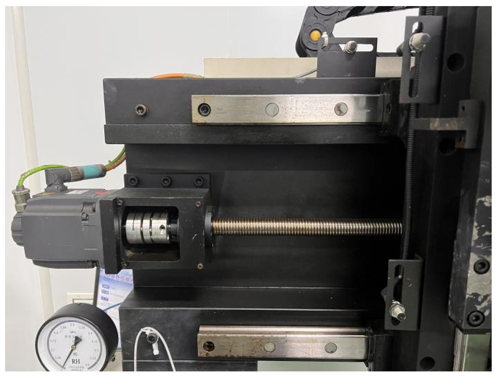
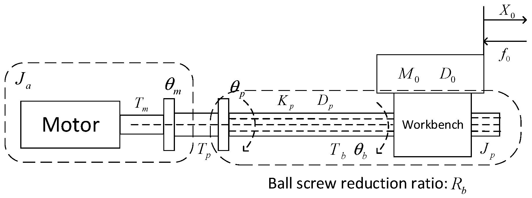
4.1. Mathematical Model of a Servo Motor System

In recent years, with the increasing industrialization levels in China, servo control systems have been widely used in all walks of life, from industrial production of mechanical arms to computer numerical control (CNC) machine tools, military weapon servo systems, and even aerospace satellites. Servo control systems are ubiquitous in use. The motor control determines the working performance of the entire system as the main component of the servo system. Therefore, it is necessary to study the drive control part of the servo motor in depth [27,28].

The experiment in this section is conducted on a self-developed small CNC polishing machine. This equipment has three linear axes (X, Y, and Z) and two rotational axes (A and C). To validate the practicality of the optimisation algorithm proposed in this paper, an experimental motion control of the Y-axis, whose model is Somotics s-1fk7(SIEMENS, Munich, Germany), was performed on this machine. The physical illustration is depicted in Figure 5.

The servomotor model is shown in Figure 6; it includes the motor, coupling, roller lead screw, guide rail, and workbench. Driven by the motor, the ball screw and motor are coaxially rotated through the coupling, so that the rotating motion of the rotating motor is transformed into the linear motion of the workbench. The symbols in the figure are listed in

Table 1. Symbols used for the servo motor model.

Symbol	Physical Meaning	Parameter
$J_a$	Moment of inertia of the drive shaft	$0.1 \mathrm{kg}\cdot {\mathrm{m}}^2$
$T_m$	Motor output torque	$50 \mathrm{N}\cdot \mathrm{m}$
$K_p$	Torsional stiffness coefficient of a driven shaft	$899 \mathrm{Nm}/\mathrm{rad}$
$T_b$	Output torque of a ball screw driven by a driven shaft	$50 \mathrm{N}\cdot \mathrm{m}$
$M_0$	Moving platform mass	$38 \mathrm{kg}$
$X_0$	Moving platform displacement	0–130 cm
$T_p$	Coupling transmission output torque	$50 \mathrm{N}\cdot \mathrm{m}$
$J_p$	Moment of inertia of a driven shaft	0.15 kg·m2
${\theta }_m$	Motor output angle	0–360°
$D_p$	Driven shaft damping coefficient	$3.83 \mathrm{Nm}/\mathrm{rad}$
${\theta }_b$	Output angle of a ball screw driven by a driven shaft	0–360°
$D_0$	Damping coefficient of a moving platform	$10 \mathrm{Ns}/\mathrm{m}$
$f_0$	Load resistance of a moving platform	$44 \mathrm{N}\cdot \mathrm{m}$
${\theta }_p$	Coupling transmission output angle	0–360°

.

According to the servo motor model shown in Figure 5, the dynamic differential equation can be obtained as follows:

$$T_b=\frac{J_0{\ddot{\theta }}_b+D_0{\dot{\theta }}_b+f_0{R}_b}{R_b^2},$$

(14)

$$T_m=J_a{\ddot{\theta }}_m+T_p,$$

(15)

$$T_p=K_p\left({\theta }_p-{\theta }_b\right)+D_p\left({\dot{\theta }}_p-{\dot{\theta }}_b\right)=J_p{\ddot{\theta }}_b+T_b.$$

(16)

The above dynamic differential equation is further simplified into a transfer function form by the Laplace transformation:

$${\theta }_b\left(s\right)\approx \frac{R_b^2\left(k_p+D_{p}s\right){\theta }_p\left(s\right)}{\left(J_p{R}_b^2+M_0\right)s^2+\left(D_0+R_b^2{D}_p\right)s+R_b^2{k}_p}.$$

(17)

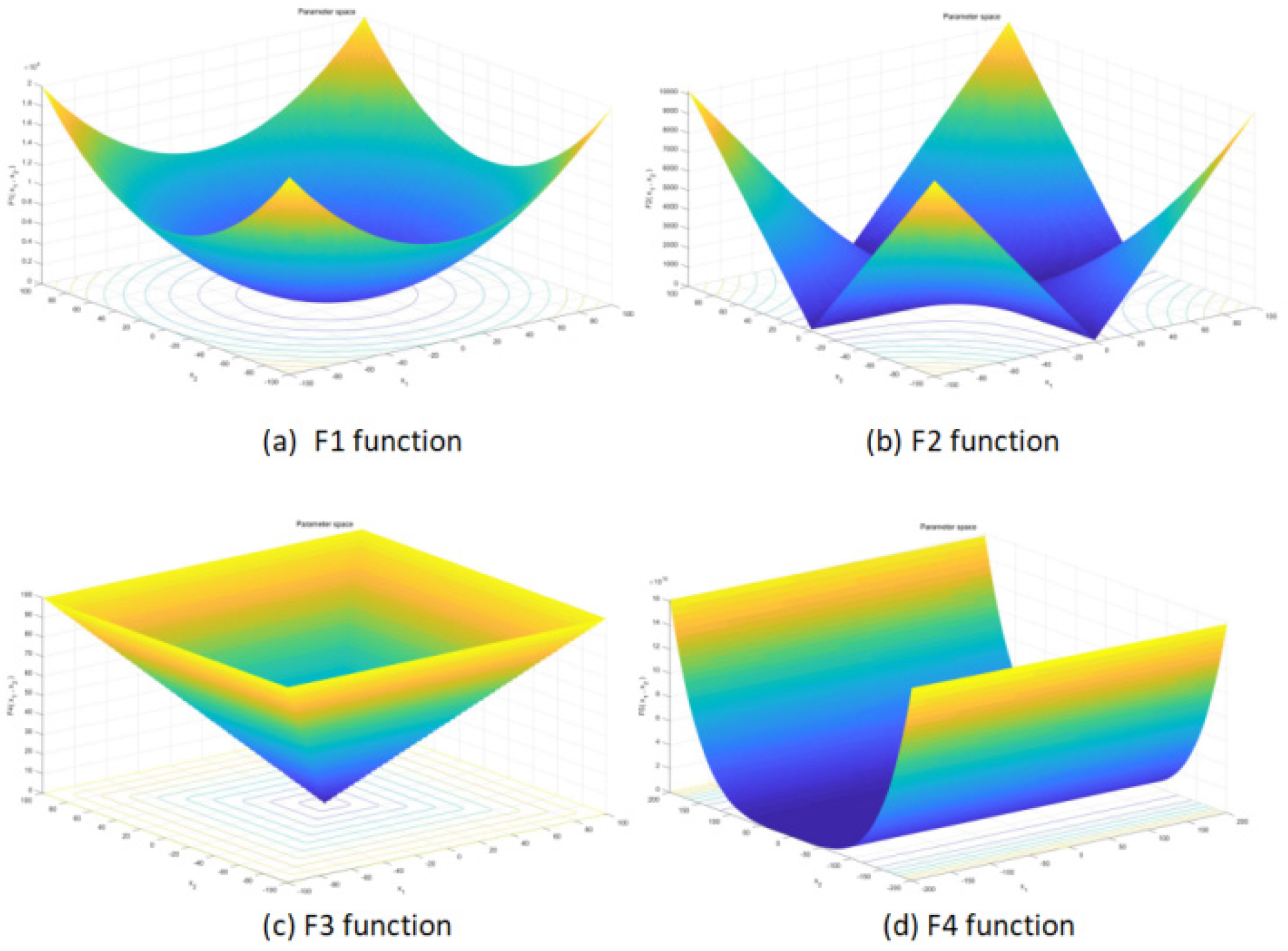
4.2. Benchmark Functions

To test the effectiveness of the improved GWO algorithm in this study, eight of the widely used “23” benchmark functions [29] were selected to test the improved algorithm and compare the traditional GWO with the improved GWO. The benchmark functions can be divided into two categories: unimodal (F1–F4), as shown in Figure 7, and multimodal (F5–F8), as shown in Figure 8. The unimodal functions are suitable for testing the exploration ability of the algorithm because they have a global optimum and no local optimum, whereas multimodal functions have considerable local optimality, which is helpful for testing the development ability of the algorithms. See

Table 2. Benchmark functions.

Function	Dim	Range	${\mathit{f}}_{\mathbf{min}}$
$F_1\left(x\right)={\displaystyle \sum _{i=1}^{30}{x}_i^2}$	30	[−100, 100]	0
$F_2\left(x\right)={\displaystyle \sum _{i=1}^{30}\left|x_i\right|}+{\displaystyle \coprod _{i=1}^{30}\left|x_i\right|}$	30	[−10, 10]	0
$F_3\left(x\right)={\max }_i\left\{\left|x_i\right|,1\le i\le 30\right\}$	30	[−100, 100]	0
$F_4\left(x\right)={\displaystyle \sum _{i=1}^{30}\left[100{\left(x_{i+1}-x_i^2\right)}^2+{\left(x_i-1\right)}^2\right]}$	30	[−30, 30]	0
$F_5\left(x\right)={\displaystyle \sum _{i=1}^{30}i{x}_i^4+random[0,1)}$	30	[−1.28, 1.28]	0
$F_6\left(x\right)={\displaystyle \sum _{i=1}^{30}{x}_i^2-10\cos \left(2\pi x_i\right)+10}$	30	[−5.12, 5.12]	0
$\begin{array}{l}{F}_7\left(x\right)=-20\exp \left(-0.2\sqrt{\frac{1}{n}{\displaystyle \sum _{i=1}^{30}{x}_i^2}}\right)-\\ \begin{array}{ccc}& & \exp \left(\frac{1}{n}{\displaystyle \sum _{i=1}^{30}\cos \left(2\pi x_i\right)}\right)\end{array}+20+e\end{array}$	30	[−5.12, 5.12]	0
$\begin{array}{l}{F}_8\left(x\right)=0.1\left\{\begin{array}{l}{\sin }^2\left(3\pi x_1\right)+\\ {\displaystyle \sum _{i=1}^{30}\begin{array}{l}{\left(x_i-1\right)}^2\left[1+{\sin }^2\left(3\pi x_i+1\right)\right]+\\ {\left(x_n-1\right)}^2\left[1+{\sin }^2\left(2\pi x_n\right)\right]\end{array}}\end{array}\right\}\\ \begin{array}{ccc}& & +{\displaystyle \sum _{i=1}^{n}u\left(x_i,5,100,4\right)}\end{array}\end{array}$	30	[−50, 50]	0

for the specific benchmark functions.

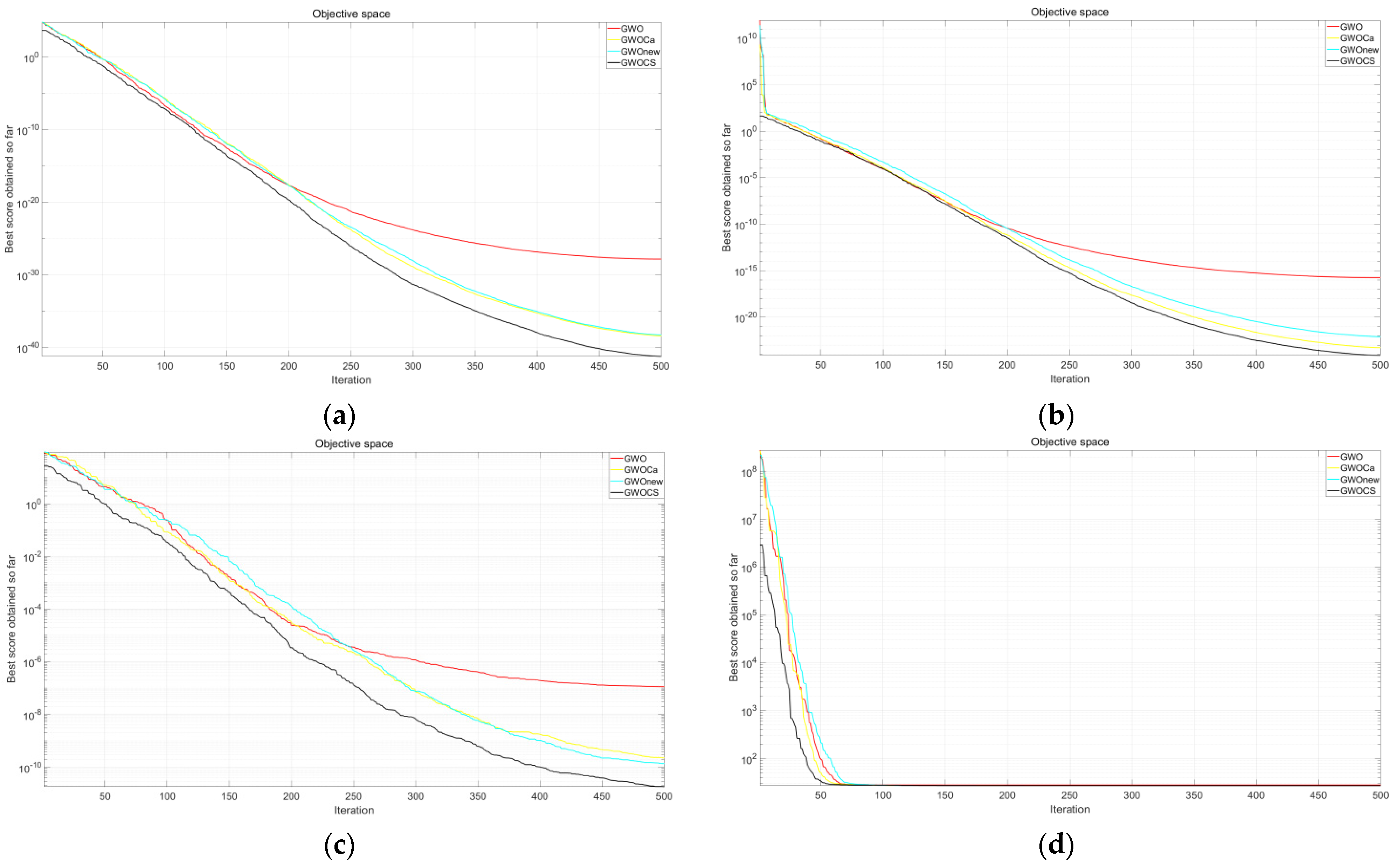
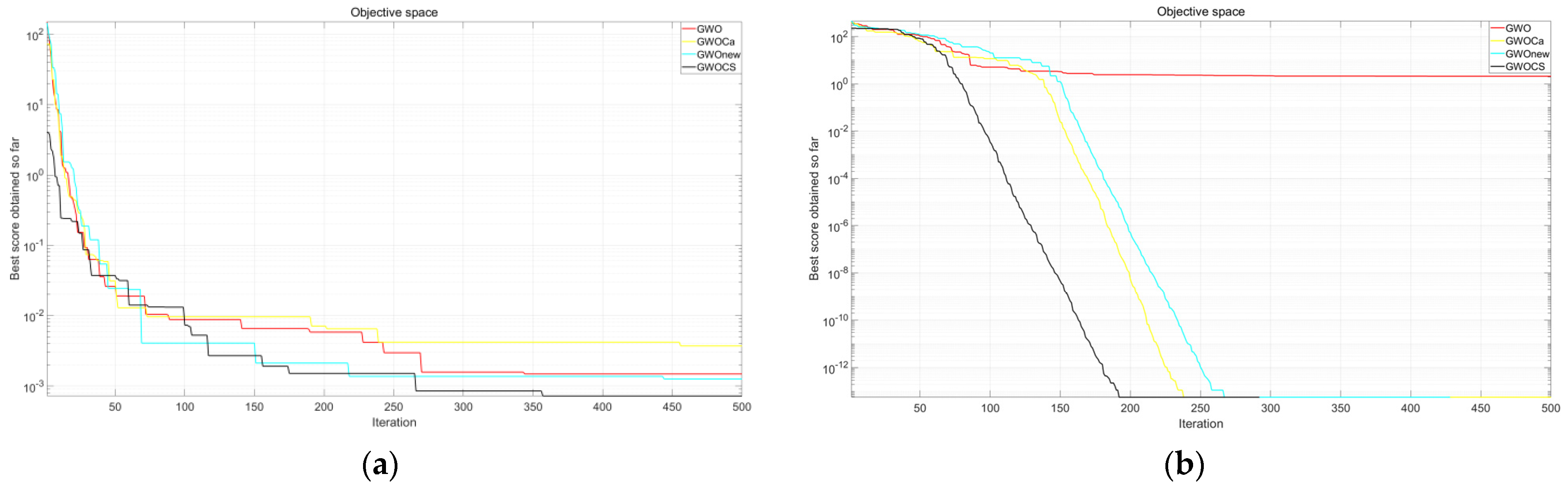
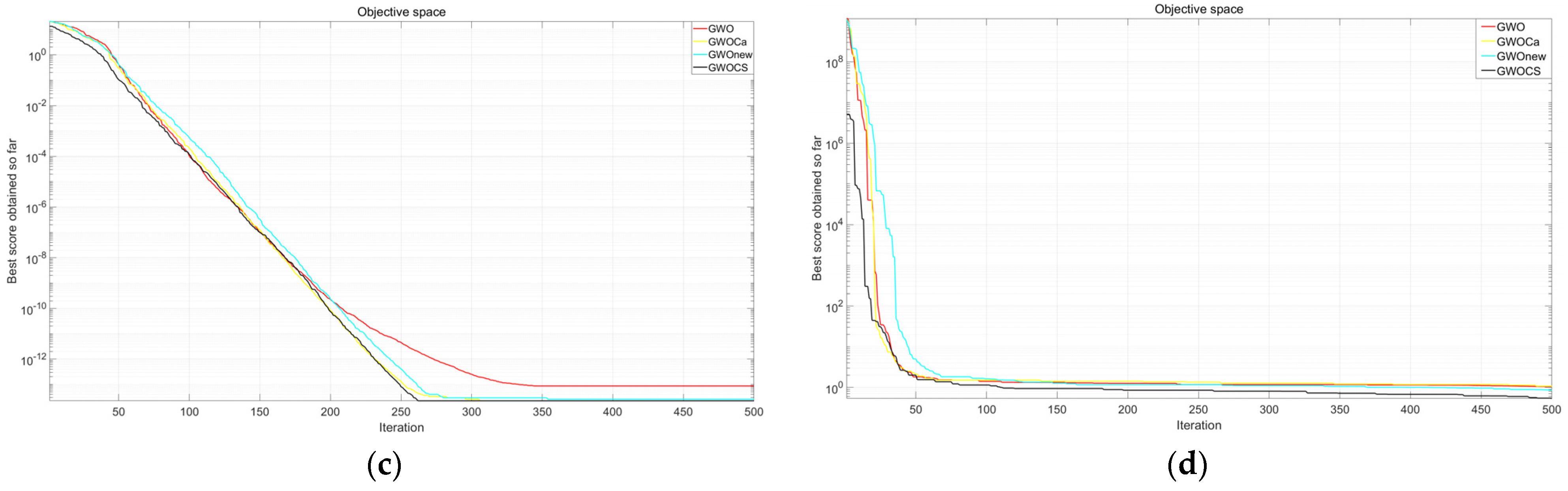
4.3. Comparison with the Traditional GWO Algorithm

To verify the superiority of the CSO_IGWO algorithm, the GWO and CSO_IGWO algorithms were set with the same common control parameters. In all function optimisations, the population size (N) was 30, and the maximum number of iterations (Max_iter) was 500. Other specific parameters of the CGO algorithm were set as follows: nonlinear modulation index $\mu =1.5$, $a_{initial}=0$, and $a_{final}=2$. The CSO_IGWO and traditional GWO algorithms were coded in MATLAB 2017b. All experiments were conducted on a computer using an Intel (R) Core (TM) i5-8265U [email protected] GHz and 8.00 GB of RAM (Intel, Shanghai, China).

In this section, to verify the superiority of the proposed CSO_IGWO algorithm, the eight benchmark test functions shown in Table 2 were tested. Independent experiments were used to compare the CSO_IGWO algorithm with the traditional GWO algorithm, the GWO_a algorithm that changes the control parameter $a$, and the GWO_NEW algorithm, which improves the initial population. To reduce the chance of testing, each function was tested 30 times, and the average value and standard deviation of the functions were obtained. The optimal results are highlighted in bold. The experimental results are listed in

Table 3. Experimental results.

Function	Dim	Mean	STD	Mean	STD
		GWO		GWO_a
F1	30	8.2498 × 10−28	9.20958 × 10−28	2.69527 × 10−39	3.35115 × 10−39
F2	30	1.03689 × 10−16	6.84302 × 10−17	1.28624 × 10−23	9.90575 × 10−24
F3	30	9.80503 × 10−7	7.64443 × 10−7	3.10067 × 10−10	2.6378 × 10−10
F4	30	27.26432	0.730128317	2.68 × 10	0.577598699
F5	30	2.06 × 10−3	0.000839552	1.603 × 103	7.747 × 104
F6	30	7.38971 × 10−14	2.60506 × 10−14	0	0
F7	30	1.07 × 10−13	1.473 × 10−14	2.007 × 10−15	4.263 × 10−16
F8	30	6.70 × 10−1	1.979 × 10−1	5.495 × 10−1	1.307 × 10−1
		GWO_NEW		CSO_IGWO
F1	30	5.07317 × 10−39	5.45724 × 10−39	5.48004 × 10−40	5.22096 × 10−40
F2	30	6.76155 × 10−24	4.77805 × 10−24	6.434 × 10−24	3.31312 × 10−24
F3	30	3.63217 × 10−10	2.96633 × 10−10	8.10248 × 10−11	7.43226 × 10−11
F4	30	27.12109	0.549138876	2.66 × 10	0.59195957
F5	30	1.658 × 103	8.374 × 104	5.81 × 10−4	2.323 × 104
F6	30	0	0	0	0
F7	30	2.114 × 10−15	5.037 × 10−16	1.54 × 10−16	2.505 × 10−17
F8	30	7.423 × 10−1	1.451 × 10−1	3.82 × 10−1	1.299 × 10−1

.

To further illustrate the advantages of CSO_IGWO over IGWO and GWO in some typical problems, their unimodal and multimodal convergence curves are shown in Figure 9 and Figure 10. It can be observed from the figure that for the above eight benchmark functions, the CSO_IGWO algorithm is faster than the classical GWO algorithm and can jump out of the local optimum. This shows that using the cuckoo algorithm to improve the grey wolf algorithm not only improves the search accuracy but also optimises the global search speed.

4.4. Analysis of the Parameter Setting Experiment

When adopting a swarm intelligence optimisation algorithm to adjust the controller parameters, the frequently selected objective functions are generally divided into two types: integral square error (ISE) and (Integrated Time and Absolute Error) ITAE. The selection of different objective functions directly affects controller performance [30]. In engineering applications, most controlled systems are nonlinear, and the above three objective functions do not consider whether the output u(t) exceeds the physical limit, which leads to controller design failure. Therefore, the integral absolute error (IAE) was used to minimise the objective function, and the maximum output value of the controller was used as a penalty function to optimise the controller design and parameter tuning. Therefore, the objective function is written as:

$$f\left(t\right)={\displaystyle {\int }_0^{\infty }\left({\omega }_1\left|e\left(t\right)\right|+{\omega }_2{u}^2\left(t\right)\right)dt+{\omega }_3{t}_u},$$

(18)

where $e\left(t\right)$ is the system error; $u\left(t\right)$ is the controller output; $t_u$ is the rise time; and ${\omega }_1$,${\omega }_2$, and ${\omega }_3$ are the weights.

The iterative steps of the controller algorithm are as follows:

• Step 1: Initialise the parameters of CWO, such as population size N, maximum iterations (Max_iter), initial value ${\stackrel{\rightharpoonup }{a}}_{initial}$, final value ${\stackrel{\rightharpoonup }{a}}_{final}$ of $\stackrel{\rightharpoonup }{a}$, parameters A and C, and the nonlinear modulation index $\mu$;
• Step 2: Use tent mapping to generate individual populations $\left\{X_i,i=1,2,3\dots ,N\right\}$ and calculate the fitness value $\left\{f_i,i=1,2,3\dots ,N\right\}$ of each individual;
• Step 3: The fitness function value for each candidate is calculated. According to the order of fitness values from large to small, the individuals corresponding to the first three fitness values are taken as $\alpha$, $\beta$, and $\delta$, and their corresponding location information is respectively $X_{\alpha }$, $X_{\beta }$, and $X_{\delta }$;
• Step 4: To find the best location of prey, use Equation (9) to calculate the nonlinear change parameter $\stackrel{\rightharpoonup }{a}$, and then update the A and C values according to Equation (3);
• Step 5: Use Equation (13) to update the position of population individuals, recalculate fitness values, and update the $\alpha$, $\beta$, and $\delta$ values;
• Step 6: Determine whether $t$ reaches the Max_iter value; if it is reached, the best solution (that is, the fitness value of $X_{\alpha }$) will be output; otherwise, return to Step 3 to continue execution.

The motor model proposed in Section 4.1 is used as the controlled object of the traditional GWO algorithm and the CSO_IGWO algorithm experiment, and the function value convergence curve of the objective function is shown in Figure 11. It can be seen from the iteration curve that the CWO algorithm improved the optimisation upper limit, making the parameter optimisation more accurate, unlike the traditional GWO algorithm, which has fallen into the local optimal solution early. This is because of the idea of using the Lévy flight strategy in the CSO_IGWO algorithm to improve the GWO algorithm and taking advantage of the Lévy flight strategy to make the GWO algorithm jump out of the local optimisation.

To verify the superiority of the algorithm proposed in this paper and further compare its convergence with other swarm intelligence optimisation algorithms, two more classical and widely used swarm intelligence optimisation algorithms were selected: an improved particle swarm optimisation algorithm and an improved genetic algorithm. The iteration comparison curve is shown in Figure 12. It can be seen from the figure that the algorithm proposed in this paper is not only considerably better than the other three optimisation algorithms in terms of search breadth but also has the ability to jump out of the local optimum.

The open-loop response of the motor model is shown in Figure 13 It can be observed that the dynamic response performance under the open-loop is not ideal; the overshoot is too large, and the adjustment time is too long.

Figure 14 shows the four parameter-tuning methods and open-loop Bode diagram of the system. It can be seen from the figure that for the servomotor model selected in this study, the phase margin under the four controllers is positive, and the phase near the cut-off frequency (10 rad/s) is smooth, indicating that the system is robust when the control gain fluctuates within a certain range.

To reflect the superiority of the CSO_IGWO algorithm in tuning PID control parameters, the parameter tuning method proposed in this paper is compared with the traditional Z–N method, the improved particle swarm optimisation algorithm, and the improved genetic optimisation algorithm, as shown in Figure 15.

The performance indicators are presented in

Table 4. Comparison of experimental results.

Tuning Method	${\mathit{T}}_{\mathit{r}}/\mathbf{s}$	$\mathit{M}\mathit{p}/\mathit{\%}$	${\mathit{T}}_{\mathit{s}}/\mathbf{s}$	${\mathit{E}}_{\mathit{s}\mathit{s}}/\mathit{\%}$
None	1.75	52.451	30.67	2
Z–N method	2.0724	25.374	8.289	0
IPSO method	1.381	14.1	7.726	0
IGA method	4.483	4.6	7.291	0
CSO_IGWO method	2.1316	4.5911	4.021	0

. It can be seen from the table that the traditional Ziegler–Nichols (Z–N) method for tuning the PID controller parameters can improve the dynamic performance of the controlled system, but compared with the CSO_IGWO algorithm for optimising PID control parameters, the CSO_IGWO algorithm for optimising dynamic performance is more obvious. However, the improved particle swarm optimisation (IPSO) algorithm and the improved genetic optimisation (IGA) algorithm clearly show their defects and easily fall into local optima. These fall into different local optimum solutions. The PID parameter overshoot under the improved genetic algorithm is large, whereas the PID parameter overshoot under the improved particle swarm optimisation algorithm is small but very slow. Through comparison, the parameter tuning method proposed in this study can help the system achieve satisfactory performance.

5. Conclusions

The cuckoo search optimisation coupled with the improved grey wolf optimisation algorithm for tuning the PID parameters proposed in this study is improved in three aspects: initial population, control parameters, and position equations. The improved algorithm can effectively avoid premature convergence, accelerate the iteration time, and improve parameter accuracy. Two simulation experiments are conducted. First, eight benchmark functions were used to verify the superiority of the improved algorithm. The experimental results show that the overall iteration speed is accelerated, and it is not easy to fall into the local optimal solution for multimodal benchmark function problems.

By comparing the PID parameter tuning method proposed in this paper with other parameter tuning methods, it can be concluded that the proposed CSO_GWO method significantly enhances the dynamic performance of motors under PID control. The method’s efficiency in tuning PID parameters allows swift computations, facilitating its application in practical motion control scenarios. Even in the presence of external influences, this approach substantially improves motor control performance, preventing the parameter tuning process from converging to a suboptimal region due to external disturbances. Fine-tuning the three key parameters of the PID algorithm achieves optimal motor dynamic performance.

However, certain limitations persist. The computational complexity of this algorithm and its extensive calculation procedures render it unsuitable for real-time online adjustment of controller parameters. Moreover, when applied to more complex advanced control algorithms, the cumulative computational load of tuning parameters and the intricate advanced control algorithm significantly increase the overall process time. Consequently, future research needs to focus on further optimising the algorithmic procedures and evolving the proposed method to be compatible with a broader array of advanced algorithms.

References

1. O’Dwyer, A. PI and PID Controller Tuning Rules for Time Delay Processes: A Summary. In Proceedings of the Irish Signals and Systems Conference, Dublin, Ireland, June 1999; Available online: https://arrow.tudublin.ie/cgi/viewcontent.cgi?article=1074&context=engscheleart (accessed on 1 November 2023).
2. Joseph, S.B.; Dada, E.G.; Abidemi, A.; Oyewola, D.O.; Khammas, B.M. Metaheuristic algorithms for PID controller parameters tuning: Review, approaches and open problems. Heliyon 2022, 8, e09399. [Google Scholar] [CrossRef] [PubMed]
3. Nabati, E.G.; Engell, S. Online Adaptive Robust Tuning of PID Parameters. IFAC Proc. Vol. 2012, 45, 625–630. [Google Scholar] [CrossRef]
4. Borase, R.P.; Maghade, D.K.; Sondkar, S.Y.; Pawar, S.N. A review of PID control, tuning methods and applications. Int. J. Dyn. Control. 2021, 9, 818–827. [Google Scholar] [CrossRef]
5. Guo, Y.-Q.; Zha, X.-M.; Shen, Y.-Y.; Wang, Y.-N.; Chen, G. Research on PID position control of a hydraulic servo system based on kalman genetic optimization. Actuators 2022, 11, 162. [Google Scholar] [CrossRef]
6. Xiao, L. Parameter tuning of PID controller for beer filling machine liquid level control based on improved genetic algorithm. Comput. Intell. Neurosci. 2021, 2021, 7287796. [Google Scholar] [CrossRef] [PubMed]
7. Cárdenas, J.A.; Carrero, U.E.; Camacho, E.C.; Calderón, J.M. Optimal PID ø axis Control for UAV Quadrotor based on Multi-Objective PSO. IFAC-PapersOnLine 2022, 55, 101–106. [Google Scholar] [CrossRef]
8. Ye, Y.; Yin, C.-B.; Gong, Y.; Zhou, J.-J. Position control of nonlinear hydraulic system using an improved PSO based PID controller. Mech. Syst. Signal Proc. 2017, 83, 241–259. [Google Scholar] [CrossRef]
9. Mirjalili, S.; Mirjalili, S.M.; Lewis, A. Grey wolf optimizer. Adv. Eng. Softw. 2014, 69, 46–61. [Google Scholar] [CrossRef]
10. Fei, G. Overview of the Application of Genetic Algorithms in the Field of Automatic Control. Electron. World 2017, 9, 51. [Google Scholar] [CrossRef]
11. Xiang, Z.; Ji, D.; Zhang, H.; Wu, H.; Li, Y. A simple PID-based strategy for particle swarm optimization algorithm. Inf. Sci. 2019, 502, 558–574. [Google Scholar] [CrossRef]
12. Rodríguez, L.; Castillo, O.; Soria, J.; Melin, P.; Valdez, F.; Gonzalez, C.I.; Martinez, G.E.; Soto, J. A fuzzy hierarchical operator in the grey wolf optimizer algorithm. Appl. Soft Comput. 2017, 57, 315–328. [Google Scholar] [CrossRef]
13. Kumar, V.; Kumar, D. An astrophysics-inspired Grey wolf algorithm for numerical optimization and its application to engineering design problems. Adv. Eng. Softw. 2017, 112, 231–254. [Google Scholar] [CrossRef]
14. Heidari, A.A.; Pahlavani, P. An efficient modified grey wolf optimizer with Lévy flight for optimization tasks. Appl. Soft Comput. 2017, 60, 115–134. [Google Scholar] [CrossRef]
15. Chinglemba, T.; Biswas, S.; Malakar, D.; Meena, V.; Sarkar, D.; Biswas, A. Introductory Review of Swarm Intelligence Techniques. In Advances in Swarm Intelligence: Variations and Adaptations for Optimization Problems; Springer: Berlin/Heidelberg, Germany, 2022; pp. 15–35. [Google Scholar]
16. Selvaraj, S.; Choi, E. Survey of swarm intelligence algorithms. In Proceedings of the 3rd International Conference on Software Engineering and Information Management, Sydney, Australia, 12–15 January 2020; pp. 69–73. [Google Scholar]
17. Phan, H.D.; Ellis, K.; Barca, J.C.; Dorin, A. A survey of dynamic parameter setting methods for nature-inspired swarm intelligence algorithms. Neural Comput. Appl. 2020, 32, 567–588. [Google Scholar] [CrossRef]
18. Zhao, Z.Q.; Liu, S.J.; Pan, J.S. A PID parameter tuning method based on the improved QUATRE algorithm. Algorithms 2021, 14, 173. [Google Scholar] [CrossRef]
19. Soleimani Amiri, M.; Ramli, R.; Ibrahim, M.F.; Abd Wahab, D.; Aliman, N. Adaptive particle swarm optimization of PID gain tuning for lower-limb human exoskeleton in virtual environment. Mathematics 2020, 8, 2040. [Google Scholar] [CrossRef]
20. Caponetto, R.; Fortuna, L.; Porto, D. Parameter tuning of a non integer order PID controller. In Proceedings of the Fifteenth International Symposium on Mathematical Theory of Networks and Systems, Notre Dame, IN, USA, 12–16 August 2002. [Google Scholar]
21. Altintas, G.; Aydin, Y. Optimization of fractional and integer order PID parameters using big bang big crunch and genetic algorithms for a MAGLEV system. IFAC-PapersOnLine 2017, 50, 4881–4886. [Google Scholar] [CrossRef]
22. Yang, R.; Liu, Y.; Yu, Y.; He, X.; Li, H. Hybrid improved particle swarm optimization-cuckoo search optimized fuzzy PID controller for micro gas turbine. Energy Rep. 2021, 7, 5446–5454. [Google Scholar] [CrossRef]
23. Shan, L.; Qiang, H.; Li, J.; Wang, Z. Chaotic optimization algorithm based on Tent mapping. Control Decis. Mak. 2005, 20, 179. [Google Scholar] [CrossRef]
24. Wang, Z.; Chen, Y.; Ding, S.; Liang, D.; He, H. A novel particle swarm optimization algorithm with Lévy flight and orthogonal learning. Swarm Evol. Comput. 2022, 75, 101207. [Google Scholar] [CrossRef]
25. Guerrero-Luis, M.; Valdez, F.; Castillo, O. A Review on the Cuckoo Search Algorithm. In Fuzzy Logic Hybrid Extensions of Neural and Optimization Algorithms: Theory and Applications; Springer: Berlin/Heidelberg, Germany, 2021; pp. 113–124. [Google Scholar] [CrossRef]
26. Hussein, W.A.; Sahran, S.; Abdullah, S.N.H.S. Patch-Levy-based initialization algorithm for Bees Algorithm. Appl. Soft Comput. 2014, 23, 104–121. [Google Scholar] [CrossRef]
27. Kommuri, S.K.; Defoort, M.; Karimi, H.R.; Veluvolu, K.C. A Robust Observer-Based Sensor Fault-Tolerant Control for PMSM in Electric Vehicles. IEEE Trans. Ind. Electron. 2016, 63, 7671–7681. [Google Scholar] [CrossRef]
28. Li, S.; Liu, H.; Fu, W. An Improved Predictive Functional Control Method with Application to PMSM systems. Int. J. Electron. 2016, 104, 126–142. [Google Scholar] [CrossRef]
29. Long, W.; Cai, S.; Jiao, J.; Zhang, W.-Z.; Tang, M.-Z. A hybrid grey wolf optimization algorithm for high-dimensional optimization problems. Control Decis. 2016, 31, 1991. [Google Scholar] [CrossRef]
30. Gao, Z.-M.; Zhao, J. An improved grey wolf optimization algorithm with variable weights. Comput. Intell. Neurosci. 2019, 2019, 2981282. [Google Scholar] [CrossRef]
Figure 1. Hierarchy of the grey wolf group.
Applsci 13 12944 g001
Figure 2. (a) Tent mapping. (b) Logistic mapping. (c) Tent mapping, a = 0.109. (d) Tent mapping, a = 0.98.
Applsci 13 12944 g002
Figure 3. Change curve of control parameter a under different μ values.
Applsci 13 12944 g003
Figure 4. Trajectories of Lévy flying 50, 100, and 1000 times in two-dimensional space. (a) Trajectories of Lévy flying 50 times in two-dimensional space, (b) Trajectories of Lévy flying 100 times in two-dimensional space, and (c) Trajectories of Lévy flying 1000 times in two-dimensional space.
Applsci 13 12944 g004aApplsci 13 12944 g004b
Figure 5. The physical illustration of the Y-axis.
Applsci 13 12944 g005
Figure 6. Servo motor model.
Applsci 13 12944 g006
Figure 7. Unimodal benchmark functions.
Applsci 13 12944 g007
Figure 8. Multimodal benchmark functions.
Applsci 13 12944 g008
Figure 9. (ad) Convergence curves of unimodal benchmark functions. (a) F1 Function, (b) F2 Function, (c) F3 Function, and (d) F4 Function.
Applsci 13 12944 g009
Figure 10. (ad) Convergence curves of the multimodal benchmark functions. (a) F5 Function, (b) F6 Function, (c) F7 Function, and (d) F8 Function.
Applsci 13 12944 g010aApplsci 13 12944 g010b
Figure 11. GWO and CSO_IGWO iteration comparison curve.
Applsci 13 12944 g011
Figure 12. Iteration comparison curve of four optimisation algorithms.
Applsci 13 12944 g012
Figure 13. Open-loop step response curve of the system.
Applsci 13 12944 g013
Figure 14. Bode diagram of system response.
Applsci 13 12944 g014
Figure 15. Comparison curves of system step responses.
Applsci 13 12944 g015