

A Java Application for Teaching Graphs in Undergraduate Courses


Abstract
:1. Introduction
2. MaGraDa Software Tool
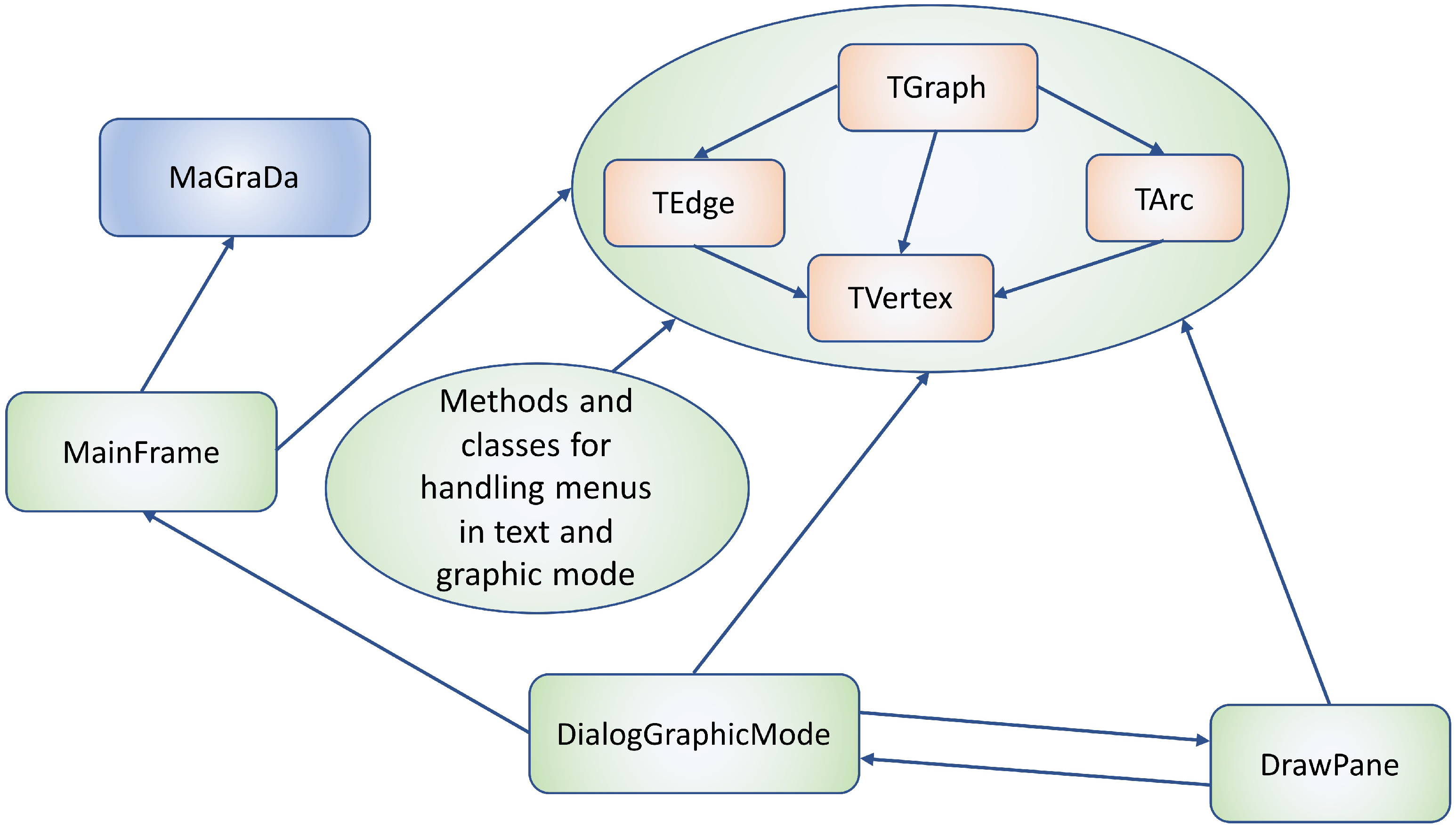
2.1. Structure and Design of the Software Tool
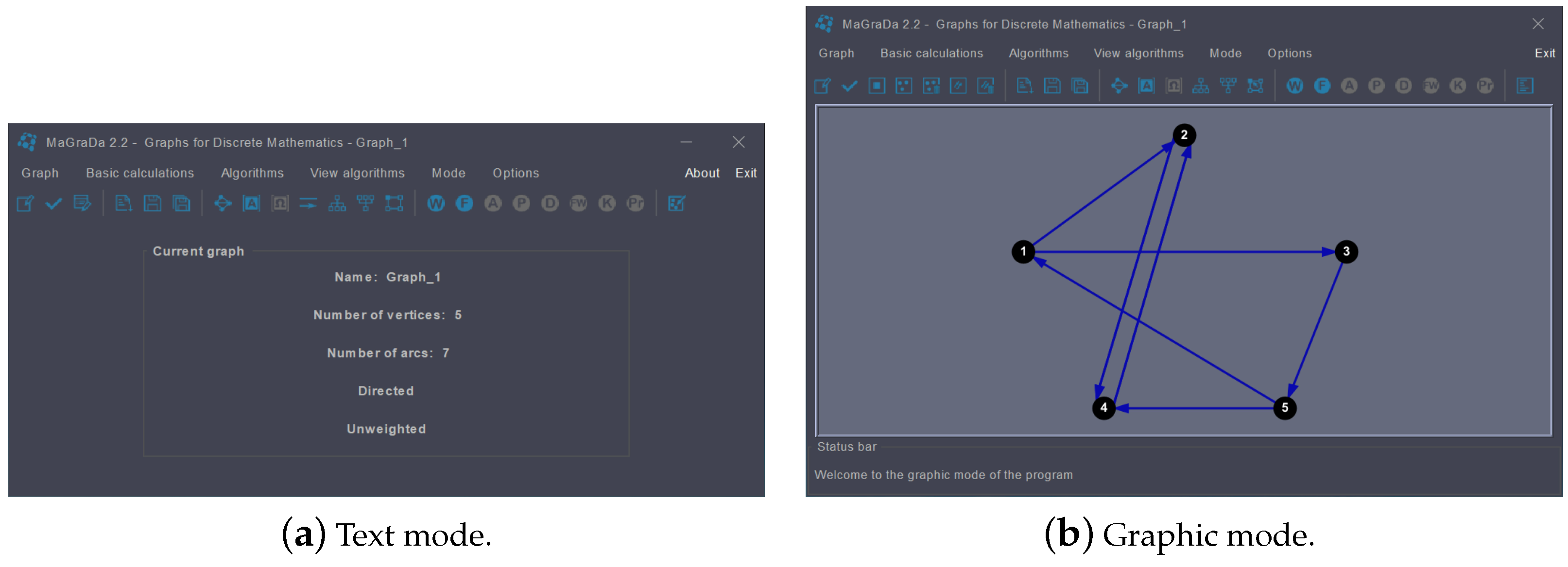
2.2. Description of the Visualisation and Computational Tool
- Graph menu: This allows for the handling of graphs.
- Basic calculations menu: This gives some basic properties of the current graph.
- Algorithms menu: This shows the algorithms that are available to apply to the current graph.
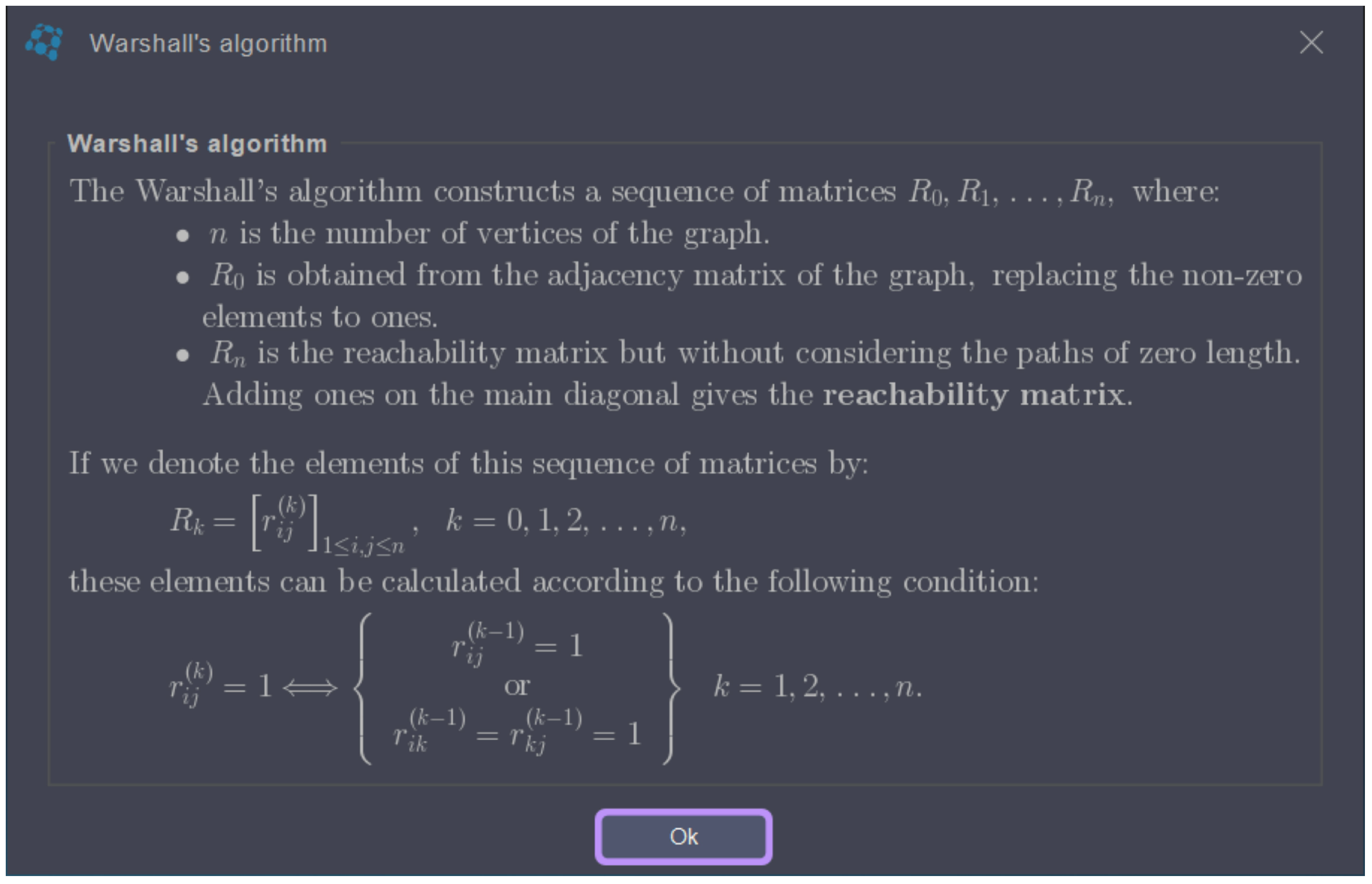
- View algorithms menu: This shows a detailed description of the algorithms included in the software.

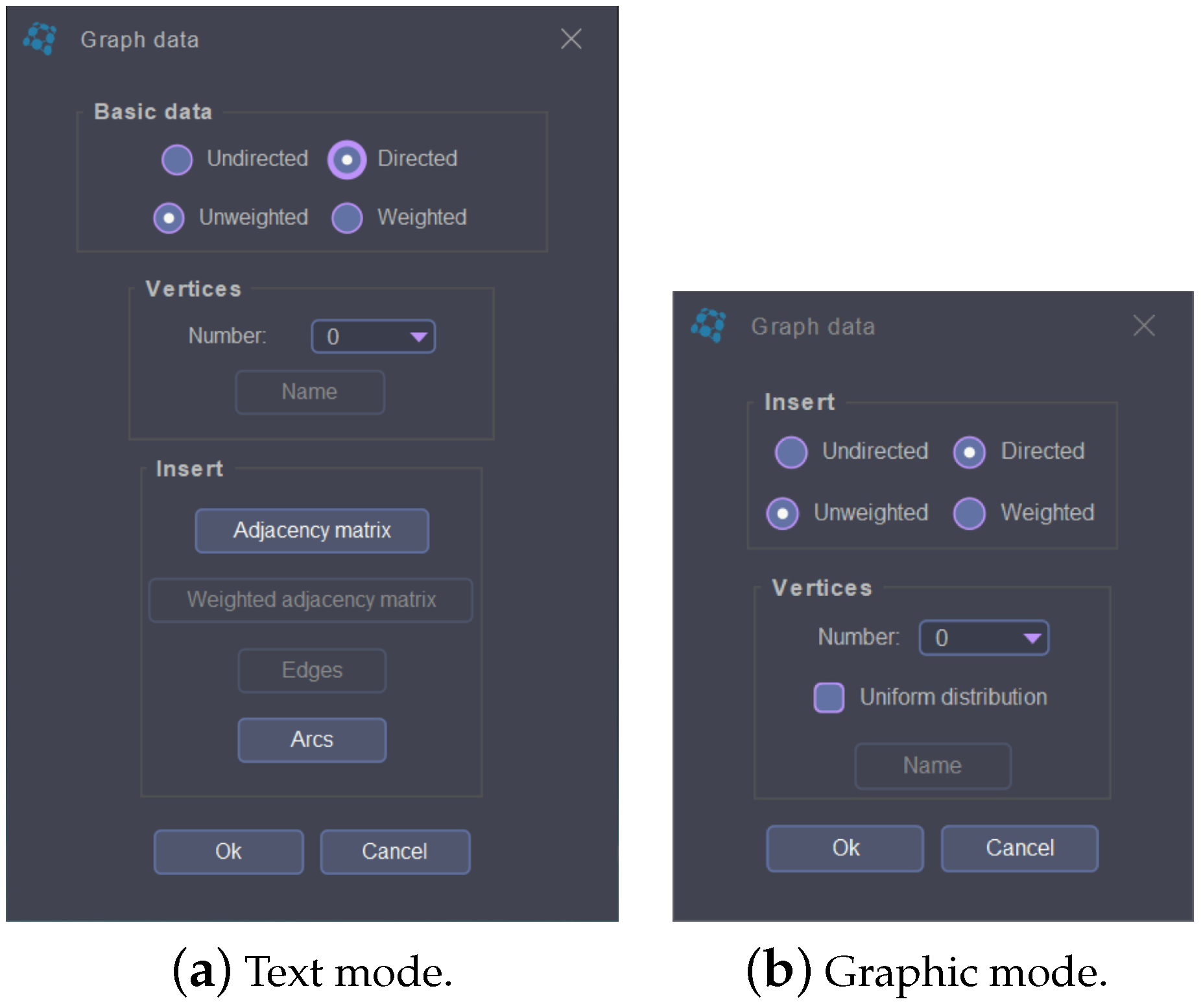
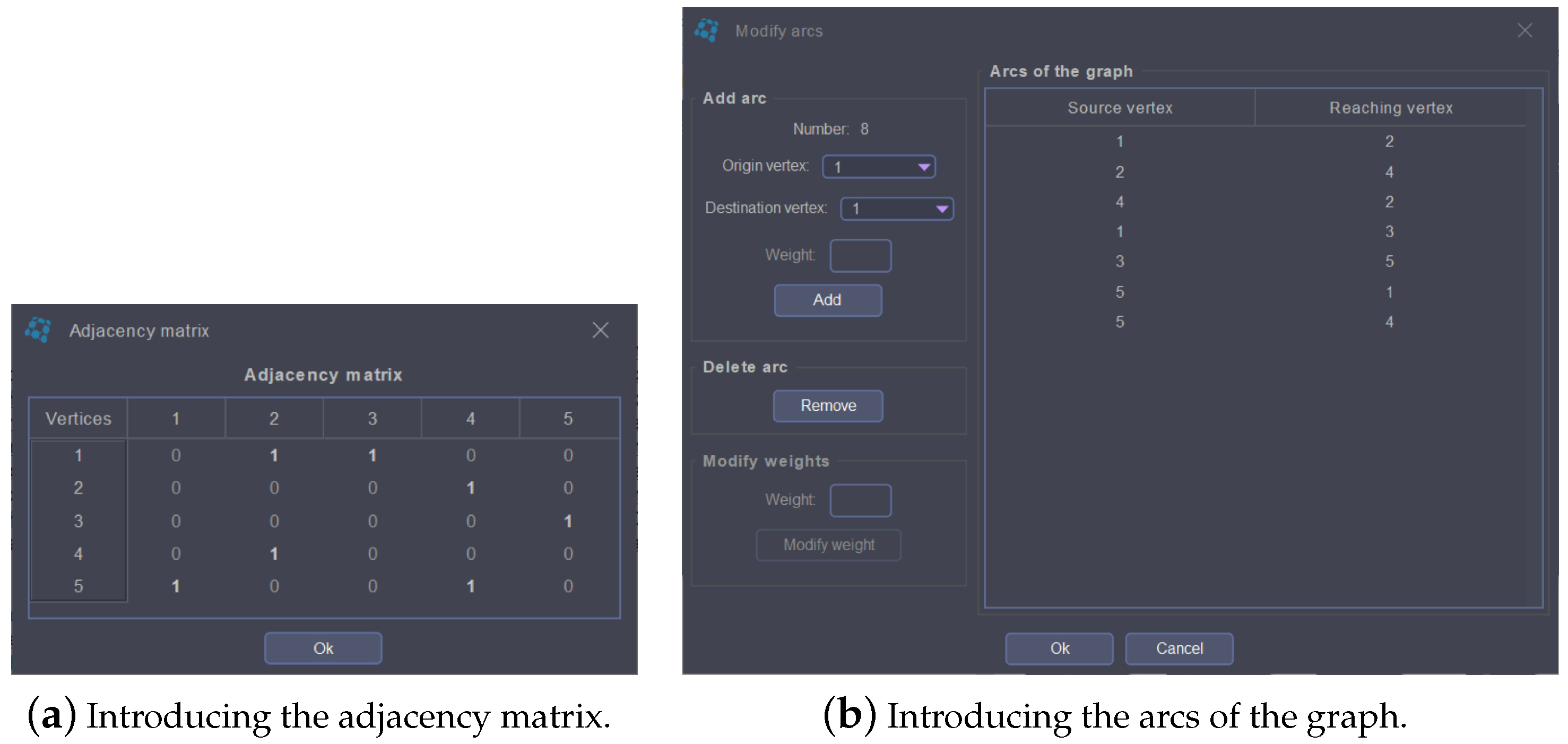
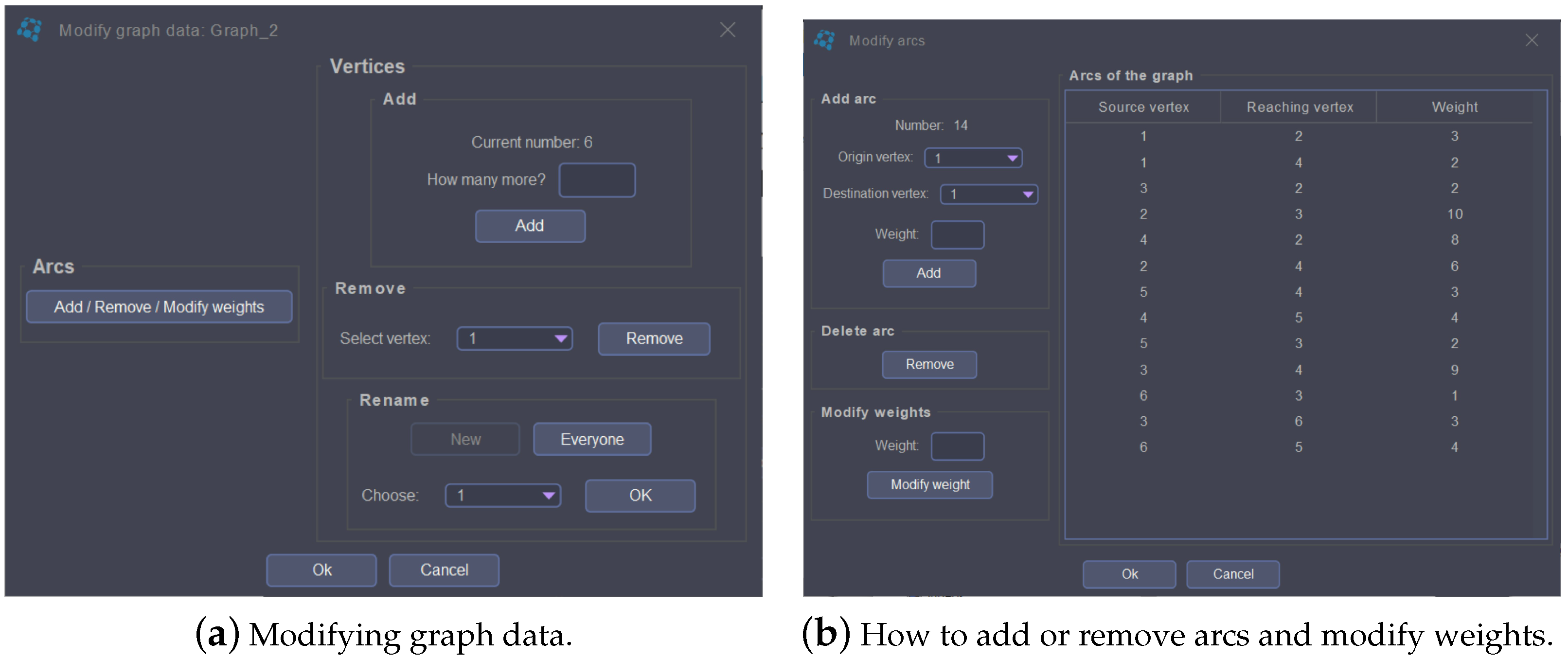
2.2.1. Graph Menu
2.2.2. Basic Calculations Menu
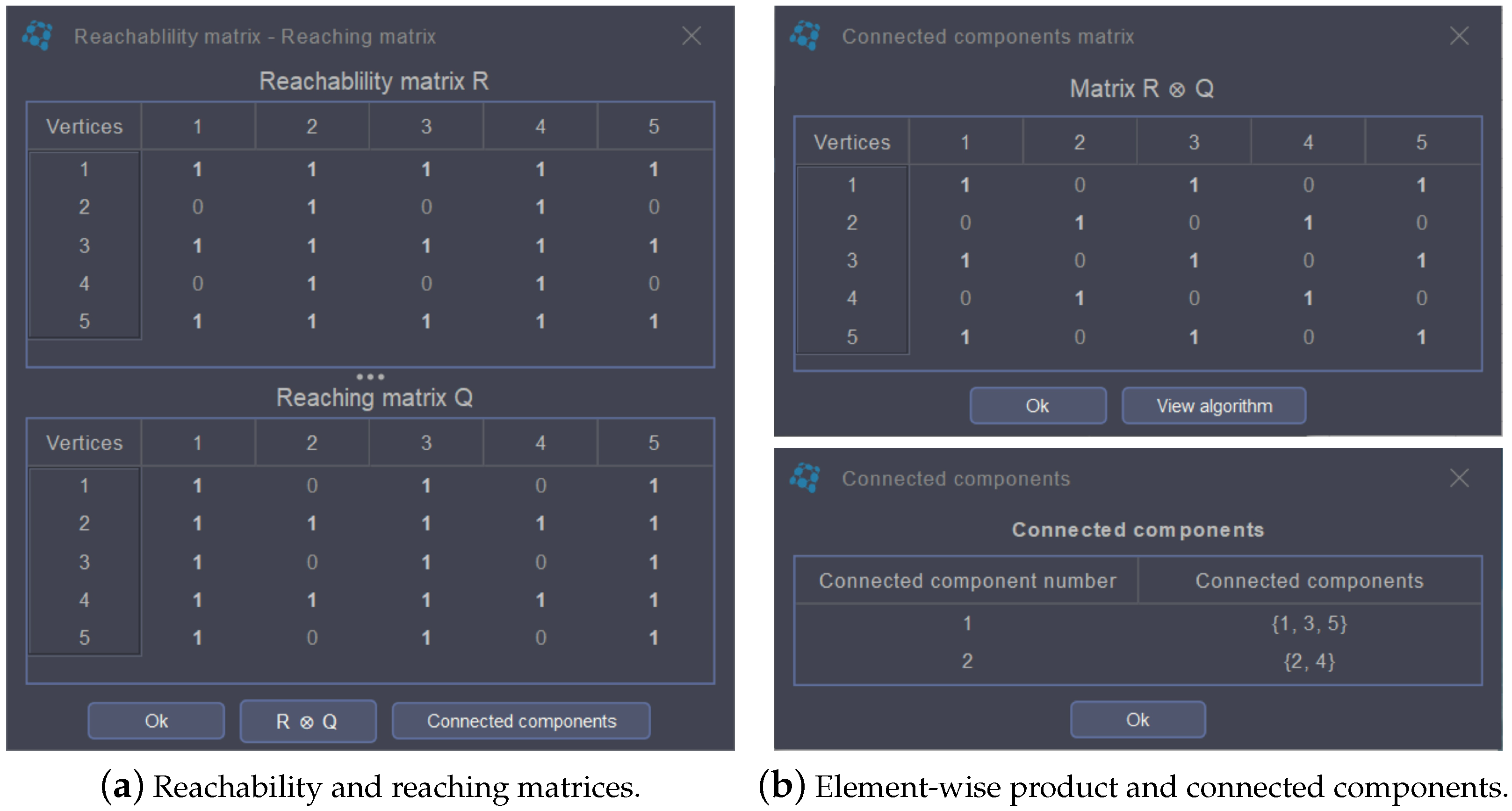
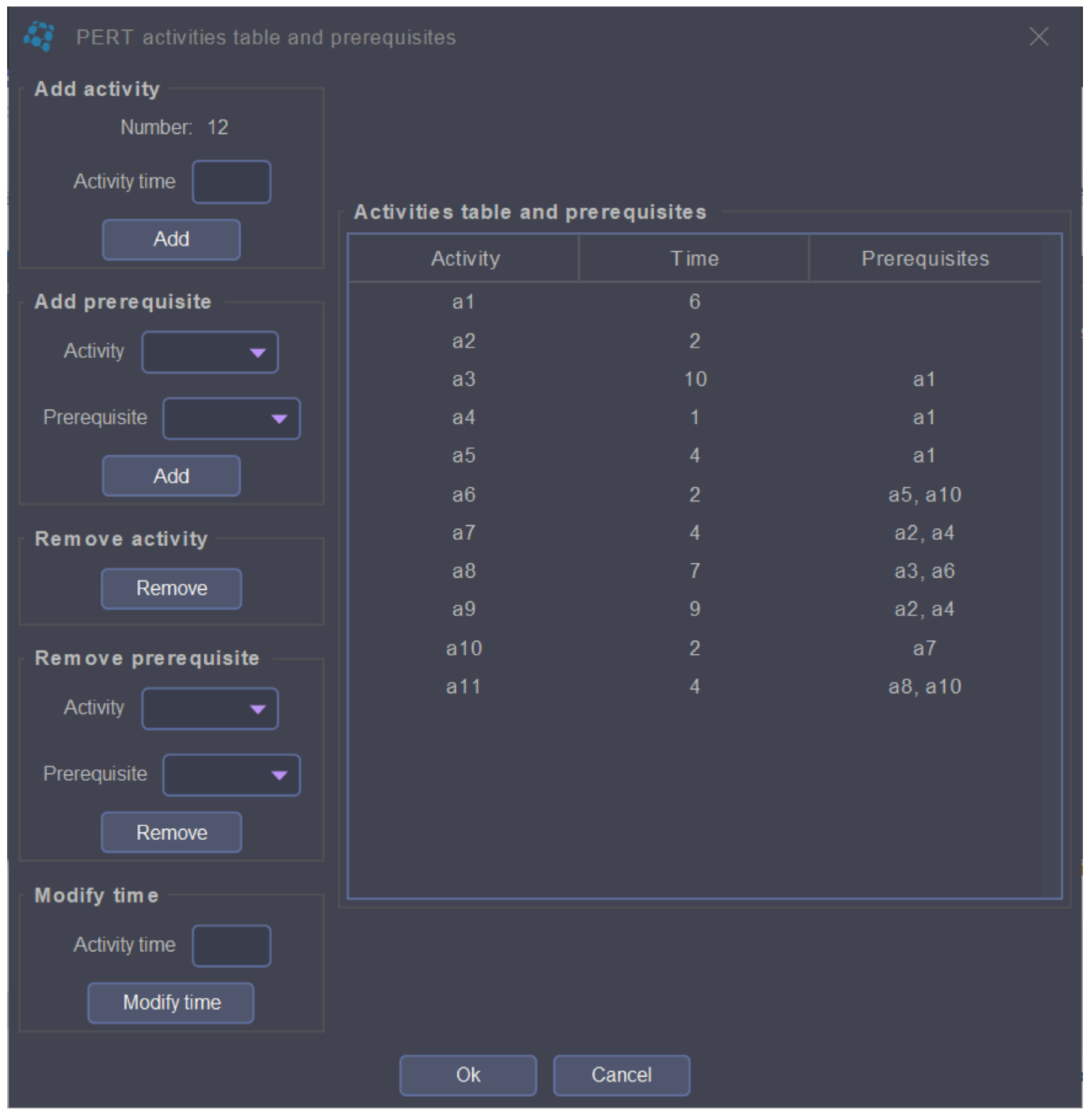
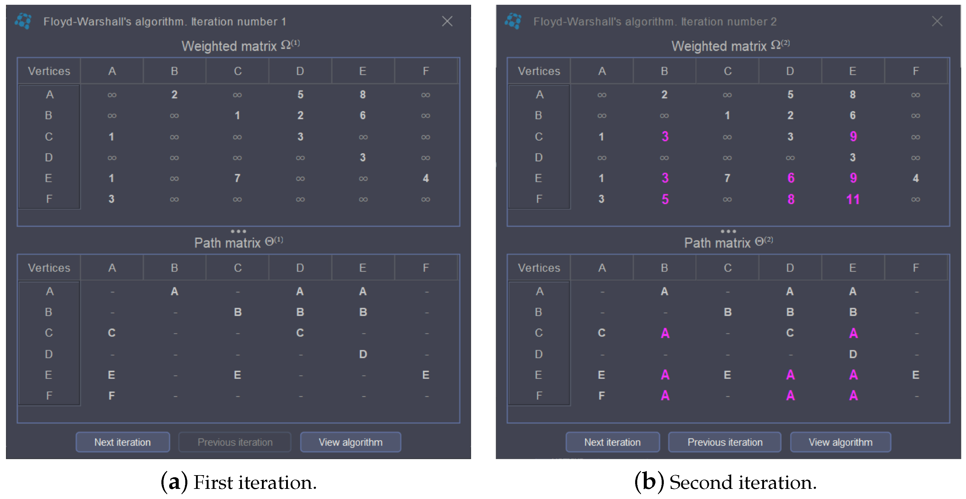
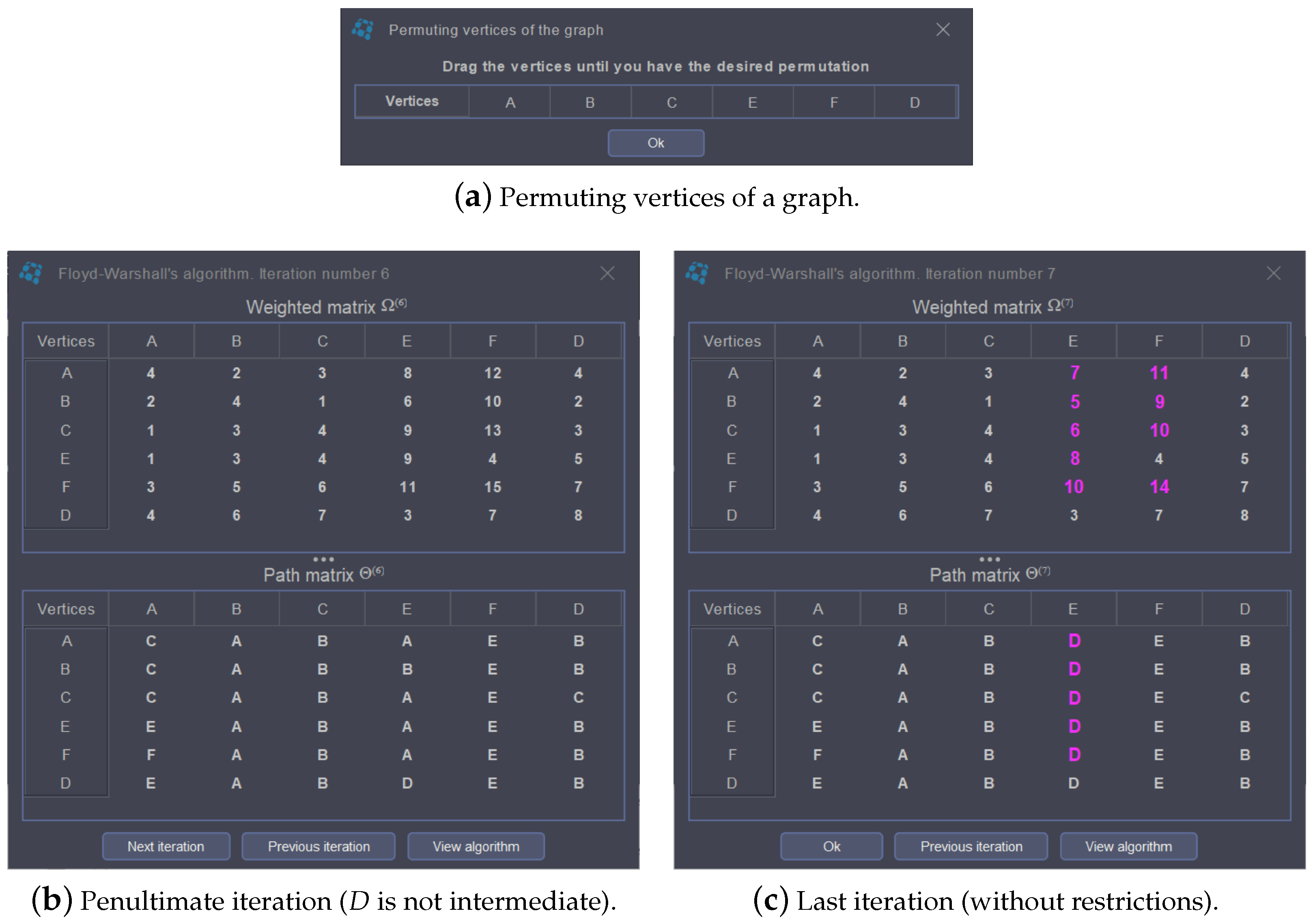
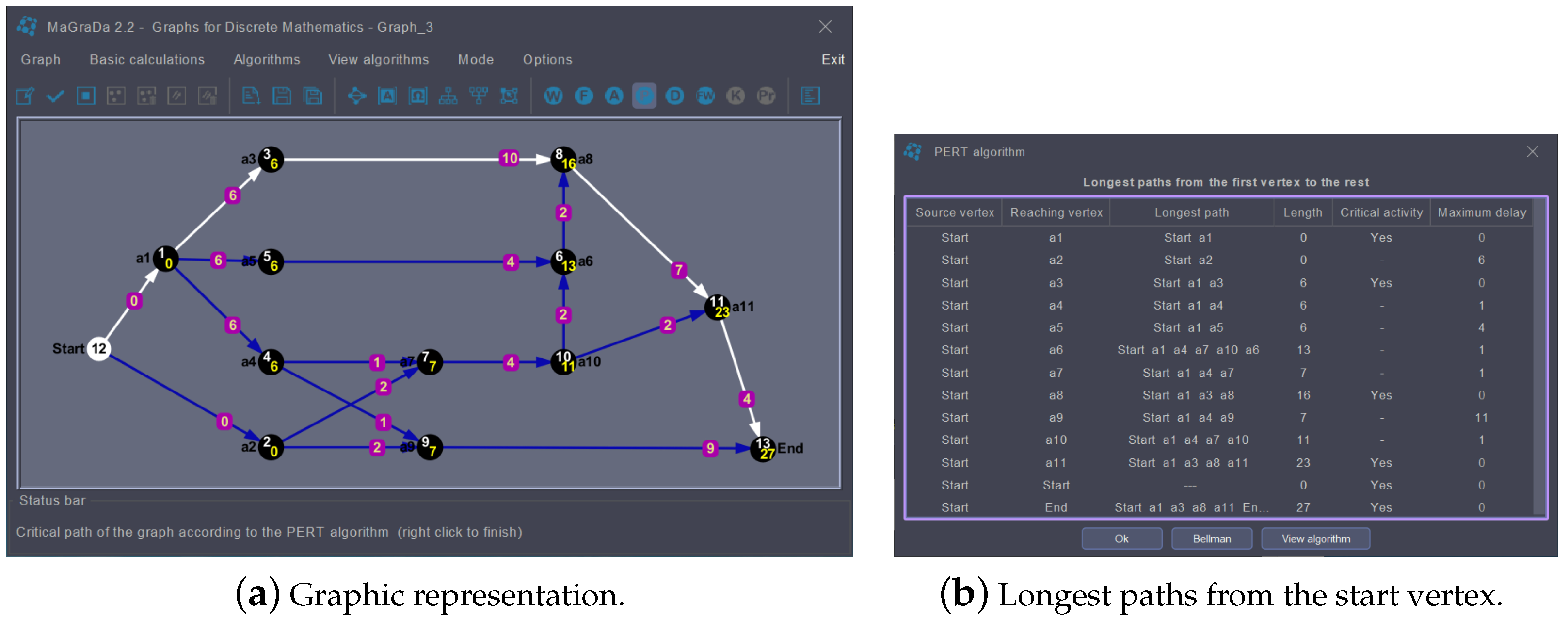
2.2.3. Algorithms and View Algorithms Menus
3. Materials and Methods
3.1. Description of the DM Course
3.2. Survey Overview and Reliability
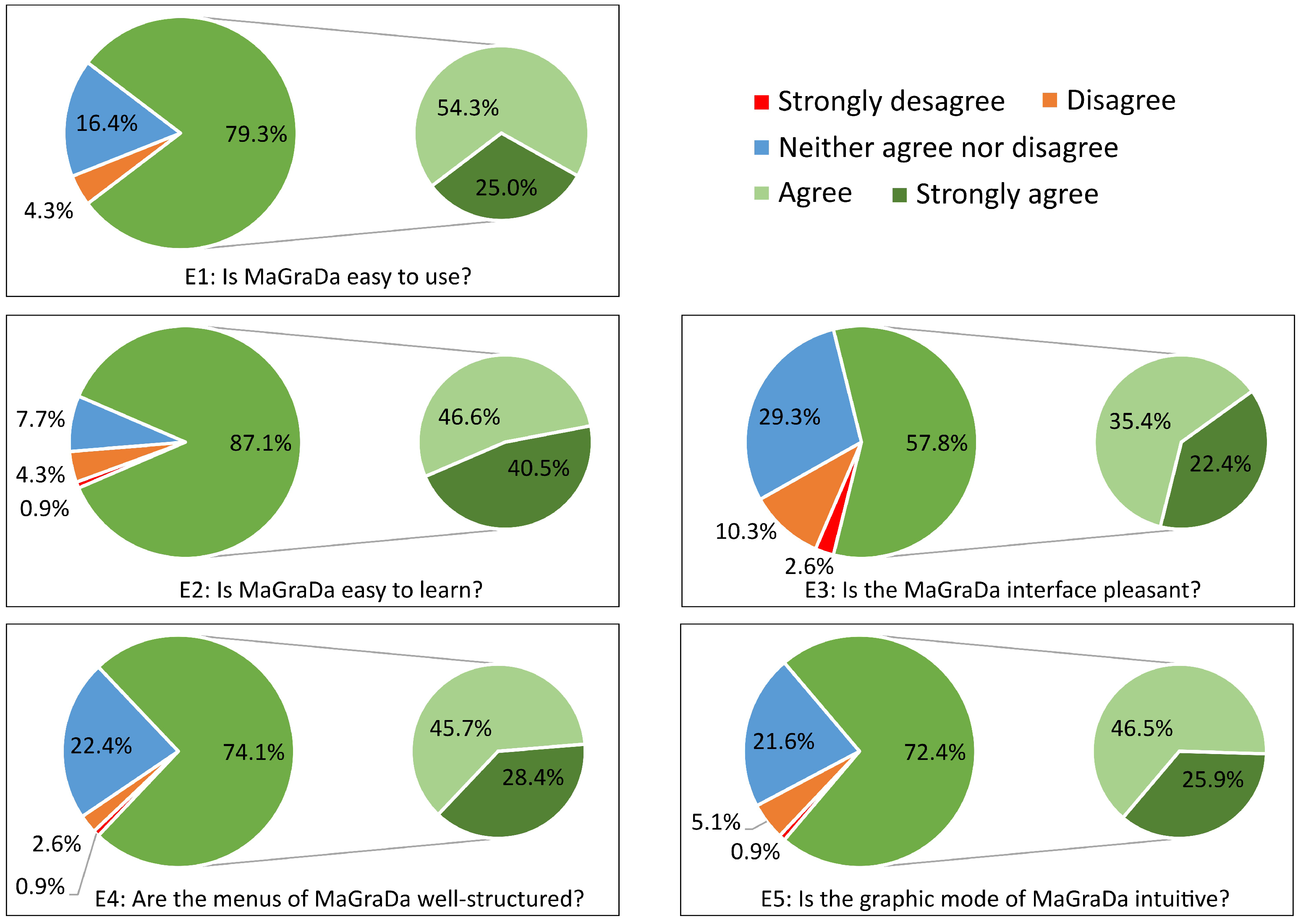
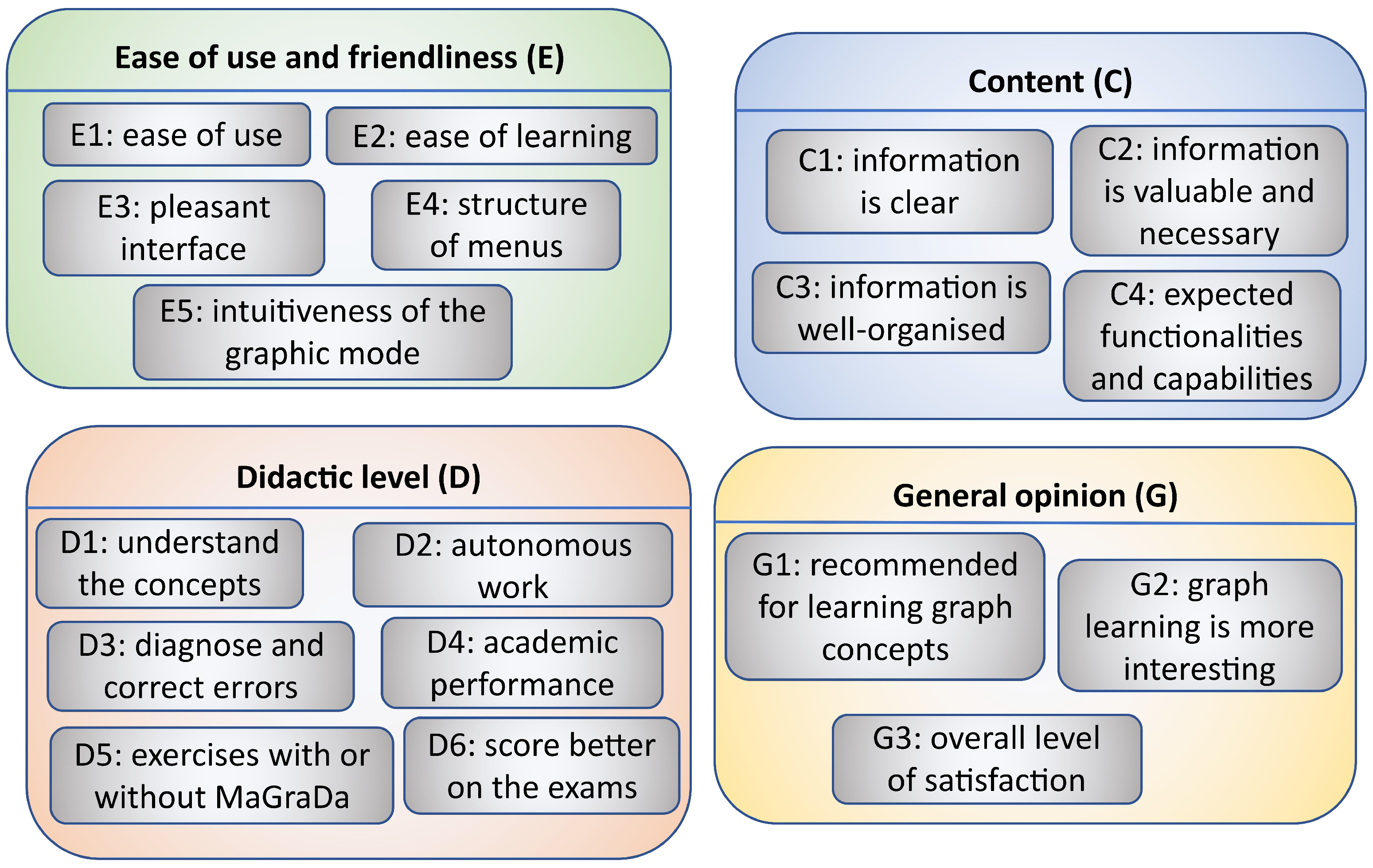
- Questions about the ease of use and friendliness of MaGraDa (E): the users answered questions about their level of satisfaction with the ease of use of MaGraDa (E1), the ease of learning the software (E2), the pleasantness of the interface (E3), the structure of the menus (E4) and the intuitiveness of the graphic mode (E5).
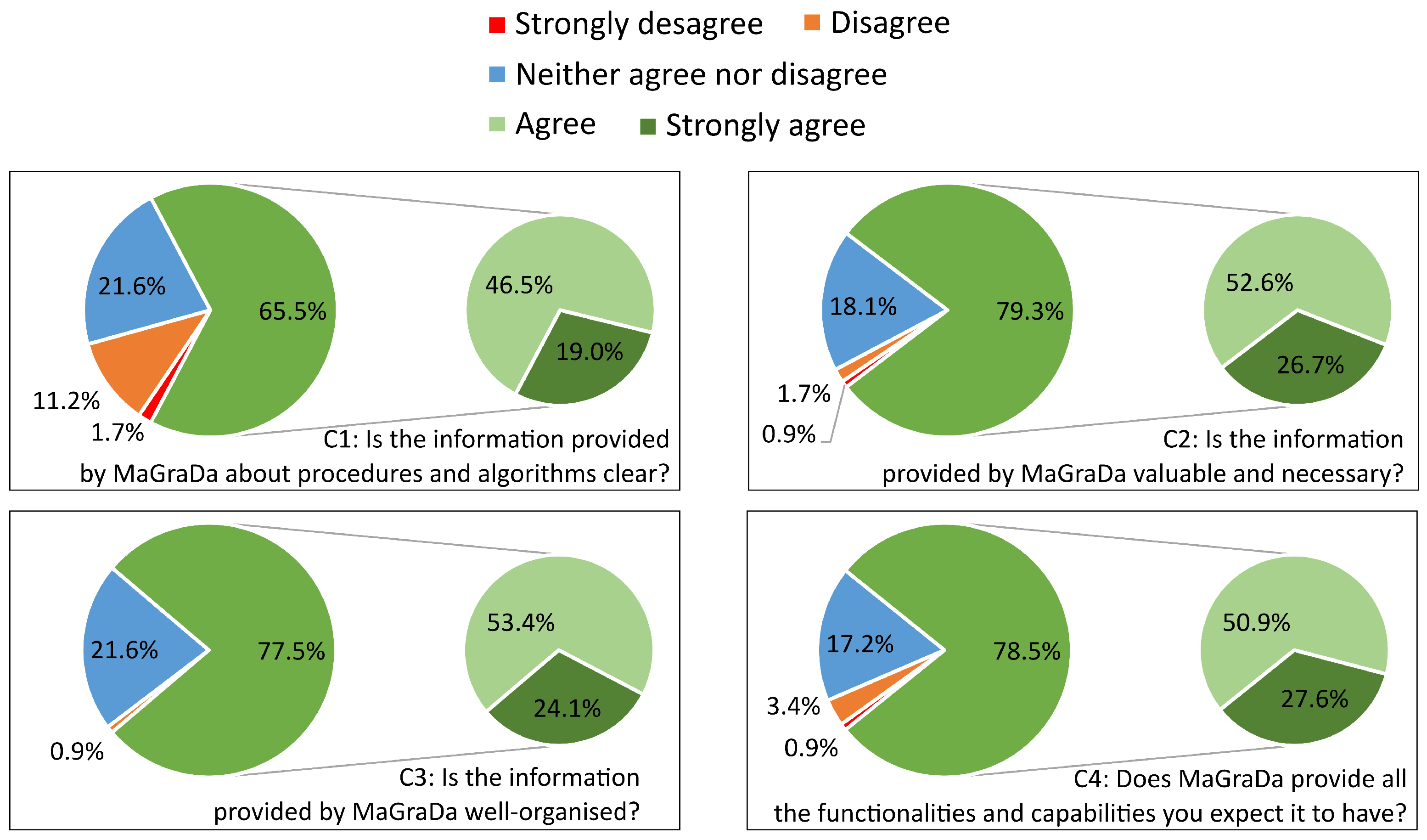
- Questions about the content of MaGraDa (C): these covered aspects related to the information provided by the procedures and algorithms (C1), the need for the information contained in MaGraDa (C2), its organisation (C3), and the functionalities and capabilities offered by MaGraDa (C4).
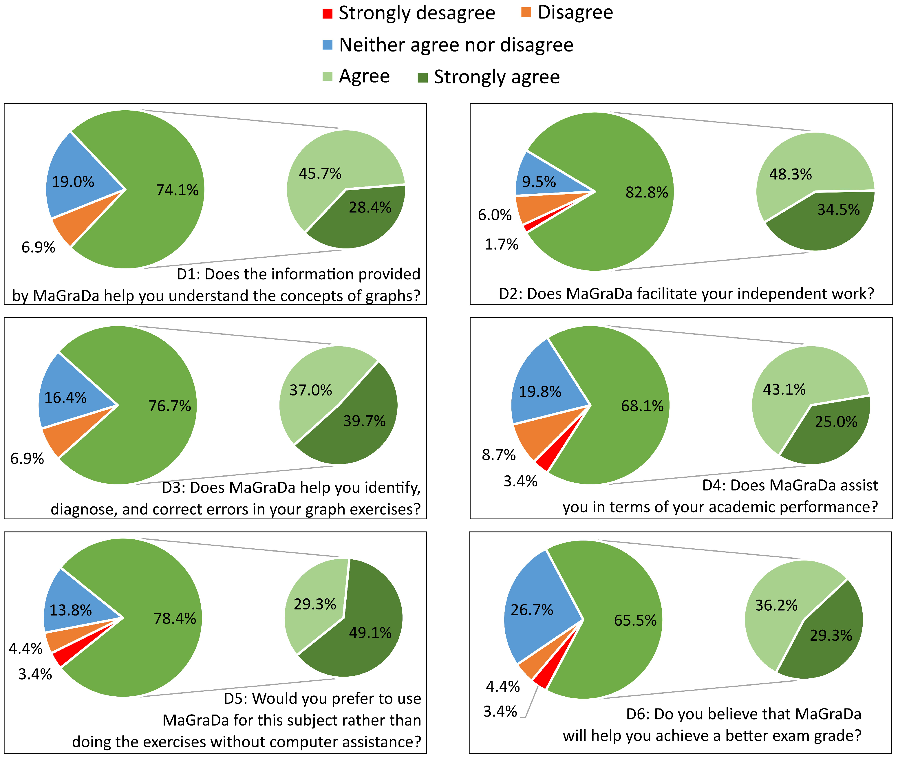
- Questions about the didactic level of MaGraDa (D): the users answered questions about whether MaGraDa helped them to understand the concepts of graphs (D1), whether MaGraDa facilitated independent work (D2), whether MaGraDa helped them to identify, diagnose and correct errors in their graph exercises (D3), whether MaGraDa helped them in terms of their academic performance (D4), whether they would prefer to use MaGraDa rather than performing the exercises without computer assistance (D5), and finally their opinions about the help that MaGraDa could provide in terms of scoring better on the exams (D6).
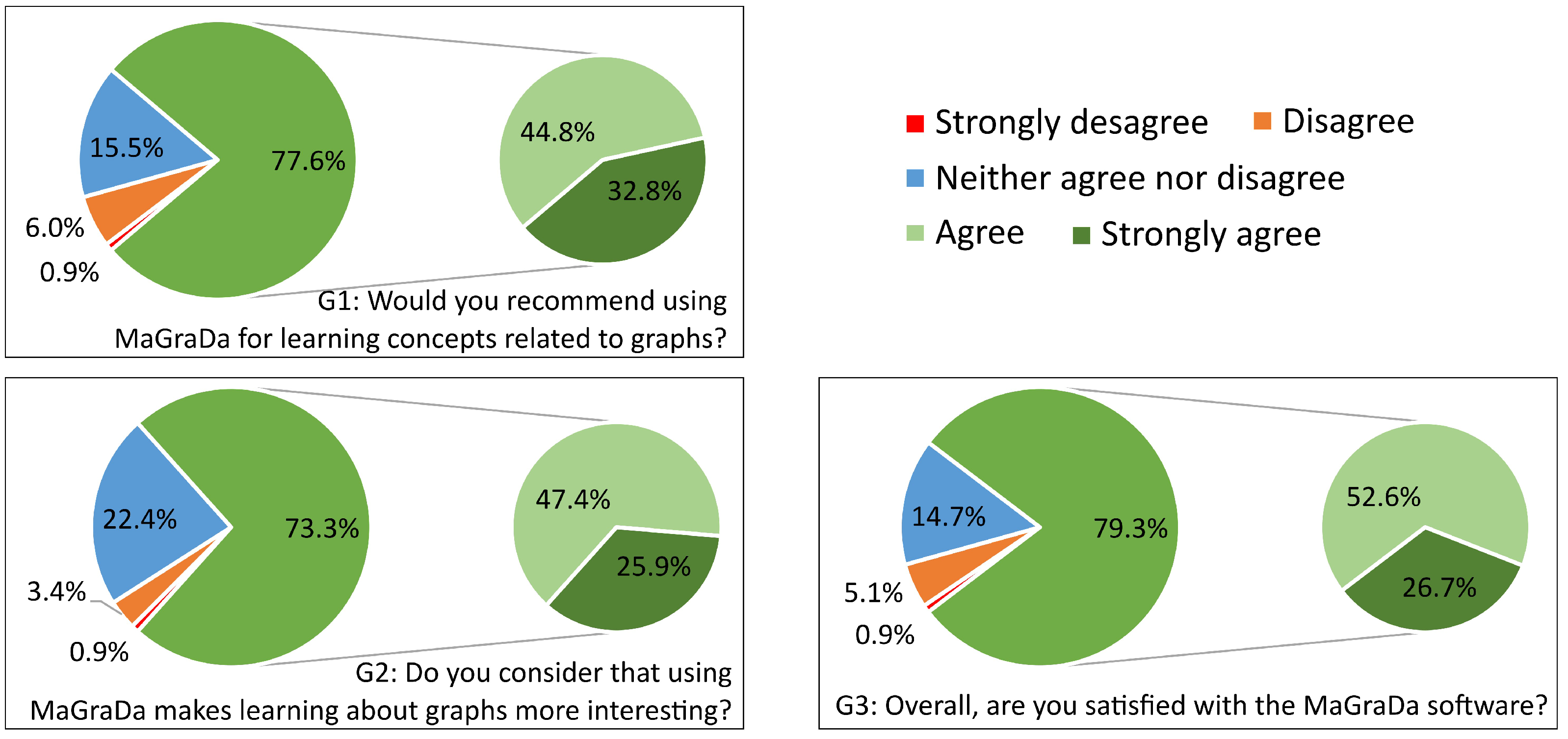
- Questions about general opinions on MaGraDa (G): three questions were included about whether they would recommend MaGraDa for learning concepts about graphs (G1), whether MaGraDa made learning about graphs more interesting (G2), and an overall question about their level of satisfaction with MaGraDa (G3).
4. Survey Exploratory Analysis
4.1. Exploratory Factor Analysis
4.2. Principal Component Analysis
4.3. Categorical Principal Component Analysis
5. Survey Results, Analysis and Discussion
6. Conclusions
Author Contributions
Funding
Informed Consent Statement
Data Availability Statement
Acknowledgments
Conflicts of Interest
Abbreviations
| MaGraDa | Graphs for Discrete Mathematics |
| DM | Discrete Mathematics |
| GRIN | Graph Interface |
| GIRL | Graph Information Retrieval Language |
| GASP | Graph Algorithm Software Package |
| GTPL | Graph Theoretic Programming Language |
| IDE | Integrated Development Environment |
| STEM | Science, Technology, Engineering, and Mathematics |
| JDK | Java Development Kit |
| FlatLaf | Flat Look and Feel |
| JUNG | Java Universal Network/Graph |
| L&F | Look and Feel |
| PERT | Program Evaluation Review Technique |
| MLR | Multiple linear regression |
| KMO | Kaiser-Meyer-Olkin |
| FA | Factor analysis |
| PCA | Principal component analysis |
| EFA | Exploratory factor analysis |
| CFA | Confirmatory factor analysis |
| CATPCA | Categorical principal component analysis |
| PAF | Principal axis factoring |
| ANOVA | Analysis of variance |
References
- CC2020 Task Force. Computing Curricula 2020: Paradigms for Global Computing Education; ACM: New York, NY, USA, 2020. [Google Scholar] [CrossRef]
- Joint Task Force on Computing Curricula; ACM; IEEE Computer Society. Computer Science Curricula 2013: Curriculum Guidelines for Undergraduate Degree Programs in Computer Science; ACM: New York, NY, USA, 2013. [Google Scholar] [CrossRef]
- Veerarajan, T. Discrete Mathematics with Graph Theory and Combinatorics; Computer Science Series; McGraw-Hill: New York, NY, USA, 2006. [Google Scholar]
- Christofides, N. Graph Theory. An Algorithmic Approach; Academic Press: Cambridge, MA, USA, 1975. [Google Scholar]
- Dierker, P.F.; Voxman, W.L. Discrete Mathematics; Harcourt Brace Jovanovich: San Diego, CA, USA, 1986. [Google Scholar]
- Grimaldi, R.P. Discrete and Combinatorial Mathematics. An Applied Introduction; Addison-Wesley: Boston, MA, USA, 2003. [Google Scholar]
- Joint Task Force on Computer Engineering Curricula; ACM; IEEE Computer Society. Computer Engineering Curricula 2016: Curriculum Guidelines for Undergraduate Degree Programs in Computer Engineering; ACM: New York, NY, USA, 2016; Available online: https://www.acm.org/binaries/content/assets/education/ce2016-final-report.pdf (accessed on 10 May 2023).
- ACM Data Science Task Force. Computing Competencies for Undergraduate Data Science Curricula; ACM: New York, NY, USA, 2021. [Google Scholar] [CrossRef]
- Task Group on Information Technology Curricula. Information Technology Curricula 2017: Curriculum Guidelines for Baccalaureate Degree Programs in Information Technology; ACM: New York, NY, USA, 2017. [Google Scholar] [CrossRef]
- Joint Task Force on Computing Curricula; ACM; IEEE Computer Society. Curriculum Guidelines for Undergraduate Degree Programs in Software Engineering; ACM: New York, NY, USA, 2014. [Google Scholar]
- Flegg, J.; Mallet, D.; Lupton, M. Students’ perceptions of the relevance of mathematics in engineering. Int. J. Math. Educ. Sci. Technol. 2012, 43, 717–732. [Google Scholar] [CrossRef]
- Gueudet, G.; Quéré, P. “Making connections” in the mathematics courses for engineers: The example of online resources for trigonometry. In Proceedings of the Second Conference of the International Network for Didactic Research in University Mathematics; INDRUM2018; Durand-Guerrier, V., Hochmuth, R., Goodchild, S., Hogstad, N.M., Eds.; University of Agder and INDRUM: Kristiansand, Norway, 2018. [Google Scholar]
- Majeed, A.; Rauf, I. Graph Theory: A Comprehensive Survey about Graph Theory Applications in Computer Science and Social Networks. Inventions 2020, 5, 10. [Google Scholar] [CrossRef]
- Campbell, W.M.; Dagli, C.K.; Weinstein, C.J. Social Network Analysis with Content and Graphs. Linc. Lab. J. 2013, 20, 62–81. [Google Scholar]
- Tabchi, T.; Sabra, H.; Ouvrier-Buffet, C. Resources for teaching graph theory for engineers—Issue of connectivity. In Proceedings of the 3rd International Conference on Mathematics Textbook Research and Development; Rezat, S., Fan, L., Hattermann, M., Schumacher, J., Wuschke, H., Eds.; Universitätsbibliothek Paderborn: Paderborn, Germany, 2019; pp. 323–328. [Google Scholar]
- Gamage, S.H.P.W.; Ayres, J.R.; Behrend, M.B. A systematic review on trends in using Moodle for teaching and learning. Int. J. STEM Educ. 2022, 9, 9. [Google Scholar] [CrossRef] [PubMed]
- Carbonneaux, Y.; Laborde, J.M.; Madani, R.M. CABRI-Graph: A tool for research and teaching in graph theory. In Graph Drawing; Lecture Notes in Computer, Science; Brandenburg, F.J., Ed.; Springer: Berlin/Heidelberg, Germany, 1996; Volume 1027, pp. 123–126. [Google Scholar] [CrossRef]
- Baudon, O.; Laborde, J. Cabri-graph, a sketchpad for graph theory. Math. Comput. Simul. 1996, 42, 765–774. [Google Scholar] [CrossRef]
- Schliep, A.; Hochstättler, W. Developing Gato and CATBox with Python: Teaching graph algorithms through visualization and experimentation. In Multimedia Tools for Communicating Mathematics; Mathematics and, Visualization; Borwein, J., Morales, M.H., Rodrigues, J.F., Polthier, K., Eds.; Springer: Berlin/Heidelberg, Germany, 2002; pp. 291–309. [Google Scholar] [CrossRef]
- Lambert, A.; Auber, D. Graph analysis and visualization with Tulip-Python. In Proceedings of the EuroSciPy 2012—5th European meeting on Python in Science, Brussels, Belgium, 23–27 August 2012. [Google Scholar]
- Rostami, M.A.; Azadi, A.; Seydi, M. GraphTea: Interactive graph self-teaching tool. In Communications, Circuits and Educational Technologies: 2014 International Conference on Education and Educational Technologies II (EET’14); Wseas Llc Staff: Prague, Czech Republic, 2014; pp. 48–51. [Google Scholar]
- Rodríguez-Villalobos, A. Grafos. Available online: https://arodrigu.webs.upv.es/grafos/doku.php (accessed on 15 September 2023).
- Pechenkin, V. GRIN (GRaph INterface). 2022. Available online: https://grin-software.net (accessed on 15 September 2023).
- Neo4j Connections: Generative AI and Knowledge Graphs. 2010. Available online: https://neo4j.com (accessed on 26 November 2023).
- Gremlin Query Language. 2009. Available online: https://tinkerpop.apache.org/gremlin.html (accessed on 26 November 2023).
- Ševčíková, A.; Milková, E. Multimedia applications: Graph algorithms visualization. In Proceedings of the 2016 IEEE 17th International Symposium on Computational Intelligence and Informatics (CINTI), Budapest, Hungary, 17–19 November 2016; pp. 231–236. [Google Scholar] [CrossRef]
- Sevcikova, A.; Milkova, E.; Moldoveanu, M.; Konvicka, M. Graph Theory: Enhancing Understanding of Mathematical Proofs Using Visual Tools. Sustainability 2023, 15, 10536. [Google Scholar] [CrossRef]
- Dagdilelis, V.; Satratzemi, M. DIDAGRAPH: Software for teaching graph theory algorithms. ACM SIGCSE Bull. 1998, 30, 64–68. [Google Scholar] [CrossRef]
- Hawick, K. Interactive Graph Algorithm Visualization and the GraViz Prototype; Technical Report CSTN-061; Institute of Information and Mathematical Sciences, Massey University: Auckland, New Zealand, 2010. [Google Scholar]
- Chaudhary, P.; Kumar, V. A Review on Applications of Graph Theory in Computer Science. J. Adv. Sci. Tecnol. 2020, 17, 82–87. [Google Scholar]
- Rodgers, P.J.; Vidal, N. Graph algorithm animation with Grrr. In Proceedings of the Applications of Graph Transformations with Industrial Relevance; Nagl, M., Schürr, A., Münch, M., Eds.; Springer: Berlin/Heidelberg, Germany, 2000; pp. 379–394. [Google Scholar] [CrossRef]
- Caballero, M.; Migallón, V.; Penadés, J. MaGraDa: Una Herramienta para el tratamiento de grafos en matemática discreta. In Proceedings of the VII Jornadas de Enseñanza Universitaria de la Informática; Miró, J., Ed.; Universitat de les Illes Balears: Palma de Mallorca, Spain, 2001; pp. 478–481. [Google Scholar]
- Rosen, K.H. Discrete Mathematics and Its Applications; McGraw-Hill: New York, NY, USA, 1999. [Google Scholar]
- JLaTeXMath—A Java API to Render LaTeX—A Java Package to Display LaTeX Code in Mathematical Mode. 2021. Available online: https://github.com/opencollab/jlatexmath. (accessed on 3 September 2023).
- FlatLaf—Flat Look and Feel. 2022. Available online: https://www.formdev.com/flatlaf/ (accessed on 3 September 2023).
- JUNG (Java Universal Network/Graph). 2009. Available online: https://jung.sourceforge.net/doc/index.html (accessed on 3 September 2023).
- O’Madadhain, J.; Fisher, D.; Smyth, P.; White, S.; Boey, Y.B. Analysis and visualization of network data using JUNG. J. Stat. Softw. 2005, 10, 1–35. [Google Scholar] [CrossRef]
- Mittelbach, F.; Goossens, M.; Braams, J.; Carlisle, D.; Rowley, C. The LaTeX Companion, 2nd ed.; Pearson Education, Inc.: Boston, MA, USA, 2004. [Google Scholar]
- Brandes, U.; Eiglsperger, M.; Herman, I.; Himsolt, M.; Marshall, M.S. GraphML progress report structural layer proposal. In Proceedings of the Graph Drawing; Mutzel, P., Jünger, M., Leipert, S., Eds.; Springer: Berlin/Heidelberg, Germany, 2002; pp. 501–512. [Google Scholar] [CrossRef]
- Grassmann, W.K.; Tremblay, J.P. Logic and Discrete Mathematics: A Computer Science Perspective; Prentice-Hall: Upper Saddle River, NJ, USA, 1996. [Google Scholar]
- W3C. Extensible Markup Language (XML) 1.0. 2008. Available online: https://www.w3.org/TR/xml/ (accessed on 3 September 2023).
- Gephi—The Open Graph Viz Platform. 2008. Available online: https://gephi.org/ (accessed on 3 September 2023).
- yEd—Graph Editor. 2023. Available online: https://www.yworks.com/products/yed (accessed on 3 September 2023).
- Gross, J.L.; Yellen, J. Graph Theory and Its Applications; CRC Press: Boca Raton, FL, USA, 2006. [Google Scholar]
- Aho, A.V.; Alspach, B.; Archdeacon, D.; Arney, D.C.; Balbuena, C.; Beineke, L.W.; Blazewicz, J.; Bollobás, B.; Bonato, A.; Bonchev, D.; et al. Handbook of Graph Theory; Gross, J.L., Yellen, J., Zhang, P., Eds.; CRC Press: Boca Raton, FL, USA, 2013. [Google Scholar] [CrossRef]
- Migallón, V.; Penadés, J. Matemática Discreta; Puntero y Chip: Alicante, Spain, 2004. [Google Scholar]
- Secretary-General of the OECD. The Impact of COVID-19 On Education: Insights from Education at a Glance 2020. Available online: https://www.oecd.org/education/the-impact-of-covid-19-on-education-insights-education-at-a-glance-2020.pdf (accessed on 10 September 2023).
- Likert, R. A Technique for the Measurement of Attitudes. Arch. Psychol. 1932, 22, 5–55. [Google Scholar]
- Batterton, K.A.; Hale, K.N. The Likert Scale What It Is and How To Use It. Phalanx 2017, 50, 32–39. [Google Scholar]
- IBM Corp. IBM SPSS Statistics for Windows. 2023. Available online: https://www.ibm.com/uk-en/analytics/spss-statistics-software (accessed on 20 May 2023).
- Hardy, M.A. Regression with Dummy Variables; Sage University Paper Series on Quantitative Applications in the Social Science, 07-093; Sage: Newbury Park, CA, USA, 1993. [Google Scholar]
- Wang, F. Factor analysis and principal-components analysis. In International Encyclopedia of Human Geography, 2nd ed.; Kobayashi, A., Ed.; Elsevier: Oxford, UK, 2009; pp. 1–7. [Google Scholar] [CrossRef]
- Linting, M.; Meulman, J.J.; Groenen, P.J.; van der Koojj, A.J. Nonlinear principal components analysis: Introduction and application. Psychol. Methods 2007, 12, 336–358. [Google Scholar] [CrossRef] [PubMed]
- Cronbach, L.J. Coefficient alpha and the internal structure of tests. Psychometrika 1951, 16, 297–334. [Google Scholar] [CrossRef]
- Tavakol, M.; Dennick, R. Making sense of Cronbach’s alpha. Int. J. Med. Educ. 2011, 2, 53. [Google Scholar] [CrossRef] [PubMed]
- Norman, G. Likert scales, levels of measurement and the “law” of statistics. Adv. Health Sci. Educ. 2010, 15, 625–632. [Google Scholar] [CrossRef] [PubMed]
- MacCallum, R.C.; Widaman, K.F.; Zhang, S.; Hong, S. Sample size in factor analysis. Psychol. Methods 1999, 4, 84–89. [Google Scholar] [CrossRef]
- Shrestha, N. Factor Analysis as a Tool for Survey Analysis. Am. J. Appl. Math. 2021, 9, 4–11. [Google Scholar] [CrossRef]
- Pearson, E.S. The Test of Significance for the Correlation Coefficient. J. Am. Stat. Assoc. 1931, 26, 128–134. [Google Scholar] [CrossRef]
- Pearson, E.S. The Test of Significance for the Correlation Coefficient: Some Further Results. J. Am. Stat. Assoc. 1932, 27, 424–426. [Google Scholar] [CrossRef]
- Havlicek, L.L.; Peterson, N.L. Robustness of the Pearson correlation against violations of assumptions. Percept. Mot. Skills 1976, 43, 1319–1334. [Google Scholar] [CrossRef]
- Fletcher, K.E.; French, C.T.; Irwin, R.S.; Corapi, K.M.; Norman, G.R. A prospective global measure, the Punum Ladder, provides more valid assessments of quality of life than a retrospective transition measure. J. Clin. Epidemiol. 2010, 63, 1123–1131. [Google Scholar] [CrossRef] [PubMed]


| Topic | Content |
|---|---|
| Fundamentals of graphs | Definition and graph terminology. Special types of graphs. Vertex degree. Paths and connectedness. Graph isomorphism. Matrix representations. |
| Accessibility and connectivity | Accessibility. Warshall algorithm. Computation of connected components. Euler paths and Euler tours. Fleury algorithm. Hamiltonian paths and Hamiltonian cycles. Gray codes. |
| Trees | Definitions, properties, and examples. Rooted trees. Tree traversal. Polish notation. |
| Weighted graphs | Definition and examples. Shortest paths. Bellman equations. Acyclic graphs. Critical path method. Project Evaluation and Review Technique (PERT). Dijkstra shortest-path algorithm. Floyd-Warshall method. Minimum spanning trees. Kruskal and Prim algorithms. |
| Activity | Objectives |
|---|---|
| Introduction to MaGraDa | Exploring graph creation and manipulation from text and graphic modes of MaGraDa. Learning basic graph terminology and types. |
| Fundamentals of graphs | Learning concepts of graphs. Familiarisation with terminology related to graphs and how to apply the relationship between the degree of the vertices and the number of edges. Understanding the concept of graph isomorphism. Learning how to build the adjacency matrix and how to use it to calculate the degree of a vertex and the number of walks between two vertices. Learning how to build the incidence matrix and exploring its properties. |
| Accessibility and connectivity | Understanding the concepts of reachable and reaching vertices. Knowing how to apply the Warshall algorithm to obtain the reachability matrix. Knowing how to interpret the reachability and reaching matrices. Learning to calculate the connected components of a graph. Understanding the concepts of cutting-edge and cutting-vertex and their importance in some applications. |
| Euler paths and tours; Hamilton paths and cycles | Knowing how to reason about whether a graph is Eulerian, has an Eulerian path, or neither. Knowing how to build Eulerian paths and tours using the Fleury algorithm. Understanding the properties that allow us to reason about the existence or otherwise of Hamiltonian paths and cycles. |
| Introduction to the tree structure | Understanding the concepts of tree, spanning tree and rooted tree. Knowing how to apply some properties of trees. Learning how to build the Polish notations from the rooted tree of a mathematical expression and vice versa. |
| Weighted graphs; shortest paths in acyclic graphs | Knowing how to calculate the weighted adjacency matrix of a weighted graph. Learning how to use the Bellman equations to obtain shortest paths and critical paths in acyclic graphs. Exploring the utility of PERT. |
| Shortest paths | Identifying a shortest path problem based on a real-life situation. Addressing a shortest path problem using the Dijkstra and Floyd-Warshall algorithms. |
| Minimum spanning trees | Identifying a minimum spanning tree problem based on a real-life situation. Addressing a minimum spanning tree problem using the Kruskal and Prim algorithms. |
| Block | Variable Name | Question |
|---|---|---|
| Socio-demographic | SD1 | Age |
| SD2 | Gender | |
| SD3 | Highest university year | |
| SD4 | First time enrolling on the DM course | |
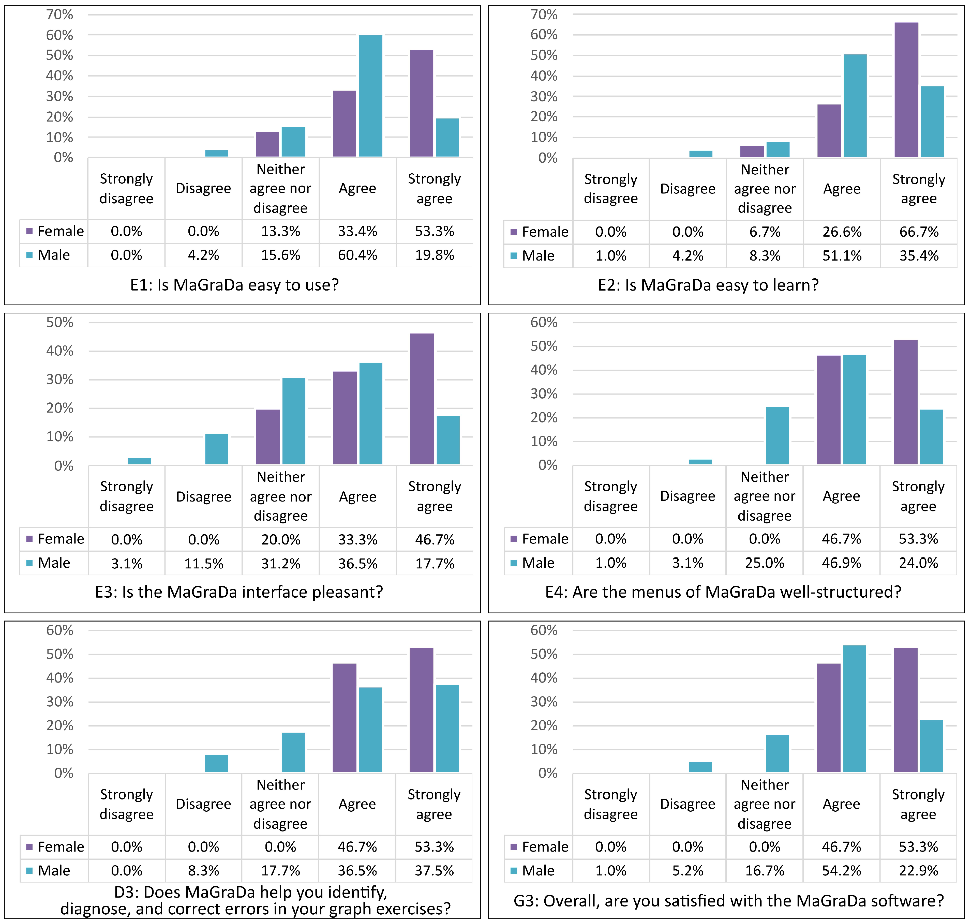
| Ease of use and friendliness | E1 | Is MaGraDa easy to use? |
| E2 | Is MaGraDa easy to learn? | |
| E3 | Is the MaGraDa interface pleasant? | |
| E4 | Are the menus of MaGraDa well-structured? | |
| E5 | Is the graphic mode of MaGraDa intuitive? | |
| Content | C1 | Is the information provided by MaGraDa about procedures and algorithms clear? |
| C2 | Is the information provided by MaGraDa valuable and necessary? | |
| C3 | Is the information provided by MaGraDa well-organised? | |
| C4 | Does MaGraDa provide all the functionalities and capabilities you expect it to have? | |
| Didactic level | D1 | Does the information provided by MaGraDa help you understand the concepts of graphs? |
| D2 | Does MaGraDa facilitate your independent work? | |
| D3 | Does MaGraDa help you identify, diagnose, and correct errors in your graph exercises? | |
| D4 | Does MaGraDa assist you in terms of your academic performance? | |
| D5 | Would you prefer to use MaGraDa for this subject rather than doing the exercises without computer assistance? | |
| D6 | Do you believe that MaGraDa will help you achieve a better exam grade? | |
| General opinion | G1 | Would you recommend using MaGraDa for learning concepts related to graphs? |
| G2 | Do you consider that using MaGraDa makes learning about graphs more interesting? | |
| G3 | Overall, are you satisfied with the MaGraDa software? | |
| Comments and suggestions | CS | Add any comments or suggestions about MaGraDa |
| Cronbach’s Alpha | Confidence Interval (95%) | Cronbach’s Alpha Based on Standardised Items | Number of Items |
|---|---|---|---|
| 0.894 | [0.864, 0.920] | 0.896 | 18 |
| Item | Scale Mean If Item Deleted | Scale Variance If Item Deleted | Corrected Item-Total Correlation | Squared Multiple Correlation | Cronbach’s Alpha If Item Deleted |
|---|---|---|---|---|---|
| E1 | 67.3621 | 83.816 | 0.516 | 0.561 | 0.889 |
| E2 | 67.1466 | 83.587 | 0.486 | 0.563 | 0.890 |
| E3 | 67.7155 | 80.744 | 0.537 | 0.444 | 0.888 |
| E4 | 67.3793 | 82.742 | 0.543 | 0.420 | 0.888 |
| E5 | 67.4483 | 87.449 | 0.213 | 0.297 | 0.898 |
| C1 | 67.6638 | 82.121 | 0.495 | 0.362 | 0.890 |
| C2 | 67.3362 | 82.347 | 0.621 | 0.517 | 0.886 |
| C3 | 67.3534 | 83.535 | 0.594 | 0.491 | 0.887 |
| C4 | 67.3534 | 83.622 | 0.494 | 0.414 | 0.889 |
| D1 | 67.4052 | 83.130 | 0.492 | 0.324 | 0.889 |
| D2 | 67.2845 | 81.962 | 0.536 | 0.461 | 0.888 |
| D3 | 67.2672 | 82.180 | 0.523 | 0.504 | 0.888 |
| D4 | 67.5862 | 79.845 | 0.585 | 0.592 | 0.886 |
| D5 | 67.1983 | 82.943 | 0.401 | 0.400 | 0.893 |
| D6 | 67.5259 | 80.043 | 0.586 | 0.608 | 0.886 |
| G1 | 67.3362 | 80.277 | 0.658 | 0.590 | 0.884 |
| G2 | 67.4224 | 80.750 | 0.680 | 0.621 | 0.884 |
| G3 | 67.3707 | 80.027 | 0.729 | 0.655 | 0.882 |
| KMO Measure of Sampling Adequacy | 0.877 |
| Bartlett test of sphericity (chi-square approximation) | 903.893 |
| Degrees of freedom | 153 |
| Significance |
| Initial Eigenvalues | Extraction Sums of Squared Loadings | Rotation Sums of Squared Loadings | |||||||
|---|---|---|---|---|---|---|---|---|---|
| Factor | Total | % of Variance | Cumulative % | Total | % of Variance | Cumulative % | Total | % of Variance | Cumulative % |
| 1 | 6.729 | 37.384 | 37.384 | 6.278 | 34.880 | 34.880 | 2.811 | 15.617 | 15.617 |
| 2 | 2.162 | 12.010 | 49.394 | 1.710 | 9.497 | 44.377 | 2.474 | 13.745 | 29.362 |
| 3 | 1.179 | 6.548 | 55.942 | 0.698 | 3.876 | 48.253 | 2.409 | 13.383 | 42.746 |
| 4 | 1.083 | 6.018 | 61.960 | 0.592 | 3.286 | 51.540 | 1.583 | 8.794 | 51.540 |
| 5 | 0.956 | 5.313 | 67.273 | ||||||
| 6 | 0.737 | 4.095 | 71.368 | ||||||
| 7 | 0.698 | 3.880 | 75.248 | ||||||
| 8 | 0.626 | 3.477 | 78.725 | ||||||
| 9 | 0.540 | 3.002 | 81.727 | ||||||
| 10 | 0.535 | 2.972 | 84.700 | ||||||
| 11 | 0.485 | 2.692 | 87.392 | ||||||
| 12 | 0.455 | 2.530 | 89.921 | ||||||
| 13 | 0.416 | 2.313 | 92.234 | ||||||
| 14 | 0.360 | 2.002 | 94.237 | ||||||
| 15 | 0.319 | 1.775 | 96.011 | ||||||
| 16 | 0.280 | 1.557 | 97.568 | ||||||
| 17 | 0.221 | 1.230 | 98.798 | ||||||
| 18 | 0.216 | 1.202 | 100.000 | ||||||
| Item | Factor 1 | Factor 2 | Factor 3 | Factor 4 |
|---|---|---|---|---|
| E1 | 0.106 | 0.755 | 0.063 | 0.244 |
| E2 | 0.026 | 0.705 | 0.067 | 0.356 |
| E3 | 0.194 | 0.417 | 0.168 | 0.452 |
| E4 | 0.250 | 0.221 | 0.180 | 0.603 |
| E5 | −0.019 | 0.139 | −0.043 | 0.551 |
| C1 | 0.144 | 0.302 | 0.316 | 0.321 |
| C2 | 0.391 | 0.180 | 0.597 | 0.077 |
| C3 | 0.122 | 0.170 | 0.547 | 0.498 |
| C4 | 0.022 | 0.391 | 0.385 | 0.288 |
| D1 | 0.292 | 0.295 | 0.285 | 0.130 |
| D2 | 0.624 | 0.214 | 0.166 | 0.070 |
| D3 | 0.708 | 0.108 | 0.142 | 0.114 |
| D4 | 0.800 | 0.070 | 0.208 | 0.117 |
| D5 | 0.296 | −0.043 | 0.477 | 0.089 |
| D6 | 0.656 | 0.010 | 0.449 | 0.044 |
| G1 | 0.391 | 0.375 | 0.592 | -0.047 |
| G2 | 0.278 | 0.526 | 0.558 | 0.025 |
| G3 | 0.383 | 0.539 | 0.413 | 0.154 |
| Initial Eigenvalues | Extraction Sums of Squared Loadings | Rotation Sums of Squared Loadings | |||||||
|---|---|---|---|---|---|---|---|---|---|
| Factor | Total | % of Variance | Cumulative % | Total | % of Variance | Cumulative % | Total | % of Variance | Cumulative % |
| 1 | 6.729 | 37.384 | 37.384 | 6.729 | 37.384 | 37.384 | 3.783 | 21.017 | 21.017 |
| 2 | 2.162 | 12.010 | 49.394 | 2.162 | 12.010 | 49.394 | 3.151 | 17.504 | 38.521 |
| 3 | 1.179 | 6.548 | 55.942 | 1.179 | 6.548 | 55.942 | 2.488 | 13.824 | 52.345 |
| 4 | 1.083 | 6.018 | 61.960 | 1.083 | 6.018 | 61.960 | 1.731 | 9.616 | 61.960 |
| 5 | 0.956 | 5.313 | 67.273 | ||||||
| 6 | 0.737 | 4.095 | 71.368 | ||||||
| 7 | 0.698 | 3.880 | 75.248 | ||||||
| 8 | 0.626 | 3.477 | 78.725 | ||||||
| 9 | 0.540 | 3.002 | 81.727 | ||||||
| 10 | 0.535 | 2.972 | 84.700 | ||||||
| 11 | 0.485 | 2.692 | 87.392 | ||||||
| 12 | 0.455 | 2.530 | 89.921 | ||||||
| 13 | 0.416 | 2.313 | 92.234 | ||||||
| 14 | 0.360 | 2.002 | 94.237 | ||||||
| 15 | 0.319 | 1.775 | 96.011 | ||||||
| 16 | 0.280 | 1.557 | 97.568 | ||||||
| 17 | 0.221 | 1.230 | 98.798 | ||||||
| 18 | 0.216 | 1.202 | 100.000 | ||||||
| Item | Component 1 | Component 2 | Component 3 | Component 4 |
|---|---|---|---|---|
| E1 | 0.793 | 0.109 | −0.077 | 0.183 |
| E2 | 0.765 | 0.017 | −0.049 | 0.293 |
| E3 | 0.543 | 0.230 | 0.045 | 0.432 |
| E4 | 0.307 | 0.266 | 0.175 | 0.653 |
| E5 | 0.106 | −0.055 | 0.010 | 0.828 |
| C1 | 0.507 | 0.132 | 0.237 | 0.203 |
| C2 | 0.312 | 0.382 | 0.607 | −0.040 |
| C3 | 0.379 | 0.088 | 0.548 | 0.387 |
| C4 | 0.573 | −0.082 | 0.401 | 0.174 |
| D1 | 0.489 | 0.357 | 0.142 | −0.068 |
| D2 | 0.250 | 0.754 | 0.051 | 0.021 |
| D3 | 0.093 | 0.788 | 0.141 | 0.126 |
| D4 | 0.100 | 0.819 | 0.226 | 0.102 |
| D5 | −0.066 | 0.198 | 0.780 | 0.121 |
| D6 | 0.045 | 0.658 | 0.523 | 0.040 |
| G1 | 0.490 | 0.394 | 0.511 | −0.163 |
| G2 | 0.635 | 0.276 | 0.448 | −0.082 |
| G3 | 0.609 | 0.380 | 0.351 | 0.086 |
| Variance Accounted for | |||
|---|---|---|---|
| Dimension | Cronbach’s Alpha | Total (Eigenvalue) | % of Variance |
| 1 | 0.855 | 5.185 | 28.807 |
| 2 | 0.764 | 3.590 | 19.945 |
| 3 | 0.616 | 2.392 | 13.291 |
| 4 | 0.415 | 1.644 | 9.136 |
| Total | 0.976 | 12.812 | 71.179 |
| Variance Accounted for | |||
|---|---|---|---|
| Dimension | Cronbach’s Alpha | Total (Eigenvalue) | % of Variance |
| 1 | 0.806 | 3.807 | 21.151 |
| 2 | 0.759 | 3.199 | 17.772 |
| 3 | 0.772 | 2.928 | 16.264 |
| 4 | 0.758 | 2.879 | 15.992 |
| Total | 0.976 | 12.812 | 71.179 |
| Item | Dimension 1: Usefulness for Learning | Dimension 2: Usability and User-Friendliness | Dimension 3: Impact on Academic Performance | Dimension 4: Content Quality |
|---|---|---|---|---|
| E1 | 0.053 | 0.640 | −0.213 | 0.501 |
| E2 | −0.002 | 0.561 | −0.138 | 0.646 |
| E3 | 0.076 | 0.763 | 0.111 | 0.168 |
| E4 | −0.041 | 0.915 | 0.089 | −0.069 |
| E5 | −0.038 | 0.923 | 0.048 | −0.065 |
| C1 | −0.027 | 0.048 | 0.229 | 0.640 |
| C2 | 0.976 | −0.033 | 0.081 | −0.018 |
| C3 | −0.015 | −0.011 | 0.280 | 0.711 |
| C4 | 0.027 | 0.024 | −0.012 | 0.814 |
| D1 | −0.024 | −0.036 | 0.453 | 0.478 |
| D2 | 0.764 | 0.122 | 0.299 | 0.038 |
| D3 | 0.324 | 0.099 | 0.720 | 0.091 |
| D4 | 0.185 | 0.021 | 0.757 | 0.187 |
| D5 | −0.083 | 0.011 | 0.734 | 0.091 |
| D6 | 0.323 | 0.045 | 0.804 | 0.091 |
| G1 | 0.976 | −0.015 | 0.101 | 0.005 |
| G2 | 0.976 | −0.024 | 0.096 | 0.014 |
| G3 | 0.320 | 0.413 | 0.336 | 0.553 |
| Variable | Values | Number | Percentage |
|---|---|---|---|
| Age | 17–19 | 84 | 72.4% |
| 20–29 | 29 | 25.0% | |
| 30–39 | 2 | 1.7% | |
| 40 or more | 1 | 0.9% | |
| Gender | Male | 96 | 82.8% |
| Female | 15 | 12.9% | |
| Rather not say | 5 | 4.3% | |
| Others (please state) | 0 | 0.0% | |
| Highest university year | 1 | 94 | 81.0% |
| 2 | 19 | 16.4% | |
| 3 | 2 | 1.7% | |
| 4 | 1 | 0.9% | |
| First time enrolling on the DM course | Yes | 90 | 77.6% |
| No | 26 | 22.4% |
| Usability and User-Friendliness |
|---|
| The sizes of the Java panels are now adapted to the specific screen resolution. |
| In the graphic mode, vertices can now be repositioned by dragging with the mouse. |
| Each option is now completed by selecting any other menu option (except for algorithm view options) or by right-clicking. |
| In the graphic mode, when a new graph is created or an existing graph is modified (vertex insertion or deletion, edge or arc insertion or deletion, vertex renaming, or weight modification), the canvas background changes to a lighter colour so that users can easily see that they are modifying or creating a graph. |
| In the graphic mode, an option has been added to the Graph menu that centres the current graph on the canvas. |
| In both the text and graphic modes, a toolbar with the most important options for each mode has been added. This allows the users to access these options quickly without the need to navigate through the menu. A specific icon has been designed for each option on this toolbar. |
| In the graphic mode, the current graph can be zoomed in (to the maximum allowed by the canvas) or zoomed out (to a minimum of 25%) using the mouse wheel. |
| Content |
| Two file formats (native and GraphML format) can be used to open or save graphs. |
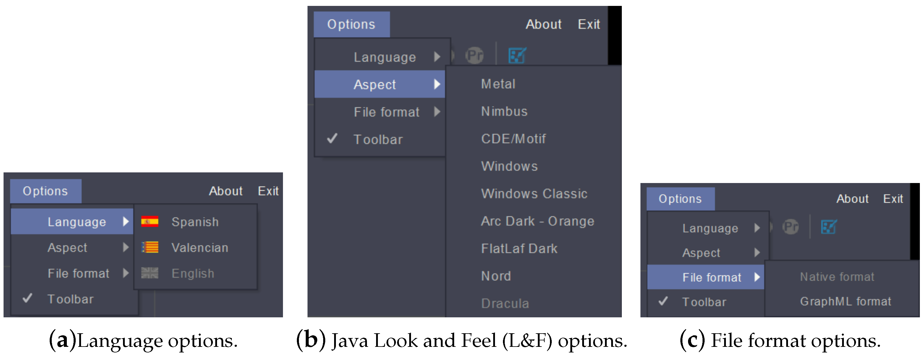
| An options item has been added to the main menu that includes the language selection, the Java L&F, the file format for graphs and a check box to set the visibility of the toolbar. |
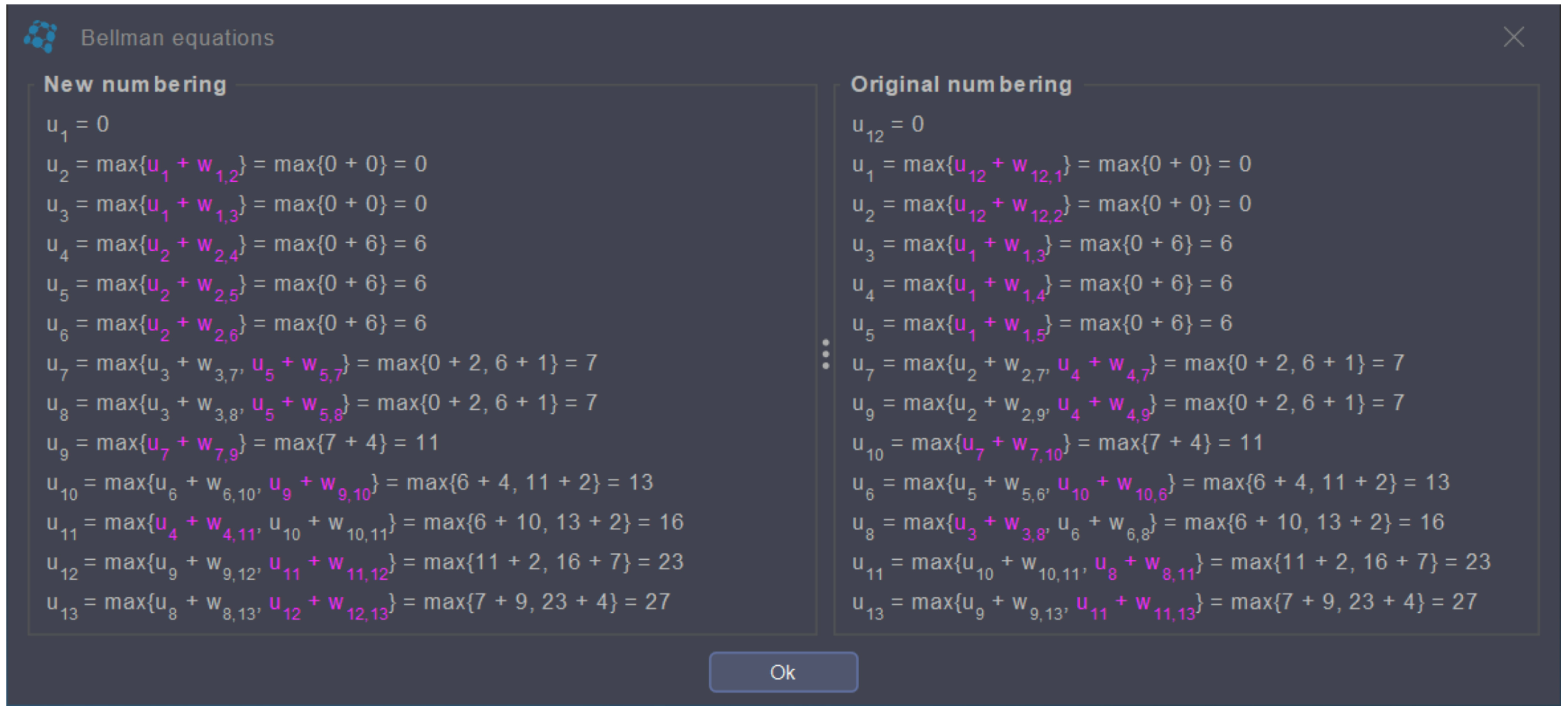
| For both the shortest path algorithm for acyclic graphs and the PERT algorithm, the explicit development of the Bellman equations is now displayed step by step, highlighting the value at which the minimum or maximum is reached, respectively, which is then used to identify the paths. |
| In the PERT algorithm, the maximum delay that can take place in completing a non-critical activity without affecting the project end date is now calculated. |
| For both the Dijkstra and Prim algorithms, the explicit development of each algorithm is also displayed step by step, mirroring the natural progression of the calculation process. |
| Item | Gender | Mode | Median | Lower Quartile | Upper Quartile |
|---|---|---|---|---|---|
| E1 | Female | 5 | 5 | 4 | 5 |
| Male | 4 | 4 | 4 | 4 | |
| Total | 4 | 4 | 4 | 4.75 | |
| E2 | Female | 5 | 5 | 4 | 5 |
| Male | 4 | 4 | 4 | 5 | |
| Total | 4 | 4 | 4 | 5 | |
| E3 | Female | 5 | 4 | 4 | 5 |
| Male | 4 | 4 | 3 | 4 | |
| Total | 4 | 4 | 3 | 4 | |
| E4 | Female | 5 | 5 | 4 | 5 |
| Male | 4 | 4 | 3 | 4 | |
| Total | 4 | 4 | 3 | 5 | |
| E5 | Female | 4 | 4 | 4 | 5 |
| Male | 4 | 4 | 3 | 4.75 | |
| Total | 4 | 4 | 3 | 5 | |
| C1 | Female | 4 | 4 | 4 | 5 |
| Male | 4 | 4 | 3 | 4 | |
| Total | 4 | 4 | 3 | 4 | |
| C2 | Female | 5 | 4 | 4 | 5 |
| Male | 4 | 4 | 4 | 4.75 | |
| Total | 4 | 4 | 4 | 5 | |
| C3 | Female | 4 | 4 | 4 | 5 |
| Male | 4 | 4 | 4 | 4 | |
| Total | 4 | 4 | 4 | 4 | |
| C4 | Female | 4 | 4 | 4 | 5 |
| Male | 4 | 4 | 4 | 5 | |
| Total | 4 | 4 | 4 | 5 |
| Item | Gender | Mode | Median | Lower Quartile | Upper Quartile |
|---|---|---|---|---|---|
| D1 | Female | 4 | 4 | 4 | 5 |
| Male | 4 | 4 | 3 | 5 | |
| Total | 4 | 4 | 3 | 5 | |
| D2 | Female | 4 | 4 | 4 | 5 |
| Male | 4 | 4 | 4 | 5 | |
| Total | 4 | 4 | 4 | 5 | |
| D3 | Female | 5 | 5 | 4 | 5 |
| Male | 5 | 4 | 3 | 5 | |
| Total | 5 | 4 | 4 | 5 | |
| D4 | Female | 4 | 4 | 4 | 5 |
| Male | 4 | 4 | 3 | 4 | |
| Total | 4 | 4 | 3 | 4.75 | |
| D5 | Female | 5 | 5 | 3 | 5 |
| Male | 5 | 4 | 4 | 5 | |
| Total | 5 | 4 | 4 | 5 | |
| D6 | Female | 5 | 4 | 3 | 5 |
| Male | 4 | 4 | 3 | 5 | |
| Total | 4 | 4 | 3 | 5 | |
| G1 | Female | 4 | 4 | 4 | 5 |
| Male | 4 | 4 | 4 | 5 | |
| Total | 4 | 4 | 4 | 5 | |
| G2 | Female | 4 | 4 | 4 | 5 |
| Male | 4 | 4 | 3 | 4 | |
| Total | 4 | 4 | 3 | 5 | |
| G3 | Female | 5 | 5 | 4 | 5 |
| Male | 4 | 4 | 4 | 4 | |
| Total | 4 | 4 | 4 | 5 |
| Model | Unstandardised Coefficients | Standardised Coefficients | |||
|---|---|---|---|---|---|
| Std. Error | Sig. | ||||
| Model A | Constant | −0.069 | 0.102 | 0.500 | |
| Female | 0.556 | 0.277 | 0.189 | 0.047 | |
| Model B | Constant | −0.160 | 0.098 | 0.108 | |
| Age [20–29] | 0.472 | 0.200 | 0.221 | 0.020 |
Disclaimer/Publisher’s Note: The statements, opinions and data contained in all publications are solely those of the individual author(s) and contributor(s) and not of MDPI and/or the editor(s). MDPI and/or the editor(s) disclaim responsibility for any injury to people or property resulting from any ideas, methods, instructions or products referred to in the content. |
© 2023 by the authors. Licensee MDPI, Basel, Switzerland. This article is an open access article distributed under the terms and conditions of the Creative Commons Attribution (CC BY) license (https://creativecommons.org/licenses/by/4.0/).
Share and Cite
Migallón, V.; Penadés, J. A Java Application for Teaching Graphs in Undergraduate Courses. Appl. Sci. 2023, 13, 12945. https://doi.org/10.3390/app132312945
Migallón V, Penadés J. A Java Application for Teaching Graphs in Undergraduate Courses. Applied Sciences. 2023; 13(23):12945. https://doi.org/10.3390/app132312945
Chicago/Turabian StyleMigallón, Violeta, and José Penadés. 2023. "A Java Application for Teaching Graphs in Undergraduate Courses" Applied Sciences 13, no. 23: 12945. https://doi.org/10.3390/app132312945
APA StyleMigallón, V., & Penadés, J. (2023). A Java Application for Teaching Graphs in Undergraduate Courses. Applied Sciences, 13(23), 12945. https://doi.org/10.3390/app132312945