A Strategy for Integrated Multi-Demands High-Performance Motion Planning Based on Nonlinear MPC

Abstract

Nonlinear Model Predictive Control (NMPC) is an effective approach for motion planning in autonomous vehicles that need to satisfy multiple driving demands. Within the realm of planner design, current strategies inadequately address the issues related to redundancy and conflicts among these diverse demands. This shortcoming leads to low efficiency and suboptimal performance, particularly when faced with a high volume of demands. In response to this challenge, this paper introduces the Hierarchical and Multi-Domain (HMD) strategy as a solution for designing a multi-objective NMPC planner. This strategy enables the dynamic adjustment of the integration method for demand indicators based on their priority. To evaluate the risk of breaching driving demands, several risk functions are established. The constraints and objective function of the planner are meticulously designed in accordance with the HMD strategy and evaluation functions. Simulation results attest to the advantages of the HMD-based planner, which, compared to planners based on traditional multi-objective (TMO) strategies, exhibits a 68.5% improvement in solution efficiency and the simultaneous enhancement of driving safety. Additionally, the HMD approach reduces the maximum jerk by 58.8%.

1. Introduction

In recent years, autonomous vehicles (AVs) have received significant attention due to their potential to satisfy various driving demands, such as collision avoidance and passenger comfort [1,2,3,4,5,6,7]. When addressing the complex challenge of integrated multi-demands, the prevailing approach involves formulating it as a multi-objective optimization problem [8,9]. In this context, the cutting-edge methodologies encompass Reinforcement Learning [10,11,12,13] and NMPC [14,15,16]. This paper specifically focuses on NMPC-based methods due to their clarity of mechanism. Ensuring the satisfaction of diverse driving demands while maintaining computational efficiency is a paramount concern.

When designing an NMPC planner under the TMO strategy, the process typically commences with the modeling of driving demands. Subsequently, fundamental demands, such as trajectory tracking, passenger comfort, and fuel economy, are aggregated in a weighted manner to construct the objective function. High-priority demands, including collision avoidance, dynamic stability, and adherence to traffic rules, are typically established as constraints [14,15,16,17,18,19,20,21,22]. For instance, references [15,16,17] developed an NMPC planner for emergency obstacle avoidance. They incorporated trajectory tracking errors into the objective function while imposing collision avoidance and dynamic stability models as constraints. Reference [8] integrated tracking error and control variables into the objective function, simultaneously applying speed limits and solid lane constraints. While these methods yielded favorable results, the TMO strategy encounters a challenge as the number of considered demands escalates. This results in a proliferation of constraints, leading to an exponential increase in the optimization dimension, subsequently diminishing computational efficiency [4].

This study encompasses the integration of prevalent driving demands, which include dynamic stability, collision avoidance, adherence to traffic rules (such as red light compliance, staying within solid lane lines, and observing maximum speed limits), fuel efficiency, passenger comfort, and tracking capability. While there is a dearth of research explicitly addressing all eight of these driving demands, it is evident that the TMO strategy is intrinsically unsuitable for this problem. In certain situations, such as when an AV is faced with the loss of dynamic stability, considerations such as driving comfort or fuel economy become secondary [18,22]. Combining the latter demands and the former incurs conflict and can potentially lead to collisions. Conversely, during simple tasks where dynamic stability is not a primary concern, AVs have no need to consider this aspect [14,21]. In such instances, the control of the vehicle operates well within the bounds of dynamic stability, rendering the dynamic stability constraint redundant. Eliminating this redundancy reduces the optimization dimension without compromising control performance.

To effectively address the issues of conflict and redundancy among driving demands (redundancy refers that the constraint corresponding to some demand is ineffective, i.e., removing the constraint does not affect the solution of optimization), this paper introduces HMD strategy to guide planner design. Initially, driving demands are systematically prioritized based on their impact on driving safety. Subsequently, leveraging these priorities, the HMD strategy assesses the potential risks of violating driving demands in a hierarchical sequence. To bolster safety, lower-priority demands that clash with higher-priority counterparts are either omitted or attenuated. Additionally, any demands that can be currently satisfied are removed. This process results in the segmentation of the demand domain into several sub-domains (see Figure 1). The motion planner focuses exclusively on the demands within one of these sub-domains. Several evaluation functions are established to gauge the risk of violating driving demands. The performance of the HMD-based planner is then compared to the TMO-based planner through simulations in typical scenarios.

The main contributions of this paper are:

1. This study proposes a scheduling strategy for driving demand indicators based on the characteristics of driving demands, such as the priority. This strategy enables the dynamic adjustment of the integration method for demand indicators, which can handle the conflict and redundancy among indicators well.

2. To determine whether driving demands are satisfied, several risk functions are established. Then, an integrated control model based on NMPC theory is designed. Typical scenarios in a simulation demonstrate that our controller improves comfort, fuel economy, and safety compared to a traditional controller.

The subsequent sections of this paper are organized as follows: Section 2 delineates the formulation of the NMPC planner under the TMO strategy. It subsequently elucidates the issues surrounding redundancy and conflicts through an analysis of three typical scenarios. In Section 3, the HMD strategy is elaborated upon, with the introduction of several functions designed to evaluate the potential breaches of driving demands. Subsequently, the constraints and the objective function are established based on these evaluation functions. Section 4 provides a comparative analysis of the results obtained using the HMD and TMO strategies. Finally, Section 5 draws the paper to a conclusion.

2. Problem Description

This section initiates the formulation of the NMPC planner under the TMO strategy. Subsequently, it delves into the issue of redundancy and conflict, providing an in-depth analysis through the examination of three typical scenarios.

The idea of TMO strategy is aggregating the fundamental demands into the objective function through a weighted manner, and transforming the high-priority demands function to the constraints directly. This strategy is commonly used in many papers [8,14,15,16,17]. The multi-objective NMPC planner under the TMO strategy is represented as follows:

$$\underset{\mathit{x},\mathit{u}}{\mathit{min}}\sum _{i=0}^{N_p-1}(q_1{f}_{track}^i+q_2{f}_{comf}^i+{q_{3}f}_{fuel}^i)$$

(1a)

$$\mathrm{s}.\mathrm{t}. \mathit{x}\left(0\right)={\mathit{x}}_0$$

(1b)

$${\mathit{x}}^{i+1}=\mathit{f}\left({\mathit{x}}^i,{\mathit{u}}^i\right), i=0\dots N_p-1$$

(1c)

$${\mathit{u}}_{min}\le {\mathit{u}}^i\le {\mathit{u}}_{max}, i=0\dots N_p-1$$

(1d)

$$C_{dyna}^i<0, i=0\dots N_p-1$$

(1e)

$$C_{colli}^i<0, i=0\dots N_p-1$$

(1f)

$$C_{lane}^i<0, i=0\dots N_p-1$$

(1g)

$$C_{red}^i<0, i=0\dots N_p-1$$

(1h)

$$C_{speed}^i<0, i=0\dots N_p-1$$

(1i)

where $N_p$ is the number of discretization points in prediction horizon. (1b) is the initial condition for vehicle state $\mathit{x}$. $\mathit{x}={\left[v_x v_y \omega s e_1 e_2\right]}^T$, in which $v_x, v_y$ are longitudinal and lateral speed, respectively. $\omega$ is the angular speed. $s,e_1,e_2$ are the position coordinates in Frenet coordinates [8]. $s$ denotes the longitudinal driving distance. $e_1,e_2$ are the lateral position and heading error with respect to the reference trajectory, respectively. (1a) is the objective function, in which $f_{track}^i, f_{comf}^i$ and $f_{fuel}^i$ describe the objectives of tracking, comfort, and fuel economy at $i$-th time step, respectively. $q_1, q_2 \mathrm{a}\mathrm{n}\mathrm{d} q_3$ are their weights. $f_{track}={(e_1-e_{1d})}^2+{e_2}^2+{(v_x-v_{xd})}^2,$ where $e_{1d}$ and $v_{xd}$ are the desired lateral position and longitudinal speed, respectively. $f_{comf}$ is the sum of the square of acceleration and jerk [14]. $f_{fuel}$ is the empirical formula of fuel consumption [21]. (1c) is the vehicle dynamics function [23]. (1d) is the physical control limits, and $\mathit{u}$ is the control input, including the driving force and steering angle of the front wheel. (1e)–(1i) describe the constraints of dynamic stability, collision avoidance, solid lane line, red light, and max speed limit, respectively. The specific models of these constraints are referred to [20].

To elucidate and analyze the issue of redundancy and conflict among driving demands, three typical scenarios are established, as illustrated in Figure 2. The initial states are depicted in the figure, with the red light 10 s remaining, and a maximum speed limit of 60 km/h. In the first two scenarios, the obstacle vehicles (OVs) are engaged in lane-keeping maneuvers at a constant speed. In the third scenario, OV1 abruptly changes lanes, decelerating to merge into the middle lane.

In planner (1), the TMO strategy mandates collision avoidance and adherence to solid lane lines as constraints for all scenarios. However, these constraints may prove ineffective in certain situations. In the scenario depicted in Figure 2a, the solid lane line is positioned within the side lanes, while the tracking demand necessitates that the subject vehicle (SV) travels along the centerline of the middle lane. If the tracking performance is optimal, the constraint related to the solid lane line becomes redundant. Additionally, all OVs are operating within their respective lanes, rendering collision avoidance constraints unnecessary. Similarly, constraints pertaining to dynamic stability and speed limits become redundant.

Conversely, in the scenario illustrated in Figure 2c, OV1 abruptly changes lanes and decelerates, necessitating a rapid reaction from the SV to avert a collision. To ensure safety, planner (1) should not consider factors such as comfort or fuel economy, as they could compromise the execution of swift control inputs, thereby conflicting with the imperative of collision avoidance. Furthermore, the constraint concerning adherence to solid lane lines contradicts the necessity for collision avoidance, potentially leading to collision incidents.

The removal of ineffective and conflicting constraints from the planner can enhance solving efficiency and driving safety. Nevertheless, the determination of whether driving demands are redundant or in conflict hinges upon the specific conditions of the vehicle’s operation. For example, in the scenario depicted in Figure 2b, both collision avoidance and adherence to solid lane lines remain non-redundant and non-conflicting.

To more effectively address the issues of redundancy and conflict among driving demands, the following section introduces the HMD strategy, which is founded on driving demands and serves as the basis for designing the NMPC planner.

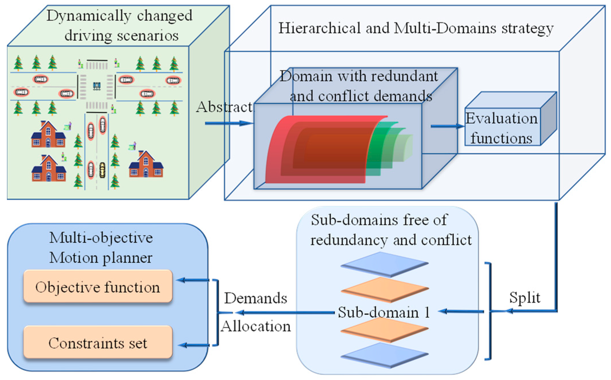
3. Hierarchical and Multi-Domains Strategy Based on Driving Demands

In this section, we introduce the HMD strategy as a means to formulate the constraints and objective function of the NMPC planner. Furthermore, we establish a set of risk functions, which are based on vehicle kinematics and tire dynamics. These functions are pivotal for evaluating whether there is a risk of breaching driving demands.

3.1. HMD Strategy

Before designing the scheduling strategy, the priority of driving demands needs to be determined first. Driving requirements can be categorized into safety, traffic rules, and entertainment classes (See Figure 3). Their priority classification is as follows.

Safety requirements take the highest priority, encompassing both dynamic stability and obstacle avoidance safety. The boundary of dynamic stability represents the working limits of the tires. If the vehicle control exceeds this boundary, it implies severe tire sliding, leading to a loss of control capabilities. As the loss of control compromises safety and other demands, the priority of dynamic stability is higher than obstacle avoidance safety.

Traffic rules include no crossing of road boundaries, no running red lights, and no speeding. Adhering to traffic rules is prioritized below safety demands and above entertainment demands. Running red lights or crossing a road boundary can easily lead to collisions; hence, they own the highest priority. Speeding owns the lowest priority.

Entertainment demands include tracking, fuel economy, and comfort. Tracking determines the direction and speed of vehicle, thus is the fundamental demand and holds the highest priority. Comfort, achieved by limiting acceleration and jerk, indirectly contributes to reduced energy, making comfort a higher priority than fuel economy.

As shown in Figure 4, the HMD strategy evaluates the driving demands according to the priority (See Figure 3). The HMD strategy initiates the evaluation process by first assessing safety-related demands; namely, dynamic stability. If the SV is at risk of losing dynamic stability, the HMD strategy temporarily sets aside considerations such as driving comfort, fuel economy, or adherence to traffic rules. Meanwhile, the collision avoidance demand is formulated as a penalization function instead of constraint, because conflict between two constraints may lead to the infeasibility of optimization. In cases where there is no risk to dynamic un-stability, the dynamic stability constraint is excluded from the NMPC planner so as to improve solution efficiency. When the SV faces a collision risk, the desired states for tracking demands are adjusted to avoid a collision. The specific process is described in Section 3.3. The comfort and fuel efficiency demands are kept in objective function to ensure the smooth changing of state trajectory.

When safety concerns are resolved, the HMD proceeds to evaluate demands related to traffic rules. No crossing of road boundaries and no running red lights share the same priority; thus, the HMD evaluates them concurrently (as depicted in Figure 4). If either of them may not be satisfied, the corresponding constraint will be added into the NMPC controller. Only when both of them can be guaranteed, the HMD will proceed to evaluate the no speed demand.

For the entertainment demands, they only exist in the objective function because of being the lowest priority. When there exist safety concerns, some of them could be removed to avoid conflict between demands. Among the three entertainment demands, their weights in objective function are determined based on their relative priority.

3.2. Evaluation Functions of Driving Demands

3.2.1. Dynamic Stability

The evaluation function of whether a vehicle has risks of losing dynamic stability is constructed based on the sideslip limit of tires. The final function is defined by Equation (6).

Beal et al. [22] established the vehicle dynamics stability boundary based on the sideslip limit of tires in the front axle and rear axle. The stability condition can be shown in the following form:

$$\left\{\begin{array}{c}{a}_y-\frac{F_{{yr}_{max}}(1+L_r/L_f)}{m}\le 0\\ a_y-\frac{F_{{yf}_{max}}(1+L_f/L_r)}{m}\le 0\end{array}\right.$$

(2)

where $a_y$ is the centroid lateral acceleration. $m$ is SV mass. $L_f, L_r$ are the distances from the centroid to the front and rear axles, respectively (See Figure 5).$F_{{yf}_{max}}, F_{{yr}_{max}}$ are the maximum lateral forces in the front and rear tires, respectively [22].

When the SV is accelerating, considering the weight transfer in the longitudinal direction of the vehicle, and the tire lateral–longitudinal force coupling, there are the following relations:

$$\left\{\begin{array}{c}{F}_{{yf}_{max}}=E(\sqrt{{(\frac{\mu m\left(-a_{x}z+g{L}_r\right)}{L})}^2-F^2})\\ F_{{yr}_{max}}=\frac{\mu Em\left(a_{x}z+g{L}_f\right)}{L}\end{array}\right.$$

(3)

where $F_{{yf}_{max}}, F_{{yr}_{max}}$, are the maximum front and rear axle lateral force, respectively. $F$ is driving force in front tire. $a_x$ is the longitudinal acceleration of the centroid. $z$ is the centroid height. $E$ is the ratio of the sliding friction coefficient to the peak coefficient. $g$ is gravity acceleration. $L$ is wheelbase. $\mu$ is the friction ground friction coefficient.

When SV is decelerating, suppose all the tires could lock at the same time. There is the following relation:

$$m{a}_{y_{max}}=E\sqrt{{\left(\mu mg\right)}^2-{\left(m{a}_x\right)}^2}$$

(4)

where $a_{y_{max}}$ is the maximum centroid lateral acceleration. Suppose $L_f<L_r$. Plug Equation (3) into (2) and combine Equation (4), we can obtain the stability condition in both the acceleration and deceleration situation:

$$\left\{\begin{array}{c}{(\frac{a_y}{\mu E})}^2-{\left(g-\frac{z{a}_x}{L_r}\right)}^2+{\left(\frac{a_{x}L}{\mu L_r}\right)}^2\le 0, a_x>0\\ {(\frac{a_y}{\mu E})}^2-g^2+{\left(\frac{a_x}{\mu }\right)}^2\le 0, a_x\le 0\end{array}\right.$$

(5)

Based on Equation (5) and the first-order Euler formula, the evaluation function of dynamic stability is defined as:

$$L_{dyna}=\left\{\begin{array}{c}{(\frac{a_y^{\prime }}{\mu E})}^2-{\left(g-\frac{z{a}_x^{\prime }}{L_r}\right)}^2+{\left(\frac{a_x^{\prime }L}{\mu L_r}\right)}^2, a_x>0\\ {(\frac{a_y^{\prime }}{\mu E})}^2-g^2+{\left(\frac{a_x^{\prime }}{\mu }\right)}^2, a_x\le 0\end{array}\right.$$

(6)

where $L_{dyna}$ is the evaluation function of whether the vehicle has risks of losing dynamic stability. $\left(a_x^{\prime },a_y^{\prime }\right)=\left(a_x+{\dot{a}}_x{T}_r,a_y+{\dot{a}}_y{T}_r\right)$, in which ${\dot{a}}_x,{\dot{a}}_y$ are the longitudinal and lateral jerk, respectively. $T_r$ is a time constant.

3.2.2. Collision Avoidance

To ensure the interpretability, the collision risky area is evaluated by the risky ellipse area of OV (See Figure 6). The correspondent evaluation function is defined as:

$$L_{colli}=1-{\left|\right|\mathit{R}{\mathit{X}}_{\mathit{r}}\left|\right|}_F^2$$

(7)

$$\begin{array}{c}\mathit{R}=\left[\begin{array}{ccc}cos\left({\theta }_i\right)& -sin\left({\theta }_i\right)& 0\\ 0& 0& sin\left({\theta }_i\right)\end{array} \begin{array}{c}0\\ cos\left({\theta }_i\right)\end{array}\right]\\ {\mathit{X}}_{\mathit{r}}={\left[\begin{array}{c}\frac{X-X_i}{l_a}\\ 0\end{array} \begin{array}{c}\frac{Y-Y_i}{l_a}\\ 0\end{array} \begin{array}{c}0\\ \frac{X-X_i}{l_b}\end{array} \begin{array}{c}0\\ \frac{Y-Y_i}{l_b}\end{array}\right]}^T\end{array}$$

where ${\left|\right|\ast \left|\right|}_F$ is the frobenius norm operator. $L_{dyna}$ is the evaluation function of whether the vehicle has risks of collision. $\left(X,Y\right), \left(X_i,Y_i\right)$ are the global cartesian coordinates of the SV centroid and i-th OV centroid, respectively. ${\theta }_i$ is the yaw angle error between the OV and SV. ${[l_a,l_b]}^T=\mathit{F}+\mathit{P}\mathit{V}$, in which $\mathit{F},\mathit{P},\mathit{V}$ are:

$$\mathit{P}=\left[\begin{array}{ccc}\mathrm{c}\mathrm{o}\mathrm{s}\left({\theta }_i\right)& \mathrm{s}\mathrm{i}\mathrm{n}\left({\theta }_i\right)& \mathrm{c}\mathrm{o}\mathrm{s}\left({\theta }_i\right)\\ -\mathrm{s}\mathrm{i}\mathrm{n}\left({\theta }_i\right)& \mathrm{c}\mathrm{o}\mathrm{s}\left({\theta }_i\right)& -\mathrm{s}\mathrm{i}\mathrm{n}\left({\theta }_i\right)\end{array}\begin{array}{c}\mathrm{s}\mathrm{i}\mathrm{n}\left({\theta }_i\right)\\ \mathrm{c}\mathrm{o}\mathrm{s}\left({\theta }_i\right)\end{array}\right]$$

$$\mathit{F}=[\begin{array}{cc}\frac{\sqrt{2}}{2}{L}_i& \frac{\sqrt{2}}{2}{W}_i\end{array}{]}^T,\mathit{V}=[\begin{array}{cccc}(v_x-v_{xi})T_r& (v_y-v_{yi})T_r& \frac{(a_x-a_{xi})T_r^2}{2}& \frac{(a_y-a_{yi})T_r^2}{2}\end{array}{]}^T$$

where $L_i,W_i$ are the length and width of i-th OV, respectively. $v_{xi},v_{yi}$ are the longitudinal and lateral speed of i-th OV in the vehicle coordinate of SV. The directions are shown in Figure 6. $a_{xi},a_{yi}$ are the longitudinal and lateral acceleration of i-th OV in the vehicle coordinate of SV. $T_r$ is a time constant.

3.2.3. Traffic Rules

The evaluation function of whether a vehicle has risks of violating a solid lane line, red light, and max speed limit are defined by Equations (8)–(10), respectively:

$$L_{lane}=v{T}_r+\frac{1}{2}a{T}_r^2-DLC$$

(8)

$$L_{red}=v{T}_{red}+\frac{1}{2}a{T}_{red}^2-D$$

(9)

$$L_{speed}=v+a{T}_r-v_{max}$$

(10)

where $L_{lane},L_{red},L_{speed}$ are, respectively, evaluation functions of whether the vehicle has risks of violating solid lane line, red light, and max speed limit. $v,a$ are the speed and acceleration of the SV centroid, respectively. $DLC$ is the distance from the centroid to the solid lane line along the direction of $v$ [24]. $D$ is the distance from the centroid to a red light along the direction of lane. $v_{max}$ is the max speed limit. $T_{red}$ is the left time of the red light.$T_r$ is a time constant. The value of $T_r$ is adjusted by experience. Given that time horizon is 2 s, $T_r$ is recommended to be in the vicinity of 2 s.

3.3. Design of Constraints Set and Objective Function

To make the planner adaptively remove the ineffective constraints and adjust the conflict items, several risk indicators are defined:

$$\begin{array}{c}{I}_d=\left\{\begin{array}{c}0, L_{dyna}\le 0\\ 1, L_{dyna}>0\end{array}\right., I_c=\left\{\begin{array}{c}0, L_{colli}\le 0\\ 1, L_{colli}>0\end{array}\right.\\ I_l=\left\{\begin{array}{c}0, L_{lane}\le 0\\ 1, L_{lane}>0\end{array}\right., I_r=\left\{\begin{array}{c}0, L_{red}\le 0\\ 1, L_{red}>0\end{array}\right., I_s=\left\{\begin{array}{c}0, L_{speed}\le 0\\ 1, L_{speed}>0\end{array}\right.\end{array}$$

(11)

where $I_d, I_c, I_l, I_r, I_s$ are parameters indicating whether the driving demands are satisfied. They indicate the dynamic stability, collision avoidance, solid lane line, red light, and max speed limit, respectively. The values of those parameters equal to 1 means having risks of violating the demands. The constraints set of the driving demands are designed as:

$$\mathit{I}\times \mathit{C}\le 0$$

(12)

where $\mathit{I}=\mathrm{d}\mathrm{i}\mathrm{a}\mathrm{g} (I_d,\left(1-I_d\right)I_c,\left(1-I_d\right)\left(1-I_c\right)I_l, \left(1-I_d\right)\left(1-I_c\right)I_r,\left(1-I_l\right)\left(1-I_d\right)\left(1-I_c\right)I_s)$. $\mathit{C}={\left[\begin{array}{ccccc}{C}_{dyna},& C_{colli},& C_{lane},& C_{red},& C_{speed}\end{array}\right]}^T$. $\mathit{C}$ is the demand function vector. $\mathit{I}$ is used to activate or deactivate some constraint. To avoid conflict between constraints (such as collision avoidance and lane boundary), instead of activating all constraints simultaneously, we choose to activate part of these constraints according to the working conditions. This can be achieved by defining the constraints as $\mathit{I}\times \mathit{C}<0$.

The objective function is designed as:

$$q_1{f}_{track}+q_4\left(1-I_d\right)\left(q_2{f}_{comf}+q_3{f}_{fuel}\right)+q_5{I}_d{I}_c{C}_{colli}$$

(13)

where $q_1~q_5$ are weights of different items. The definitions of the items in Equation (13) are consistent with those in Equations (1) and (11). When the SV is at risk of collision, the desired states for the tracking demand undergo modification. Initially, the HMD strategy assesses whether the detection points are situated within areas deemed to be at risk of collision (as illustrated in Figure 7). If all detection points fall within these collision-prone areas, the desired lateral position remains unaltered. However, the desired speed is adjusted to match that of the OV. Conversely, if any detection point is outside the risky area, the desired lateral position is realigned to the centerline of the lane corresponding to the detection point’s location, as depicted in Figure 7.

It is important to emphasize that when the side lane and the current lane of the SV are separated by a solid lane line (as depicted in Figure 7), the side lane is not considered under typical circumstances. The side lane is only taken into account in emergent situations, which are defined as instances where the SV faces the risk of collision and loss of stability. In such cases, if there are two detection points meeting the criteria, the HMD strategy gives priority to the one located in the left lane adjacent to the SV.

4. Simulation Validation and Analysis

This section commences by presenting the formulation of the NMPC planner under the HMD strategy. Subsequently, it proceeds to compare the performance of the HMD-based planner with the TMO-based planner. Lane keeping, overtaking, and emergency obstacle avoidance are the three mostly commonly seen scenarios for autonomous vehicles. To reveal the problems of the current method and the advantages of our method, it is suitable to choose the most commonly seen scenarios to design validation experiment.

4.1. Planner Formulation

The multi-objective planner based on the HMD strategy is formulated below:

$$\underset{\mathit{x},\mathit{u}}{\mathit{min}}\sum _{i=0}^{N_p-1}(q_1{f}_{track}^i+q_5{I}_d{I}_c{C}_{colli}+q_4\left(1-I_d\right)\left(q_2{f}_{comf}^i+q_3{f}_{fuel}^i\right))$$

(14a)

$$\mathrm{s}.\mathrm{t}. \mathit{x}\left(0\right)={\mathit{x}}_0$$

(14b)

$${\mathit{x}}^{i+1}=\mathit{f}\left({\mathit{x}}^i,{\mathit{u}}^i\right), i=0\dots N_p-1$$

(14c)

$${\mathit{u}}_{min}\le {\mathit{u}}^i\le {\mathit{u}}_{max}, i=0\dots N_p-1$$

(14d)

$$\mathit{I}\times {\mathit{C}}^{\mathit{i}}\le 0, i=0\dots N_p-1$$

(14e)

where (14a) defines the objective function as determined by (13). (14e) outlines the constraints associated with the driving demands. (14b) through (14d), respectively, correspond to the initial condition, the vehicle dynamics function, and the physical control limits.

The decision and control algorithm are executed within a simulation platform comprised of CarSim, PreScan, and Matlab/Simulink, while the optimization problem is resolved using CasADi [25,26]. The computational setup involves a workstation featuring an Intel Core i5-8250U processor (1.6 GHz) and 8 GB of RAM. The simulation project is conducted with a 0.05 s cycle. The prediction horizon spans 2 s, with additional parameters for planners and evaluation functions detailed in

Table 1. Parameters of planners.

Parameter	Value	Parameter	Value
$N_p$	20	${\mathit{u}}_{min}$	$[\begin{array}{c}-8000 N\\ -30 deg\end{array}]$
$q_1$	5	${\mathit{u}}_{max}$	$[\begin{array}{c}4000 N\\ 30 deg\end{array}]$
$q_2$	4	$q_4$	1
$q_3$	3	$q_5$	100
$\mu$	0.8	E	0.7422

and

Table 2. Parameters of evaluation functions.

Parameter	Symbols of Evaluation Functions
	${\mathit{L}}_{\mathit{d}\mathit{y}\mathit{n}\mathit{a}}$	${\mathit{L}}_{\mathit{c}\mathit{o}\mathit{l}\mathit{l}\mathit{i}}$	${\mathit{L}}_{\mathit{l}\mathit{a}\mathit{n}\mathit{e}}$	${\mathit{L}}_{\mathit{s}\mathit{p}\mathit{e}\mathit{e}\mathit{d}}$
$T_r$(s)	1	4	3	3

.

4.2. Scenario 1

The specific configuration of this scenario is depicted in Figure 2a. Figure 8 illustrates the trajectories of various vehicles. Notably, due to the overlap between the HMD-based and TMO-based trajectories, Figure 8 only presents outcomes of the HMD-based planner.

The maximum speed error between the HMD- and TMO-based algorithms is merely 0.8% (See Figure 9a,b). Consequently, the HMD-based planner demonstrates a performance level on par with the TMO-based planner in terms of fulfilling driving demands. In this specific scenario, only the constraint related to the red light is deemed effective. The HMD activates the red light constraint before the 10 s mark and subsequently removes all constraints related to driving demands after this point (as demonstrated in Figure 10). As a result of eliminating ineffective constraints, the HMD-based algorithm operates at a remarkable 74.5% faster pace than the TMO-based algorithm (as evidenced in Figure 9d).

4.3. Scenario 2

The concrete setting of this scenario is shown in Figure 2b. Figure 11 shows the trajectories of different vehicles.

Figure 11 shows that the TMO makes the SV closer to OV1 than the HMD. The reason is that the desired position of the TMO is the centerline of the middle lane all the time, while OV1 forces the SV to leave the middle lane. The compromised result is that the SV avoids OV1 as close as possible. That is bad because the SV would violate the boundary of collision avoidance constraint due to a control error (See Figure 12d, the boundary is defined by $C_{colli}=0$ in (1f)). Then, the SV needs to change the current control input quickly, which results in a higher vibration amplitude and frequency of acceleration and jerk (See Figure 12a–c). The maximum jerk of the HMD is 58.8% lower than that of the TMO. Through the trajectory in Figure 11 and acceleration in Figure 12a,b, it can be found that the HMD has satisfied other demands, i.e., solid lane line, dynamic stability, etc.

Figure 13a shows that the total fuel consumption of the HMD is almost the same as that of the TMO. The fuel consumption is computed by an empirical function [18]. However, the solving efficiency of the HMD-based algorithm is 68.5% higher than the TMO-based algorithm (See Figure 13b). During 3 s~4 s, both $I_l$ and $I_{c1}$ equal 1 (See Figure 13c), so although there is a risk of violating the solid lane line rule, its constraint does not appear in the planner (14). However, the SV does not cross the solid lane line (See Figure 11), because satisfying the tracking demand indirectly satisfies the solid lane line demand.

4.4. Scenario 3

The setting of the scenario is shown in Figure 2c. The SV drives with 15 m/s while the speed of the obstacle vehicle is shown in Figure 14. Figure 15 shows the trajectories of different vehicles.

Figure 15 and Figure 16c vividly illustrate that the SV following the TMO strategy collides with OV1 at approximately t = 2.5 s. In contrast, the SV operating under the HMD approach successfully executes emergent obstacle avoidance. Additionally, Figure 16a,b show that the HMD-based SV reacts more swiftly than its TMO-based counterpart. The reason behind this enhanced performance is attributed to the evaluation results of the risks of collision and loss of dynamic stability. These results become 1 when OV1 abruptly merges into the middle lane (as evident in Figure 17). Subsequently, the HMD-based SV promptly adjusts its desired position to the centerline of the right lane, temporarily prioritizing safety over comfort, fuel economy, and traffic rules. On the other hand, the TMO-based SV persists in tracking the centerline of the middle lane, striving for driving comfort and fuel economy. Moreover, the TMO retains the solid lane line constraint, which contributes to a delayed control input and constrained feasible regions, ultimately leading to the collision incident. During the implementation of the emergent obstacle avoidance task, the nonlinearity of the optimization problem escalates significantly. Consequently, the algorithm solving time substantially increases compared to normal situations (as observed in Figure 17d). The solving time of the TMO-based algorithm can exceed 5 s, indicating that its numerical stability is inferior to that of the HMD-based approach.

5. Conclusions

This paper introduces the HMD strategy to formulate a high-performance NMPC planner tailored for integrated motion planning that accommodates multiple driving demands. To evaluate the effectiveness of the HMD-based planner, several typical scenarios are devised and analyzed. Simulation results show that during the lane-keeping task, the HMD-based planner achieves a 74.5% boost in efficiency, with a minimal speed error of under 0.8% compared to the TMO. In the context of lane changing and overtaking tasks, the HMD enhances solving efficiency by 68.5%, while simultaneously enhancing driving safety. Moreover, it reduces the maximum jerk by 58.8% compared to the TMO. In a particularly challenging task involving emergent obstacle avoidance, the HMD successfully executes safe motion planning, whereas the TMO-based approach falls short.

In the future, we plan to incorporate the motion uncertainty of obstacles in the environment and the measurement uncertainty of vehicle states into consideration. We aim to investigate the design theory of integrated decision and control methods with a strong emphasis on stochasticity.

References

1. Liu, X.; Liu, X.; Liu, Z.; Shi, R.; Ma, X. A Solar-powered Bus Charging Infrastructure Location Problem under Charging Service Degradation. Transp. Res. Part D Transp. Environ. 2023, 119, 103770. [Google Scholar] [CrossRef]
2. Liu, X.; Qu, X.; Ma, X. Optimizing electric bus charging infrastructure considering power matching and seasonality. Transp. Res. Part D Transp. Environ. 2021, 100, 103057. [Google Scholar] [CrossRef]
3. Yan, H.; Ma, X.; Pu, Z. Learning Dynamic and Hierarchical Traffic Spatiotemporal Features with Transformer. IEEE Trans. Intell. Transp. Syst. 2022, 23, 2236–22399. [Google Scholar] [CrossRef]
4. Gao, F.; Han, Y.; Li, S.E.; Xu, S.; Dang, D. Accurate Pseudospectral Optimization of Nonlinear Model Predictive Control for High-performance Motion Planning. IEEE Trans. Intell. Veh. 2023, 8, 1034–1045. [Google Scholar] [CrossRef]
5. Guan, Y.; Ren, Y.; Sun, Q.; Li, S.E.; Ma, H.; Duan, J.; Cheng, B. Integrated Decision and Control: Toward Interpretable and Computationally Efficient Driving Intelligence. IEEE Trans. Cybern. 2023, 53, 859–873. [Google Scholar] [CrossRef] [PubMed]
6. Feng, G.; Dang, D.; He, Y. Robust Coordinated Control of Nonlinear Heterogeneous Platoon Interacted by Uncertain Topology. IEEE Trans. Intell. Transp. Syst. 2022, 23, 4982–4992. [Google Scholar] [CrossRef]
7. Wu, P.; Gao, F.; Li, K. Humanlike Decision and Motion Planning for Lane Change Based on Artificial Potential Field. IEEE Access 2022, 10, 4359–4373. [Google Scholar] [CrossRef]
8. Dang, D.; Gao, F.; Hu, Q. Motion Planning for Autonomous Vehicles Considering Longitudinal and Lateral Dynamics Coupling. Appl. Sci. 2020, 10, 3180. [Google Scholar] [CrossRef]
9. Zhu, M.; Wang, Y.; Pu, Z.; Hu, J.; Wang, X.; Ke, R. Safe, Efficient, and Comfortable Velocity Control Based on Reinforcement Learning for Autonomous Driving. Transp. Res. Part C Emerg. Technol. 2020, 117, 102662. [Google Scholar] [CrossRef]
10. Mynuddin, M.; Gao, W. Distributed Predictive Cruise Control Based on Reinforcement Learning and Validation on Microscopic Traffic Simulation. IET Intell. Transp. Syst. 2020, 14, 270–277. [Google Scholar] [CrossRef]
11. Lin, Y.; McPhee, J.; Azad, N.L. Anti-Jerk On-Ramp Merging Using Deep Reinforcement Learning. In Proceedings of the 2020 IEEE Intelligent Vehicles Symposium, Las Vegas, NV, USA, 19 October–13 November 2020. [Google Scholar] [CrossRef]
12. Xu, X.; Zuo, L.; Li, X.; Qian, L.; Ren, J.; Sun, Z. A Reinforcement Learning Approach to Autonomous Decision Making of Intelligent Vehicles on Highways. IEEE Trans. Syst. Man Cybern. Syst. 2020, 50, 3884–3897. [Google Scholar] [CrossRef]
13. Vamplew, P.; Dazeley, R.; Berry, A.; Issabekov, R.; Dekker, E. Empirical Evaluation Methods for Multiobjective Reinforcement Learning Algorithms. Mach. Learn. 2011, 84, 51–80. [Google Scholar] [CrossRef]
14. Li, S.; Li, K.; Rajamani, R.; Wang, J. Model Predictive Multi-Objective Vehicular Adaptive Cruise Control. IEEE Trans. Control Syst. Technol. 2011, 19, 556–566. [Google Scholar] [CrossRef]
15. Funke, J.; Brown, M.; Erlien, S.M.; Gerdes, J.C. Collision Avoidance and Stabilization for Autonomous Vehicles in Emergency Scenarios. IEEE Trans. Control Syst. Technol. 2017, 25, 1204–1216. [Google Scholar] [CrossRef]
16. Erlien, S.M.; Fujita, S.; Gerdes, J.C. Shared Steering Control Using Safe Envelopes for Obstacle Avoidance and Vehicle Stability. IEEE Trans. Intell. Transp. Syst. 2016, 17, 441–451. [Google Scholar] [CrossRef]
17. Brown, M.; Funke, J.; Erlien, S.; Gerdes, J.C. Safe Driving Envelopes for Path Tracking in Autonomous Vehicles. Control Eng. Pract. 2017, 61, 307–316. [Google Scholar] [CrossRef]
18. Wang, H.; Huang, Y.; Khajepour, A.; Zhang, Y.; Rasekhipour, Y.; Cao, D. Crash Mitigation in Motion Planning for Autonomous Vehicles. IEEE Trans. Intell. Transp. Syst. 2019, 20, 3313–3323. [Google Scholar] [CrossRef]
19. Dixit, S.; Montanaro, U.; Dianati, M.; Oxtoby, D.; Mizutani, T.; Mouzakitis, A. Fallah Trajectory Planning for Autonomous High-Speed Overtaking in Structured Environments Using Robust MPC. IEEE Trans. Intell. Transp. Syst. 2020, 21, 2310–2323. [Google Scholar] [CrossRef]
20. Weiskircher, T.; Wang, Q.; Ayalew, B. Predictive Guidance and Control Framework for (Semi-)Autonomous Vehicles in Public Traffic. IEEE Trans. Control Syst. Technol. 2017, 25, 2034–2046. [Google Scholar] [CrossRef]
21. Kamal, M.A.S.; Mukai, M.; Murata, J.; Kawabe, T. On Board Eco-Driving System for Varying Road-Traffic Environments Using Model Predictive Control. In Proceedings of the 2010 IEEE International Conference on Control Applications, Yokohama, Japan, 8–10 September 2010. [Google Scholar]
22. Beal, C.E.; Gerdes, J.C. Model Predictive Control for Vehicle Stabilization at the Limits of Handling. IEEE Trans. Control Syst. Technol. 2013, 21, 1258–1269. [Google Scholar] [CrossRef]
23. Gao, F.; Hu, Q.; Ma, J.; Han, X. A Simplified Vehicle Dynamics Model for Motion Planner Designed by Nonlinear Model Predictive Control. Appl. Sci. 2021, 11, 9887. [Google Scholar] [CrossRef]
24. Mammar, S.; Glaser, S.; Netto, M. Time to Line Crossing for Lane Departure Avoidance: A Theoretical Study and An Experimental Setting. IEEE Trans. Intell. Transp. Syst. 2006, 7, 226–241. [Google Scholar] [CrossRef]
25. Duan, J.; Gao, F.; He, Y. Test Scenario Generation and Optimization Technology for Intelligent Driving Systems. IEEE Intell. Transp. Syst. Mag. 2022, 14, 115–127. [Google Scholar] [CrossRef]
26. Gao, F.; Han, Z.; Zhou, J.; Yang, Y. Performance Limit Evaluation by Evolution Test with Application to Automatic Parking System. IEEE Trans. Intell. Veh. 2023, 8, 3096–3105. [Google Scholar] [CrossRef]
Figure 1. The pipeline of decision and planning based on the HMD strategy.
Applsci 13 12443 g001
Figure 2. Scenarios with integrated driving demands. (a) Lane keeping before the red light intersection. (b) Consecutive overtaking before the red light intersection. (c) Emergent obstacle avoidance.
Applsci 13 12443 g002
Figure 3. Priority of driving demands.
Applsci 13 12443 g003
Figure 4. Hierarchical and multi-domains strategy.
Applsci 13 12443 g004
Figure 5. Schematic of forces in dynamic bicycle model.
Applsci 13 12443 g005
Figure 6. Illustration of variables in evaluation function of collision avoidance.
Applsci 13 12443 g006
Figure 7. Situation where SV faces risk of collision and would turn left.
Applsci 13 12443 g007
Figure 8. Trajectories of different vehicles based on HMD strategy.
Applsci 13 12443 g008
Figure 9. Speed trajectories and solving time of HMD and TMO. (a) Longitudinal speed. (b) Lateral speed. (c) Yaw rate. (d) Solving time.
Applsci 13 12443 g009
Figure 10. Evaluation results of different evaluation functions in scenario 1.
Applsci 13 12443 g010
Figure 11. Trajectories of different vehicles based on HMD strategy and TMO in scenario 2.
Applsci 13 12443 g011
Figure 12. Acceleration, jerk and collision risk of HMD and TMO. (a) Longitudinal acceleration. (b) Lateral acceleration. (c) Jerk. (d) Collision risk.
Applsci 13 12443 g012
Figure 13. Fuel consumption and solving time of HMD and TMO. Evaluation results of different evaluation functions. (a) Accumulated fuel consumption. (b) Lateral acceleration. (c) Evaluation results.
Applsci 13 12443 g013
Figure 14. Speed of obstacle vehicle. (a) Longitudinal speed. (b) Lateral speed.
Applsci 13 12443 g014
Figure 15. Trajectories of different vehicles based on HMD strategy and TMO in scenario 3.
Applsci 13 12443 g015
Figure 16. Acceleration, time to collision, and solving time of HMD and TMO. (a) Longitudinal acceleration. (b) Lateral acceleration. (c) Time to collision. (d) Solving time.
Applsci 13 12443 g016
Figure 17. Evaluation results of different evaluation functions in scenario 3.
Applsci 13 12443 g017